Method for fast determination of the angle of ionizing radiation incidence from data measured by a Timepix3 detector

This paper presents a method of how to determine spatial angles of ionizing radiation incidence quickly, using a Timepix3 detector. This work focuses on the dosimetric applications where detectors and measured quantities show significant angle dependencies. A determined angle of incidence can be used to correct for the angle dependence of a planar Timepix3 detector. Up until now, only passive dosemeters have been able to provide a correct dose and preserve the corresponding incidence angle of the radiation. Unfortunately, passive dosemeters cannot provide this information in “real” time. In our special setup we were able to retrieve the spatial angles with a runtime of less than 600 ms. Employing the new Timepix3 detector enables the use of effective data analysis where the direction of incident radiation is computed from a simple photon event map. In order to obtain this angle, we combine the information extracted from the map with known 3D geometry surrounding the detector. Moreover, we analyze the computation time behavior, conditions and optimizations of the developed spatial angle calculation algorithm.

1 Introduction

The national radiation protection regulations are all based on the European directive “council directive 2013/59/EURATOM” (European Parliament, 2013). This basic safety standard states the required dosimetry and the dose limits. Dosemeters are used to ensure that the prescribed dose limits for occupationally exposed workers are kept and to help reveal radiation protection issues in their environment. Therefore, these dosemeters must be able to measure the radiation dose accurately and provide a warning signal, preferably at the same time, if the radiation dose rate exceeds a predefined limit. A major difficulty for current active dosemeters that are based on semiconductors is that their planar geometry inherently has a non-uniform angular dependence on the photon detection efficiency, which directly affects their response. Knowledge of the true spatial angle of the incident radiation is necessary to allow for corrections of this dependence. Since the desired measurand is a body dose equivalent that relates the measured energy to the energy deposition at a certain depth in human tissue, the incident angle has an additional importance. Today, this information allowing proper transformation into the personal dose equivalent is only achieved using passive dosemeters. Not only can the information be used to optimize the accuracy of the dose rate measurement, it also supports radiation protection itself by indicating the direction of radioactive sources. In this paper we describe how we use a planar photon detector in the form of a silicon semiconductor bound on a hybrid pixel detector called Timepix3 (Poikela et al., 2014) to obtain information about the spatial angles of incident radiation. During measurements a thin aluminum foil shielded the photon detector with the aim of reducing interference from the low-energy photons of the ambient light. Our approach allows quick calculation of the direction of incident photons by using the known geometry of the direct surroundings of the detector. In our case, we use pins placed in front of the sensor and analyze the geometry of the pin's shadow as seen in the pixel matrix. Because the runtime of such an algorithm is heavily dependent on the allowed range for the radiation angle, the following evaluation is carried out respecting the German PTB requirements for stationary dosimetry PTB-A 23.3 (Physikalisch Technische Bundesanstalt, 2013b) regarding spatial angles.

1.1 Related work

There are many tried and tested techniques for obtaining spatial angles of incident radiation and to correct for any angular dependence that have been used for decades. For instance, one method that corrects the angle dependence of planar detectors is the glide-shadow effect (Ambrosi et al., 1994). This effect is used by passive dosemeters using an X-ray film as the planar detector. They are used for legal personal dosimetry in Germany and are collected after exposure by the relevant authority. The dominating radiation direction can be, but normally is not, retrieved from the shadows created by additional shielding pins on the film. Another example is the pinhole (Baek et al., 2013) and Compton camera (Sakai et al., 2019; Kormoll, 2013; Turecek et al., 2020). These, for example, are used during the demolition of nuclear power plants, for nuclear waste monitoring or in medical applications to trace back sources of gamma radiation. Since pinhole cameras require heavy shielding materials and Compton cameras rely on computationally demanding reconstruction algorithms, such approaches are not suitable for personal dosimetry. We use an approach that is based on the conditional density propagation (CONDENSATION) algorithm (Blake and Isard, 1997). This algorithm has been proven to be fast enough since it has already been used to track the spatial location of complex objects based on images. For instance, the algorithm can be used for the “real”-time application in context with robotics navigation (Roy et al., 2017). The algorithm we developed is derived from the CONDENSATION algorithm to calculate angles from the shadows located on the detector plane.

1.2 Timepix3

The Timepix3 chip was developed by the international Medipix3 collaboration of CERN (Medipix3 Collaboration, 2018). This chip has a 256×256 px array distributed over an area of 14 mm² with a pitch of ∼55 µm, which allows for pixel-wise time-resolved particle detection. It comes with a time resolution of 1.56 ns while offering a pixel rate of up to 40 MHits s⁻¹ cm⁻². In this instance the Timepix3 chip was used in conjunction with a 300 µm thick silicon semiconductor detector in order to catch high energetic photons. The data acquisition was done in data-driven mode, which returns a stream of pixels as they were hit (Poikela et al., 2014; Frojdh et al., 2015).

2 Methods

2.1 The Timepix3 measurement setup

The measurement setup, constructed in PTB, maintains the fixed pin positions even when used with different Timepix3 detectors. It consists of pins glued into a thin PMMA plate glued to an aluminum window which is in turn glued to an aluminum carrier plate located 2 mm above the sensor area of the Timepix3 chip. The carrier plate is exchangeable, allowing different pin materials, different window thicknesses and different pin configurations to be tested. In this case we used nine identical pins made of steel placed in a circular array. This configuration was chosen to obtain the best shadow-to-detector overlap while, at the same time, staying mostly independent of the rotation angle β. The angle β is defined as the rotation around the normal vector which stands perpendicular on the aluminum window and by that defines the z axis. In order to decrease the instability of the shadow detection, this pin configuration minimizes the relative shadow area that is not overlapping the detector. As only the gradient angle on the detector plane is important, our symmetrical setup does not obscure any relevant information. Moreover, the overall stability is improved by the 30 µm thick aluminum window whose purpose is to absorb low-energy photons from the ambient light and thereby reduce the background noise.

2.2 Input data

For the data acquisition, we used the data-driven mode of Timepix3, where all pixel information is transmitted once it has been hit. All pixel information consists of its coordinates, time of arrival and time over threshold. That gives us a maximum data rate of 440 MB s⁻¹ that is transformed into a series of frames as described in the following. The data fetched by a Timepix3 detector, using the previously described measuring setup, are integrated over a certain time depending on the actual count rate measured by the detector. In this case each ionizing event is observed regarding its location only. Neither the number of events per pixel nor the total duration that a pixel was active during the integration interval was taken into account. The resulting image only contains the information about which pixels were active. This procedure was chosen to keep the pre-processing to a minimum. Integrating these data over a certain time led to the following image in Fig. 2.

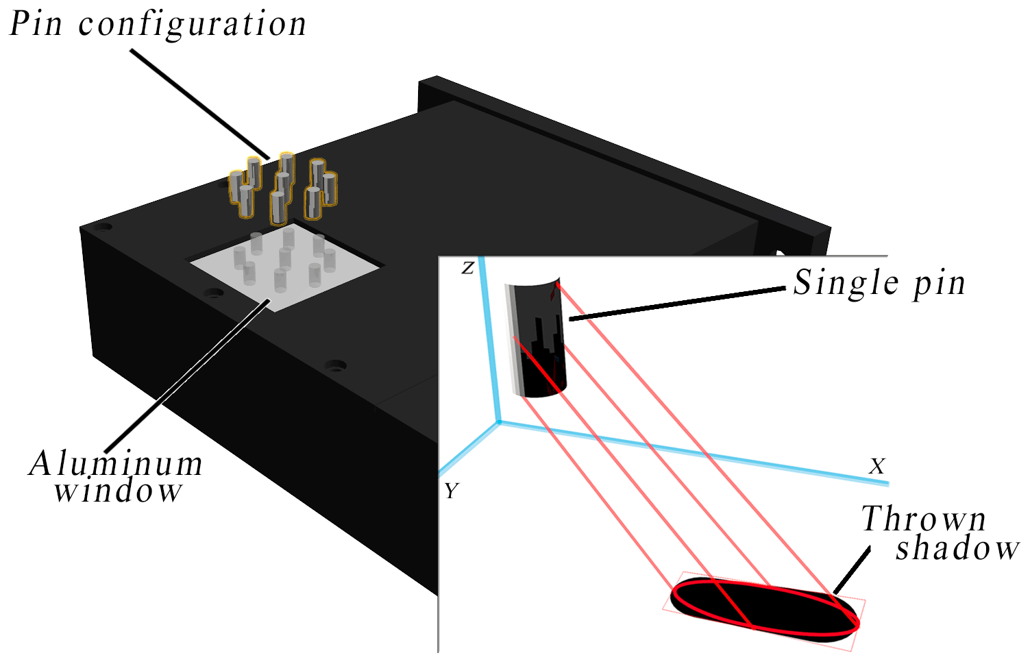
Figure 1 3D explosion drawing of the constructed dedicated Timepix3 measurement setup. It contains the configuration of the pins (highlighted in orange) as used. Shown in the lower right part of the diagram is a schematic shadow projection of one pin. This depiction shows the projection from the simplification of the geometry to the actual ellipse of the shadow particle.

Figure 2 Integrated Timepix3 data over a time of 10 ms using a radiation quality of H-60 (ISO, 2019) and under a gradient angle of 15^∘. A typical frame like this consists of roughly 12 000 photon events.

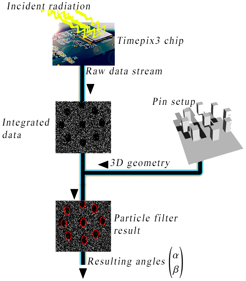
Figure 3 Snippet of the relevant parts of the schematic processing pipeline overview used to test the radiation angle detection algorithm.

2.3 Shadow and radiation angle detection algorithm

The flow diagram from Fig. 3 shows the different processing steps of the algorithm ending with the actual shadows and the resulting spatial angles. For testing purposes instead of a real device, previously recorded data from a file can also be used. The visual processing of the shadows is implemented using OpenCL (Munshi, 2012) and should be processed on a GPU for the best performance (datascience.com, 2018). The full source code is available under the MIT license (Lehner, 2019). The detection of shadows and their positions is done by processing the Timepix data collected over a fixed time interval or photon event count. We used 12 000 events to create one integrated frame. The schema of the data flow beginning at the integration up to the resulting radiation angle is shown in Fig. 3. The algorithm used is derived from the family of the “particle filters”, which itself is a subset of the Monte Carlo simulations. Our angle detection algorithm is adapted from the CONDENSATION algorithm (Blake and Isard, 1997). However, in contrast to that algorithm, our algorithm does not try to estimate the 2D positions of the individual shadows but estimates the 3D spatial angles of the radiation that created the shadows on the detector. This is achieved by using the known 3D geometry of the pin filters attached to the aluminium carrier plate above the detector and calculating the single particles based on that information. For reasons of efficiency complex pin geometries are simplified by a boundary box. The rectangular projected shadow will then be transformed into a fitting ellipse to leave out the noisy corners of a shadow. Note that particles in this context refer to instances of possible radiation directions whose probabilities can be computed from the given data at a time. As a consequence, the single particles $s_t^{\left(n\right)}$ are defined by the tuple ($\begin{array}{c}\mathit{\alpha }\\ \mathit{\beta }\end{array}$), where α describes the gradient angle, while β defines the rotation around the z axis. In the following a subscripted t will stand for a certain time, and a superscripted n indicates different instances of a particle given a time. Subsequently, a particle results in a complete possible shadow cast by all pins in the setup. Such a particle can then be validated against a measured frame. The algorithm uses that validation to iteratively maximize the probability of the hidden state represented by a particle. Since a particle represents the spatial direction relative to our detector, that maximization finds the best estimate for the real spatial direction. In order to smoothen the result, the weighted sum of all sufficiently possible particles is calculated to decrease the noise of the output:

$$\begin{array}{}\text{(1)}& {\displaystyle }& {\displaystyle }{S}_{t,\mathit{\gamma }}=\left\{s_t^{\left(n\right)}|R_{{\mathrm{s}}_{\mathrm{t}}^{\left(n\right)}}\ge \mathit{\gamma },n\le N\in \mathbb{N}\right\},\text{(2)}& {\displaystyle }& {\displaystyle }\mathit{\xi }\left[S_{t,\mathit{\gamma }}\right]=\sum _{n=\mathrm{1}}^M{\mathit{\pi }}_{\mathrm{w}}^{\left(n\right)}\cdot f\left(S_{t,{\mathit{\gamma }}_n}\right),M=\left|S_{t,\mathit{\gamma }}\right|,\end{array}$$

where

• ξ[S_t,γ] is a tuple ($\begin{array}{c}\mathit{\alpha }\\ \mathit{\beta }\end{array}$) that represents the final result of the shadow detection algorithm at time t.

• ${\mathit{\pi }}_{\mathrm{w}}^{\left(n\right)}$ is the weights of all items in S_t,γ. The condition $\sum _{n=\mathrm{1}}^M{\mathit{\pi }}_{\mathrm{w}}^{\left(n\right)}=\mathrm{1}$ must be fulfilled by all ${\mathit{\pi }}_{\mathrm{w}}^{\left(n\right)}$ in order to weight all values correctly.

• γ is a specific threshold depending on the mean noise. Possible values for it will be discussed alongside the results in Sect. 3.

• $R_{{\mathrm{s}}_t}^{\left(n\right)}$ is interpreted as the probability of a particle and is calculated by computing the quotient of shadowed pixels to existing pixels inside of the area defined by a particle $s_t^{\left(n\right)}$.

• S_t,γ. The set S_t,γ contains all the particles whose probability or hit-to-unhit pixel ratio is above the γ threshold that needs to be determined beforehand. The content of this set will be optimized during each iteration of the algorithm.

• $f\left(S_{t,{\mathit{\gamma }}_n}\right)$ is a mapping of a particle $S_{t,{\mathit{\gamma }}_n}$ into the set of possible angles of incidence ℝ².

• $|S_{t,\mathit{\gamma }}$ provides the count of items in the set S_t,γ.

The final result ξ[S_t,γ] will be computed from Shadows_t,γ containing the best result for the spatial radiation direction. Inside of ξ the mapping $f(s_t^{\left(n\right)}$ will map each particle $s_t^{\left(n\right)}$ onto its generation tuple ($\begin{array}{c}\mathit{\alpha }\\ \mathit{\beta }\end{array}$).

In order to transform a spatial angle tuple ($\begin{array}{c}\mathit{\alpha }\\ \mathit{\beta }\end{array}$) of a particle s_t to a “shadow ratio”. Ratio${}_{s_t}$, a simple parallel projection matrix P is used on every vertex v of the 3D geometry of the pins.

$$\begin{array}{}\text{(3)}& \begin{array}{rl}\mathbf{P}\mathit{v}& =\left(\begin{array}{ccc}\cos \left(\mathit{\beta }\right)& -\sin \left(\mathit{\beta }\right)& -\sin \left(\mathit{\beta }\right)\cdot \tan \left(\mathit{\alpha }\right)\\ \sin \left(\mathit{\beta }\right)& \cos \left(\mathit{\beta }\right)& \cos \left(\mathit{\beta }\right)\cdot \tan \left(\mathit{\alpha }\right)\\ \mathrm{0}& \mathrm{0}& \mathrm{0}\end{array}\right)\cdot \left(\begin{array}{c}x\\ y\\ z\end{array}\right)\\ & =\left(\begin{array}{c}x\cdot \cos \left(\mathit{\beta }\right)-(y+z\cdot \tan (\mathit{\alpha }\left)\right)\cdot \sin \left(\mathit{\beta }\right)\\ x\cdot \sin \left(\mathit{\beta }\right)+(y+z\cdot \tan (\mathit{\alpha }\left)\right)\cdot \cos \left(\mathit{\beta }\right)\\ \end{array}\right)\end{array}\end{array}$$

This results in a mapping of the pin geometry in the xy plane which will be interpreted as the detector area. The mapping is then used to compute the value of Ratio${}_{s_t^{\left(n\right)}}$ for any particle $s_t^{\left(n\right)}$ guessed by the algorithm. A scheme of this mapping for one single pin is portrayed in Fig. 1.

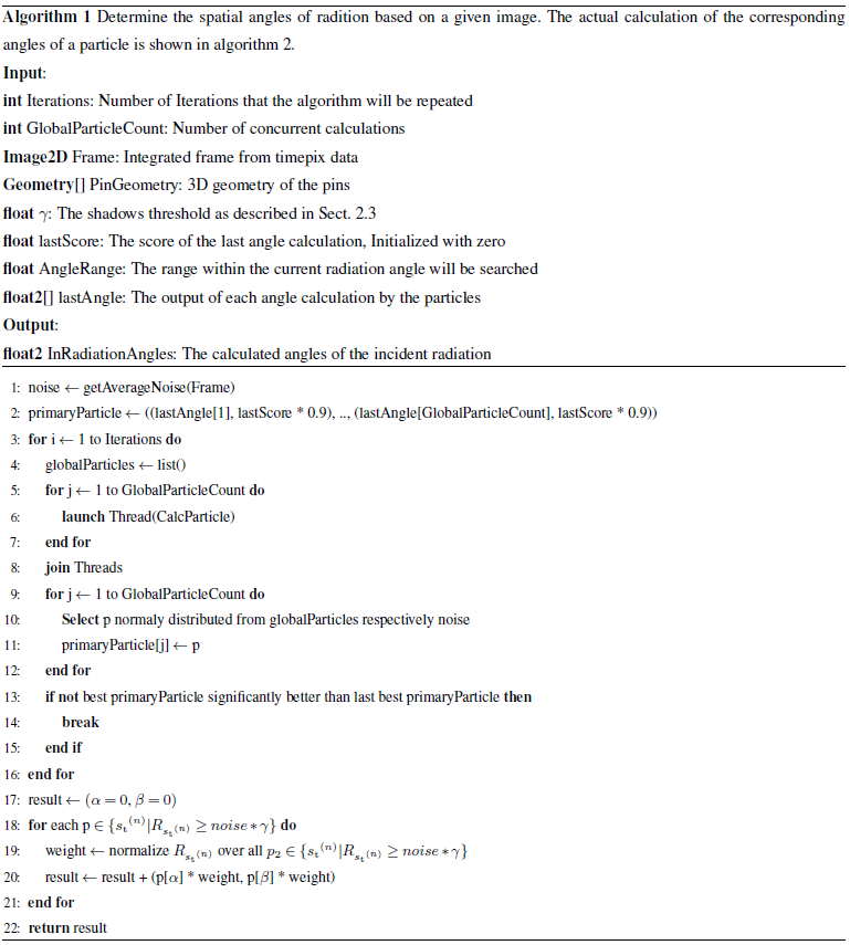
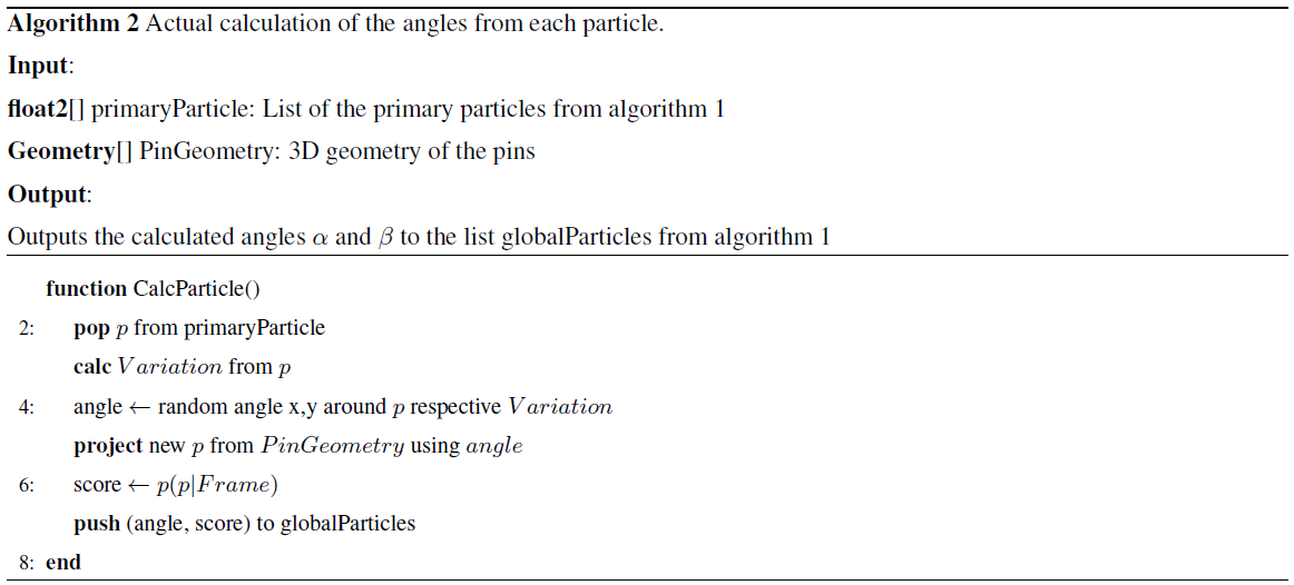
Hence the used particle filter algorithm works as shown in the following algorithm pseudo code (Algorithms 1 and 2).

3 Results

The algorithm for the incident radiation angle determination used here was tested by using the H-60 radiation quality (ISO, 2019) under gradient angles $\mathit{\alpha }\in [-\mathrm{45}$, $+\mathrm{45}{}^{\circ }]$ and 5^∘ steps. This is the angle range demanded by the PTB-Requirements for area dosemeters PTB-A 23.3 (Physikalisch Technische Bundesanstalt, 2013b).

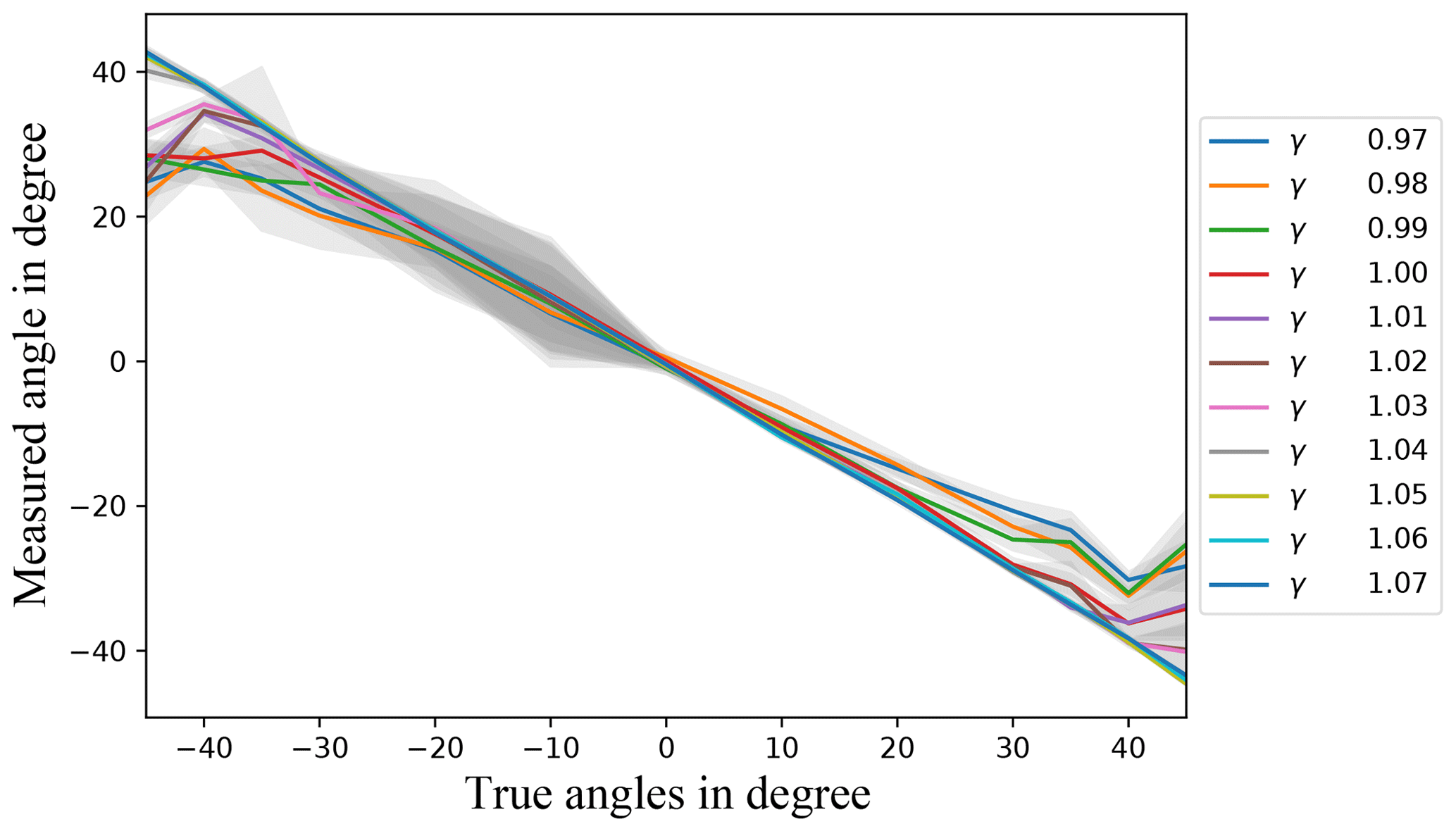
Figure 4 Radiation incident angles using data measured by the Timepix3 detector with the algorithm plotted over the true angles α. Each data point here was generated by calculating the mean value over five successive frames with the same true incident angle α and five evaluations of the same frame. The measurement was done using an H-60 radiation quality (ISO, 2019). The different lines correspond to one γ that was used as the shadow threshold in the shadow detection algorithm. The standard deviation is indicated by the grey backdrop area.

In this case, the measurement with a H-60 radiation quality corresponds to a dose rate of 173.2 mGy h⁻¹. Each test was repeated using a different γ∈[0.97, 1.07]. The value of γ was used as the shadow threshold in the shadow detection algorithm as described in Sect. 2.3. All following results from the algorithm were generated using a Windows 10 machine that was run with an Intel Xeon E5-1650 V3 CPU combined with a dedicated NVIDIA GTX 980 Ti GPU. Using this setup the runtimes of the algorithm with γ∈[0.97, 1.07] do not differ by more than 10 % from each other, so we used this interval to test the incident angle calculation. For all γ values used, the runtime for calculating the angles can be considered to be below 600 ms.

As can be seen in Fig. 4, most of the values used for γ result in values very close to the true angles. This figure was generated from test measurements using an H-60 radiation quality (ISO, 2019) with each data point being generated by calculating the mean value over five successive frames with the same true incident radiation angle α and five evaluations of the same frame. That means that we have tested the algorithm over a total time of 180 ms per γ value. Each measured angle in Fig. 4 corresponds to the mean value of 25 values per true angle. In addition, the gray underlay visualizes the standard deviation uniformly in the ±y direction. Interestingly the standard deviation is higher for negative α values. This is caused by an asymmetric pin configuration as a result of it being hand crafted. For all tested values of γ a good linear regression coefficient R² can be retrieved. Therefore, the results for some values of γ that are slightly rotated around the origin can be corrected depending on γ. This can be seen in Fig. 5. Furthermore, this figure shows the effect of γ reasonably well since higher values of γ result in a higher linear dependency, while lower values achieve a lower linear dependency.

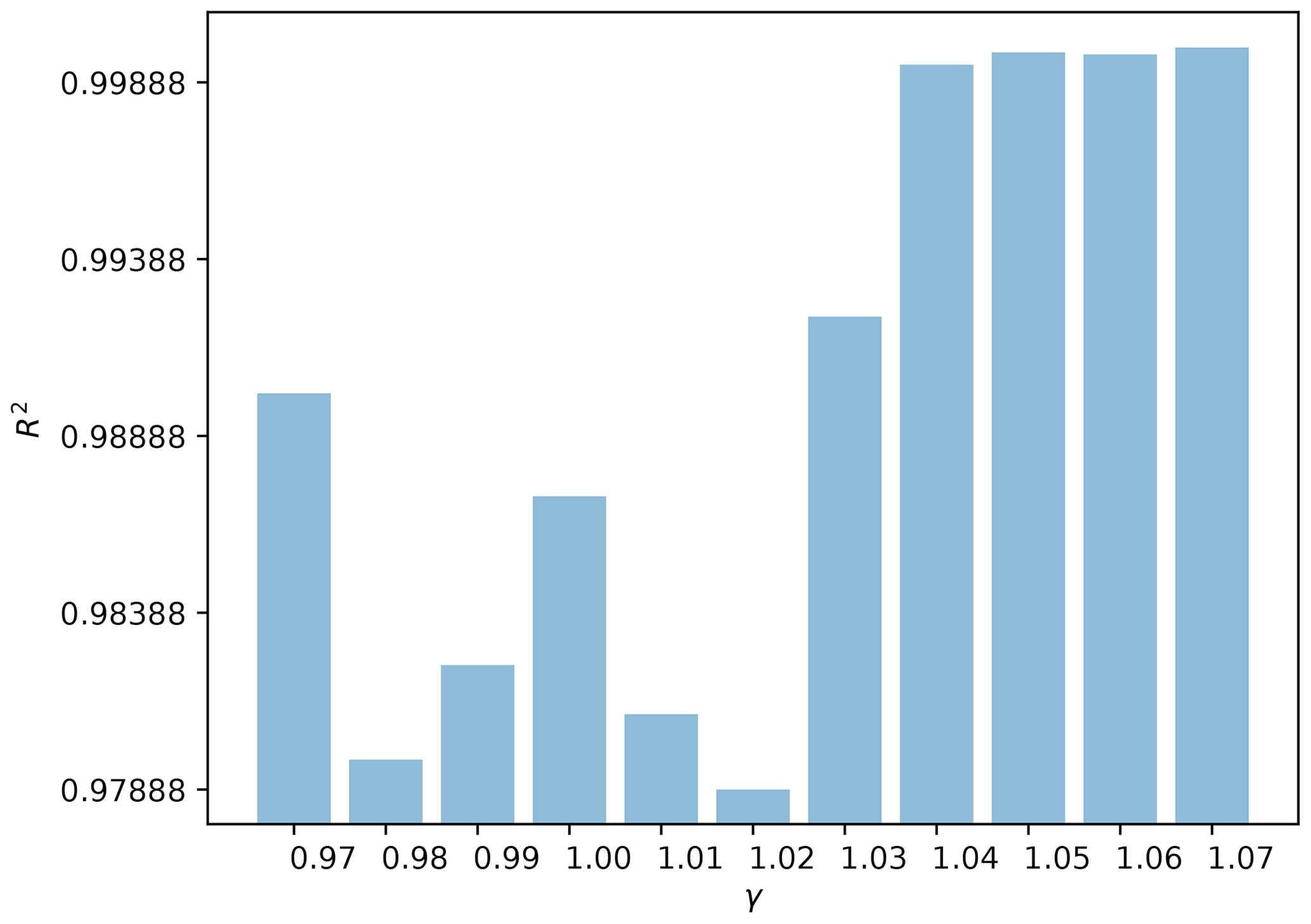
Figure 5 The linear regression coefficients R² for each γ used and the data points from Fig. 4.

It can be seen from Figs. 4 and 6 that all values for γ∈[0.97, 1.07] show a reasonable accuracy for $\mathit{\alpha }\in [-\mathrm{35}$, $+\mathrm{35}{}^{\circ }]$. Furthermore, Fig. 6 shows that there is a huge discrepancy between the single values of γ. That simply reflects the lower relative part of the pin configuration shadow that overlaps with the detector when the incident radiation angle increases. Hence the threshold γ needs to be higher in order to increase the probability of finding the shadow in the Timepix3 data since the algorithm's solution space is restricted by it. As can be seen using γ∈[1.03, 1.07], it still provides a reasonable accuracy for incident angles $\left|\mathit{\alpha }\right|\in (+\mathrm{35}$, $+\mathrm{45}{}^{\circ }]$.

Figure 6 The root mean square error (RMSE) over all gradient angles [−45, +45^∘] plotted over different values for γ. Each point corresponds to the measurements of five frames evaluated five times each.

The above observation validates the decision to consider γ as a variable in the algorithm, since an optimization of γ for the individual situation optimizes the algorithms' runtime too. The influence of γ gets stronger with the absolute angle of incidence. This is because higher values of γ not only increase the probability of a good result, but also could end with no result at all as well. That is represented in Fig. 7. There it can be seen that above an absolute incident radiation angle of 30^∘ the probability of no result with a γ after one complete evaluation rises quickly with the size of γ itself. However, it can be seen that a γ of 1.05 would after all still be a good choice in this case regarding the computation time and the accuracy.

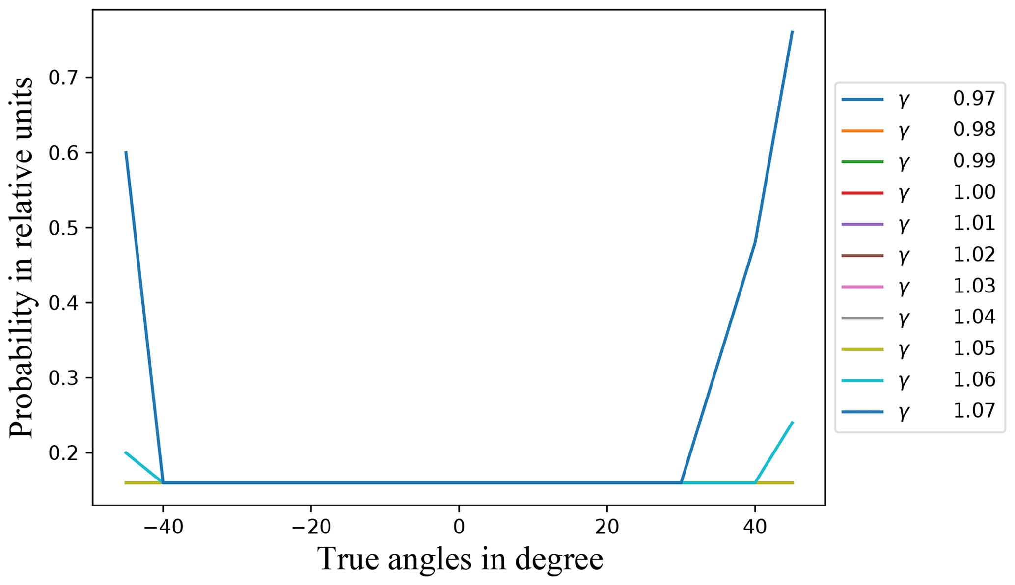
Figure 7 Probability of the algorithm producing no result after one complete execution for each value of γ.

The effectiveness of this approach is limited by the energy of the individual photons and the shielding capability of the pins, since a measurable contrast between light and shadow must exist. As soon as the pins shield too few photons, the angle detection becomes unstable or not feasible. In this case the algorithm does not return a result.

4 Conclusion

In this paper we presented a novel approach to the construction of solid-state dosemeters using an angle detection algorithm which converts the shadows on the detector into spatial angles and the pin construction above the detector surface, which serves as input for the algorithm.

As has been pointed out, the algorithm can approximate the spatial angle of incident radiation quite well if the algorithm is properly configured and used with incident radiation angles $\mathit{\alpha }\in [-\mathrm{45}$, $+\mathrm{45}{}^{\circ }]$ as required by PTB-A 23.3 (Physikalisch Technische Bundesanstalt, 2013b). While this is fully acceptable for use in area dosimetry in Germany (Physikalisch Technische Bundesanstalt, 2013b), it is not in personal dosimetry as it does not fulfill the requirements up to ±60^∘ (Physikalisch Technische Bundesanstalt, 2013a). In order to use this algorithm in dosimetry efficiently, a module needs to be implemented that automatically adjusts the value for γ depending on the noisiness of the retrieved data and the incident radiation angle. By taking previously calculated angles into account, a certainty for each resulting angle can be calculated additionally. Further, the measurement setup with Timepix3 could be optimized so that the relative shadow-detector overlap is sufficient up to ±60^∘, possibly allowing us in future to push the algorithm measuring range from [−45, +45^∘] to [−60, +60^∘], which would then allow for use in personal dosimetry (Physikalisch Technische Bundesanstalt, 2013a).