An algorithmic method for the identification of wood species and the classification of post-consumer wood using fluorescence lifetime imaging microscopy

In this contribution the frequency domain fluorescence lifetime imaging microscopy (FD-FLIM) technique is evaluated for post-consumer wood sorting. The fluorescence characteristics of several wood samples were determined, whereby two excitation wavelengths (405 and 488 nm) were used. The measured data were processed using algorithmic methods to identify the wood species and post-consumer wood category. With the excitation wavelength of 405 nm, 16 out of 19 samples could be correctly assigned to the corresponding post-consumer wood category by means of the fluorescence lifetimes. Thus, the experimental results revealed the high potential of the FD-FLIM technique for automated post-consumer wood sorting.

1 Introduction

With a supply of 3.7 billion cubic metres, the raw material wood is of great economic importance in Germany. Wood has competitive advantages compared to other materials in terms of to its high CO₂ bonding potential and its cascading suitability (BMEL, 2019). To minimize the primary harvesting of wood and save resources, it can be recycled several times. Annually, 10 million tons of post-consumer wood are produced in Germany, of which 9.7 million tons provide the potential for recycling according to Meinlschmidt et al. (2013); however, only 1.69 million tons of the produced post-consumer wood has been materially recycled in 2016 as a much larger proportion was energetically utilized (BMU, 2021). One reason for this is the requirements for grading of post-consumer wood. Since 2002, the post-consumer wood directive (BGBI. I p.3302, 2002) in Germany has defined a classification into 4 categories: category A1 being untreated post-consumer wood, A2 being wood treated neither with halogenated organic substances nor with wood preservatives, A3 being wood contaminated with halogenated organic components and A4 being post-consumer wood contaminated with pollutants. According to Vogler et al. (2020), the majority of the post-consumer wood volume in Germany is made up of the categories A1 (36 %) and A2 (45 %). Wood of the category A3 accounts for 6 % and wood of the category A4 13 %. Until today there has been no adequate automated method for the sorting of post-consumer wood. Investigations indicated that the identification of wood species via the near-infrared (NIR) spectrum is possible in theory. The disadvantage hereby is that the NIR spectrum of wood is superimposed with the absorption band of water caused by the variable moisture content (Meinlschmidt et al., 2013). The method of X-ray fluorescence is also unsuitable for wood sorting, as only pollutants such as heavy metals with a high atomic number can be detected (Hasan et al., 2011). As a result, the post-consumer wood is currently sorted manually or not at all, which is contrary to the principle of sustainability.

In Leiter et al. (2021) it was already shown that a differentiation of the wood types walnut, beech, spruce and maple is possible by means of their characteristic fluorescence lifetime. The characteristic fluorescence lifetime has already been applied to distinguish different plastics with a similar test setup in Wohlschläger et al. (2020). In this extended contribution, it was evaluated if sorting into the wood species and the post-consumer wood category is possible due to the specific fluorescence decay times. Therefore two data-based algorithms in the form of decision trees are constructed and each of them tested for two excitation wavelengths (405 and 488 nm).

2 State of the art

In the following section the theory of the fluorescence decay time and the corresponding measurement system used to generate the input data for the decision tree are described.

2.1 Theory of the fluorescence decay time

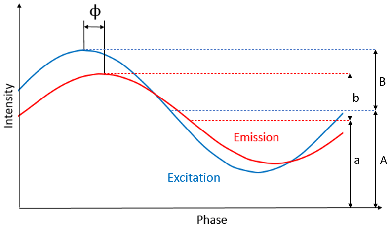
From Valeur and Berberan-Santos (2012) it is known that a material which is excited with a laser pulse signal, emits a maximum fluorescence intensity of I₀ at the time of the first radiation energy release. This intensity decays exponentially with the time t and converges to 0. The fluorescence lifetime τ represents the time period after which the fluorescence intensity I has decayed by $\mathrm{1}/e$ (see Fig. 1).

Figure 1 Illustration of the fluorescence decay characteristic.

On the basis of the system theory, the fluorescence excitation can not only be done by an excitation pulse (Dirac pulse) in the time domain but also by a Fourier transform test function, such as a sinusoidal or a rectangular oscillation with a defined modulation frequency ω. There are different possibilities to provide the excitation with a light source. Lasers and their high-power electronics are synchronized with the detection unit. Since the excitation varies in intensity but never breaks off completely, excited electrons are always present, the so-called steady-state population. The fluorescence signal follows the sinusoidal excitation with a phase shift ϕ. Additionally, the fluorescence exhibits the same frequency as the excitation signal but is attenuated in its amplitude and shifted in its direct current (DC) value. This attenuation arises from the material-specific quantum efficiency, which is smaller than 1. In Fig. 2, the amplitude of the excitation B, the amplitude of the fluorescence emission b, the DC value of the excitation A and the DC value of the fluorescence emission a as well as the phase shift ϕ are marked.

Figure 2 Illustration of the phase shift and the amplitude attenuation.

A calculation of the modulation depth M is possible using the ratios of the amplitude attenuation and the DC shift:

$$\begin{array}{}\text{(1)}& M={\displaystyle \frac{\left(\frac{b}{a}\right)}{\left(\frac{B}{A}\right)}}.\end{array}$$

Using the modulation depth M and the defined modulation frequency ω, the modulation-dependent fluorescence decay time τ_M, can be calculated

$$\begin{array}{}\text{(2)}& {\mathit{\tau }}_{\mathrm{M}}={\displaystyle \frac{\sqrt{\frac{\mathrm{1}}{M^{\mathrm{2}}}-\mathrm{1}}}{\mathit{\omega }}}.\end{array}$$

With the defined modulation frequency ω, the phase shift ϕ can be used to calculate the phase-dependent fluorescence decay time τ_Ph:

$$\begin{array}{}\text{(3)}& {\mathit{\tau }}_{\mathrm{Ph}}={\displaystyle \frac{\mathrm{1}}{\mathit{\omega }}}\times \tan \left(\mathit{\varphi }\right).\end{array}$$

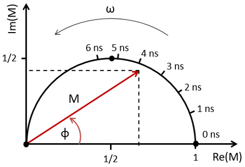
The measured parameters of M and ϕ can also be graphically displayed in a phasor plot, whereby M represents the length of the vector and ϕ the angle which M is rotated about the origin. The real part (Re) and the imaginary part (Im) of the modulation depth M are plotted along the x-axis and the y-axis. It contains a normalized unit circular axis, whereby the scaling of the fluorescence lifetimes are dependent of the modulation frequency ω. The phasor plot directly allows an evaluation of fluorescence lifetimes calculated from different measurements in comparison to each other (see Fig. 3).

Figure 3 Illustration of the phasor plot (Wohlschläger et al., 2020).

2.2 FD-FLIM measuring system

The determination of the fluorescence decay time is performed with the experimental setup used in Leiter et al. (2021). A frequency domain fluorescence lifetime imaging microscopy (FD-FLIM ) camera, a laser and a microscope to guide the laser beam onto the sample are the main elements of the experimental setup (see Fig. 4). The laser timing is controlled by the camera and provides a rectangular intensity-modulated excitation signal with wavelengths of either 405 or 488 nm. The light signal is coupled into the microscope via an optical fibre. The phase-shifted fluorescence response signal is captured by the magnifying objective and then detected by the FD-FLIM camera mounted on the microscope. The FD-FLIM camera has a resolution of 1004×1008 pixels and thus collects 10⁶ fluorescence lifetimes in parallel. Additional optical filters are used to confine the signal (exciter) and block unwanted reflections and stray light (emitter). The measured data are transferred from the camera to the computer via a USB 3.0 interface. The software processes the data and computes the fluorescence decay times of the wood samples.

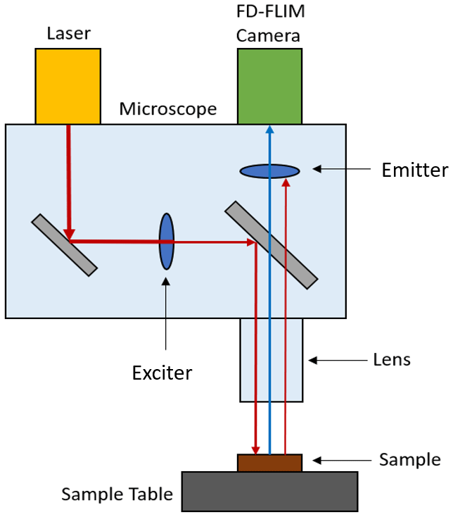
Figure 4 Illustration of the experimental setup used for the experiments including a laser, a microscope, optical filters and an FD-FLIM camera system.

3 Experiment

In the following, the wood samples are presented as well as the experimental setup and the two evaluation methods, first for the identification of the wood species and second for the identification of the post-consumer wood category.

3.1 Samples and data preparation

Standardized wood samples of maple, beech, oak, spruce, larch and pine were used for the identification of the wood species. The standardized wood samples were cut into blocks of 2 cm × 2 cm × 2 cm to investigate three sides (tangential, radial and transverse cut) of each wood type. Prior to the measurement, the standardized wood samples were preserved in a climatic chamber at a constant humidity of 60 % and a temperature of 25 ^∘C. A total of 16 fluorescence lifetime images were taken on the 3 sides of the wood samples using the measurement setup shown in Fig. 4 for each excitation wavelength (405 and 488 nm). This resulted in a total number of 288 measurements per excitation wavelength. The mean value and the corresponding standard deviation were calculated from the 16 measurements per surface of a sample by the Gaussian analysis described in Wohlschläger et al. (2020). The mean value was treated as an estimated value for the expectation value for every wood species. This resulted in three expectation values for the phase decay time and the modulation decay time of a wood species depending on the cutting direction of the surface.

For the investigations of the post-consumer wood category identification, eight samples of the category A1, nine samples of the category A2, one sample of the category A3 and one sample of the category A4 were collected from the material flow of a roofed post-consumer wood utilization plant. These samples were measured four times each using the measurement setup shown in Fig. 4 with 405 and 488 nm. This resulted in a total number of 76 measurements per excitation wavelength. The mean value and the corresponding standard deviation of the phase decay time and the modulation decay time were calculated from the measurement data for each measurement.

All measurements of the standardized wood samples and the post-consumer wood samples as well as the storage of the post-consumer wood samples were performed in a laboratory air-conditioned to room temperature of 23 ^∘C.

Figure 5 Flow chart of the evaluation decision tree to identify the wood species.

3.2 Identification of wood species

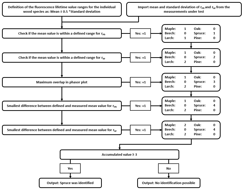
The main target was to develop a decision tree for the evaluation of FD-FLIM measurement data for the identification of wood species. Two main features of the FD-FLIM measurement are the phase-dependent and the modulation-dependent fluorescence decay times. Since these are material-specific, it is assumed that they differ depending on the wood species. The following analysis was based on the mean value of the phase-dependent and the modulation-dependent fluorescence lifetime of FD-FLIM measurements as well as on the associated standard deviations assuming a Gaussian normal distribution and the resulting phasor plot. As a basis for the evaluation, a library was created which contains the expected values for each wood species. As shown in Fig. 5, each measurement to be evaluated was subjected to five individual tests, whereby each one covered the six types of wood species previously mentioned. If a test fitted a wood species, it was registered in a point-based system. Once all individual results have been determined, the sum was compared to be greater than or equal to three to verify if the data belong to one wood species only. If so, this wood species was given as the overall result. If no wood species or several wood species had a decision value greater than or equal to three, no clear statement on the wood species assignment was possible.

For an analysis of the algorithm, the correct samples identified for the partial tests were compared, as well as the overall output of the decision tree with respect to the excitation wavelength.

3.3 Identification of wood categories

In addition to the wood species identification procedure, a decision tree for the identification of the post-consumer wood category A1 was developed. As possible classifiers, the parameters that have already been introduced for the wood species identification were considered. During the investigations a remarkable behaviour of the parameters was observed: the decay times of phase and modulation as well as the standard deviation of non-treated wood were often lower in comparison to treated wood of the same species. It is assumed that the composition of the treatment material affects the overall fluorescence decay time. Based on this knowledge, a decision tree was developed which processes the following measurement data: the mean value of the phase decay time, the associated standard deviation assuming a Gaussian normal distribution and the mean value of the modulation-dependent fluorescence decay time. The parameter value ranges vary as the excitation wavelength changes.

Figure 6 Flow chart of the evaluation decision tree to identify the wood category.

The test parameters were determined through the following procedure. The previously measured standardized wood samples for the identification of the wood species represented untreated wood, i.e. wood of the category A1. In combination with the observations during the post-consumer wood measurements the lower threshold value of the phase decay time was therefore set as equal to the shortest decay time including the standard deviation from the expected values obtained for the standardized wood samples. To determine the upper threshold value of the phase decay time, the longest decay time including the standard deviation from the expected values was set as the upper limit and the 72 post-consumer wood measurements were tested for this range. The test was repeated with the upper threshold lowered in steps of 0.1 ns until the range with the smallest error rate was found. This was repeated analogously for the modulation decay time. In addition, this procedure of reiterating the upper threshold of the phase and modulation-dependent decay time was repeated for the second excitation wavelength. To determine the parameters' standard deviation of the phase decay time, the smallest and the biggest value of the standard deviation of the decay time from the standardized wood samples was extracted. In this range the 72 post-consumer wood measurements were again tested varying the limit of the standard deviation in steps of 0.01 ns until the minimum of the error rate was found. In Fig. 6 the evaluation decision tree for the identification of the wood category consisting of three partial tests including the resulting parameters' value depending on the excitation wavelength are shown.

If two of the three individual tests were true, then category A1 was the result for the individual measurement. Otherwise, A2–A4 was the determined category. Since each sample included four individual measurements, the sample was considered to be category A1 if the results of each of the individual measurements were exclusively indicative for A1. In order to analyse the evaluation procedure, key indicators like the accuracy, precision and recall were calculated from the output (Powers, 2011). The accuracy was calculated as the sum of correctly identified A1 wood and correctly identified non-A1 wood divided by the total of the classified results. The accuracy gives an overview of the correctly predicted output. The precision was calculated as the ratio of wood correctly identified as A1 to the total amount of wood identified as A1. A high precision is required in order to achieve a high quality of the designation as A1 post-consumer wood. The recall was calculated as an ratio of those woods correctly identified as A1 divided by all A1 wood and should be high.

4 Results

The intention of the research was to evaluate the identification of wood species and wood categories by their fluorescence lifetime. In the following discourse the results of the investigation are provided and discussed.

Table 1 Results of the individual tests of the wood species identification.

4.1 Experimental results of the wood species identification

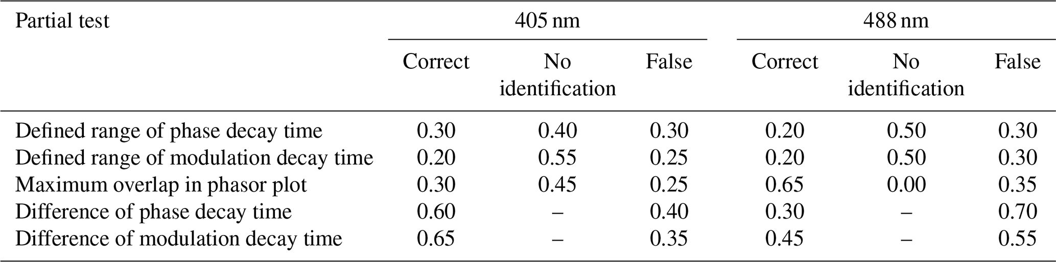
To identify the wood species, 20 fluorescence decay time measurements were randomly chosen out of the pool of 288 measurements. All measurements were taken from untreated wood samples where the wood species were known. Afterwards, the measured data were analysed using the previously explained procedures and the results were compared with the expected wood species. The proportions of correct results of the partial tests in relation to the excitation wavelength are shown in Table 1.

Table 2 lists the overall results depending on the excitation wavelength.

Table 2 Output of the wood species identification.

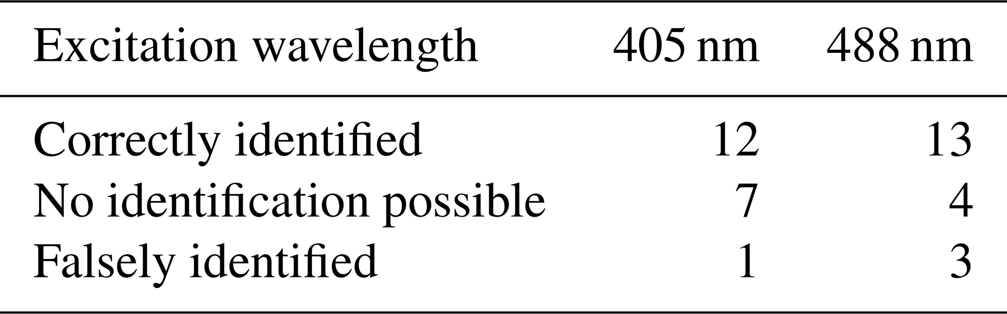
Although Table 1 reveals that the samples cannot be clearly identified by the individual tests alone, the combination of the five tests was successful. For an excitation with the 488 nm wavelength, the wood species were correctly identified in 13 out of 20 cases as shown in Table 2. In three cases, an incorrect wood species was obtained and no clear identification was possible in another four cases. Overall, a proportion of falsely identified wood species close to 0 should be aimed for. The results indicate that the wavelength 405 nm is more suitable for wood sorting because only one sample was incorrectly identified; however, even with this comparatively low error rate, the proportion of unmatched measurements was very high. It is considered that a further development by developing a neural network could increase the effectiveness of the method.

4.2 Experimental results of the wood category identification

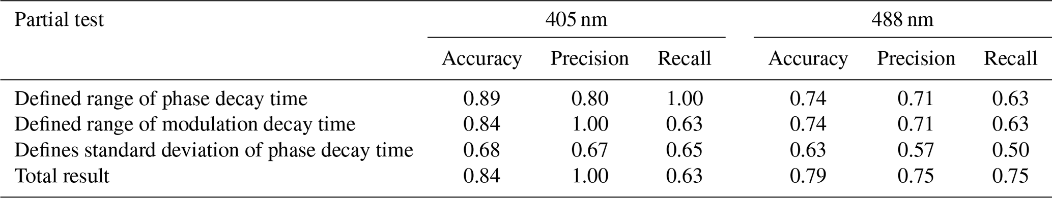
In addition to the identification of the wood species, this study analysed the identification of the wood category based on the fluorescence behaviour. For this purpose, 8 wood samples of category A1 and 11 wood samples of categories A2–A4 were examined according to the previously described method. Afterwards, the earlier explained evaluation process was applied. The results of the individual tests are shown in Table 3 with the accuracy, precision and recall values.

Table 3 Results of the individual tests of the wood category identification.

The overall results of the evaluation are shown in Tables 4 and 5 for the excitation wavelengths 405 and 488 nm, respectively.

Table 4 Output of the wood category identification for 405 nm.

Table 5 Output of the wood category identification for 488 nm.

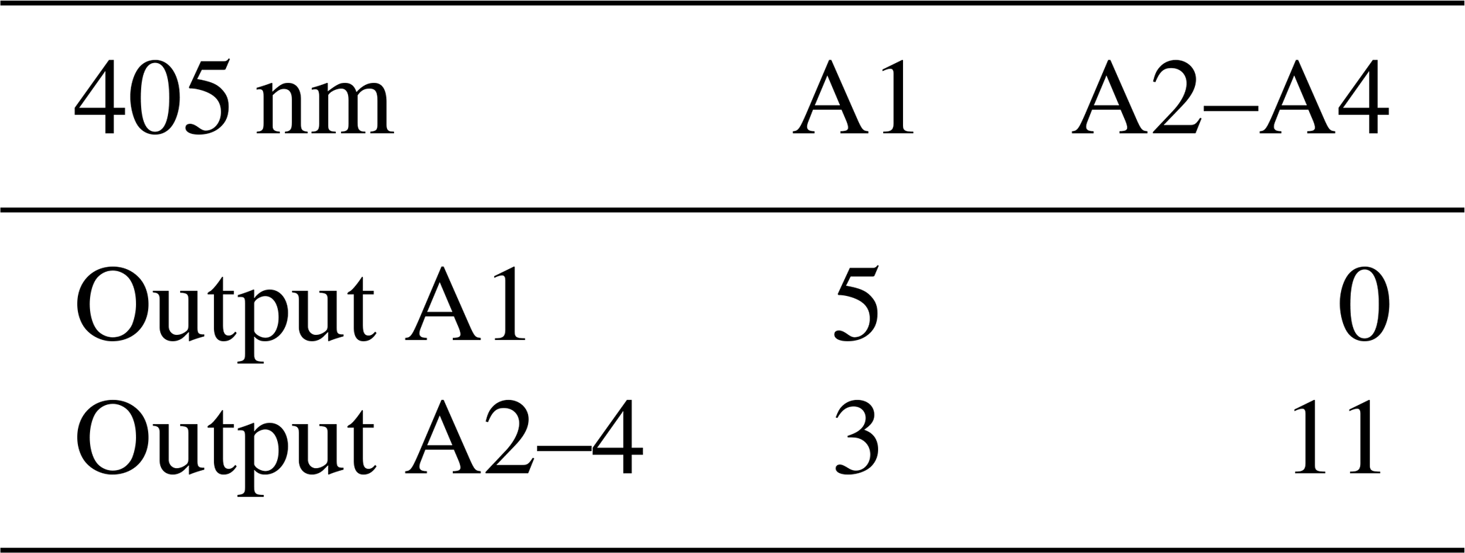
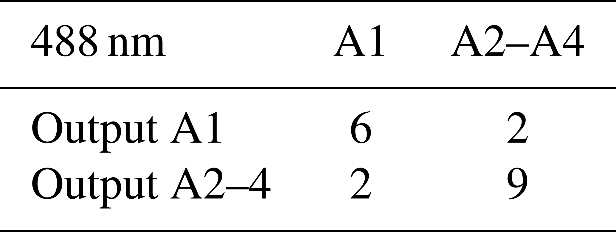
The values in Table 3 indicate that the use of an excitation wavelength of 405 nm yields a significantly higher accuracy. The parameter of the defined range of the modulation decay time leads to a high precision and the parameter of the defined range of the phase decay time leads to a high recall; however, the accuracy, precision and recall of the parameter of the standard deviation of the phase decay time are too low to be considered as a significant parameter. In the case of the excitation wavelength of 488 nm in Table 5, six wood samples were correctly identified as category A1 and nine wood samples were correctly identified as category A2 to A4. A total of two wood samples were incorrectly identified as category A2 to A4 and two wood samples were incorrectly identified as category A1. The values in Table 4 have to be interpreted in analogy for the excitation wavelength 405 nm. For industrial use, it is essential to eliminate the carry-over of pollutants. Therefore, a false identification of category A1 must be excluded in an automated process. With respect to the excitation wavelength 405 nm, this requirement has been achieved in this experiment. This leads to the assumption that a sorting of waste wood by post-consumer wood categories based on the fluorescence behaviour is very promising.

4.3 Results and discussion

The applied method, particularly in combination with the excitation wavelength of 405 nm, is very promising for wood sorting. A total of 12 out of 20 wood samples were correctly identified and only 1 wood sample was incorrectly assigned; however, the number of unassigned wood samples was quite high, which currently limits the effectiveness of the technique. Further experiments with larger sample sizes are required to improve the statistical resolution and repeatability. A greater amount of data will increase the statistical confidence and will bring the desired success. For the identification of post-consumer wood at an excitation wavelength of 405 nm, 16 out of 19 wood samples were assigned to the correct category. Only three of the A1 samples were incorrectly categorized as A2–A4 which is not critical for the recycling purpose of A1. This indicates a high potential of the FD-FLIM technique for post-consumer wood classification. The investigations showed that an identification of the wood category by a data-based decision tree is possible. For an improvement additional steps should be implemented in the method. For example, the threshold values can be fine-tuned and the intensity normalized to the exposure time, can be added as a parameter. In addition, all combinations of the parameters applied so far should be compared in order to find the most suitable combination. Overall, the drawback of the decision tree method are fixed decision thresholds. In a more sophisticated approach, the parameters and the uncertainty have to be properly weighted. The evaluation of the measurement data and the execution of the decision trees have so far been carried out in time-consuming manual steps. For a completely automated identification system, the decision tree has to be implemented in a computer programme. The extension of the data analysis to a data-based neural network will accelerate the classification process and will also lower the error rate due to an accurate parameter setting and the ability to consider all given values of the camera rather than the mean value and standard deviation of the decay time.

5 Conclusion

To date, there is no automated method for post-consumer wood sorting. Previous investigations demonstrated that the wood species can be identified due to their characteristic fluorescence decay times. In this contribution, it was demonstrated that a classification of post-consumer wood based on areal fluorescence lifetime measurements is possible using an FD-FLIM camera and laser diodes providing excitation wavelengths of 405 or 488 nm. The obtained data sets were evaluated by decision trees in order to identify the wood species and the post-consumer wood categories. The wood species tested were maple, beech, oak, spruce, pine and larch as well as post-consumer wood of the categories A1 and A2–A4. By using a decision tree and an excitation wavelength of 405 nm the wood species identification was successful for 12 out of 20 samples. By using a decision tree and an excitation wavelength of 405 nm, the post-consumer wood classification of 19 samples led to an accuracy of 0.84 and a precision of 1.00. Thus, the results revealed the high potential of the FD-FLIM technique with an excitation wavelength of 405 nm for wood sorting. Based on this knowledge, an automated process of fast post-consumer wood sorting seems feasible, which will increase the percentage of materially recycled post-consumer wood and will minimize the carry-over of pollutants.