the Creative Commons Attribution 4.0 License.
the Creative Commons Attribution 4.0 License.
 | 26 Aug 2022
Influence of the operation strategy on the energy consumption of an autonomous sensor node
Florian Schösser
Florian Schmitt
Eckhard Kirchner
Richard Breimann
Motivated by the application of industry 4.0 and Internet of Things (IoT) technologies, the development of cyber physical systems (CPS) is gaining momentum. As CPS require multiple measurement technologies to drive the intended function, e.g., condition monitoring and in situ measurement, the integration of measurement systems into industrial processes or individual products becomes a critical activity within the development process. Development methods like the V-Model support developers with methodological guidelines, but the related methods and models do not provide sufficient information regarding the energy supply of embedded systems. If the measurement system, consisting of sensor, calculation and communication unit is integrated inside an either sealed or moveable system, e.g., in a gearbox, ensuring a reliable communication and energy supply is a challenging task. This contribution therefore focuses on the energy supply, in particular the electric power consumption of autarchic measurement systems, referred to as sensor nodes. Based on a literature review of existing physical principles determining the energy consumption of semiconductors, a simple estimation model is derived. Estimation models in the current literature mainly focus on the effects of source code or software in general without analyzing a possible impact of operation strategies, such as generic data processing logics in practical applications. The model presented in this contribution is therefore used to identify the energy consumption of sensor nodes influenced by ambient and operating conditions of sensor nodes. Strategies are examined experimentally using an exemplary sensor node, a climatic chamber and a sensor-integrated gearbox as the system to be observed. An analysis of the conducted experiments leads to a more precise model, which is evaluated regarding its significance for predicting the energy consumption and the underlying simplifications. Finally, general relations influencing the energy consumption are presented and necessary research suggested.
- Article
(3146 KB) - Full-text XML
- BibTeX
- EndNote


Due to the development of intelligent systems in mechanical applications, it is beneficial to integrate sensors into machine elements to measure different phenomena directly in the process (Kraus et al., 2021; Vorwerk-Handing et al., 2020). A promising approach to integrate measurement functions is the use of sensing machine elements as design elements (Kirchner et al., 2018; Schork et al., 2016; Vorwerk-Handing et al., 2018). Most commonly used sensors are based on effects that lead to changes in the electrical behavior of a component. For using such a sensor an electric power supply is required, which makes a wireless charging method for the application in moving components necessary. Another possibility is to optimize the sensors behavior in a way that the energy consumption is minimized and the device can be supplied by an integrated life-long battery in the moving parts. Furthermore, energy harvesting approaches are a possible solution. In any case, the energy consumption of the sensor node must be estimated for any operating conditions to ensure its' supply.

Besides the energy for the sensor, signals must be transmitted to a reading system. Therefore, mostly wireless methods must be used due to the movement of components or placing of the components. This also is a surplus for the assembly of the components, but wireless technologies need a high amount of energy depending on the radio frequency which is proportional to the size of the transmitted data packages (Sultan et al., 2011). In order to achieve the most efficient transmission, only information relevant for the human-machine interface or the controlling system should be sent. It is therefore necessary to save data during processing to analyze the sensor data inside the moved components by comparing different sensor data. Therefore, besides the sensor, a calculation system like a microcontroller with a chip and a SD card as data storage unit is also necessary. The measured data are processed at the microcontroller and only relevant data are converted into the process information.
A sensor node is an electrical network consisting of one or more sensors to collect data and an electric calculation system like a microcontroller to convert the signal into the relevant process information. In this contribution, an autonomous sensor node is defined as a sensor node without a cable connection for power supply and communication. The autonomous sensor node consists of an electricity power supply and a contact-free communication unit (Zahhad et al., 2015).
To design this sensor node it is important to determine how much energy is necessary to run the whole sensor node including the sensor, an analog-to-digital converter and a microcontroller. As will be discussed later in this contribution, it is not the power but the total energy consumption for a given time that is the critical parameter for designers. An energy source, e.g., a battery, must be able to supply the node throughout the intended operation time. The energy consumption of autonomous sensor nodes can be estimated using models available in the current literature (Konstantakos et al., 2008; Ruberg et al., 2015). However, the relation between the energy consumption of a specific sensor node and its operating strategies as well as ambient conditions remains uncertain. Throughout this contribution a simple estimation model is derived from a literature review presented in the following section as well as additional research. The model does not need to calculate the power consumption exactly, but it should enable a mechanical engineer to approximately calculate the necessary power supply for the intended sensor operation. The model is tested using a sensor node based on Fig. 1.
In the following section the dominant effects influencing the total energy consumption of the sensor node are presented. Driven by the need to focus, only basic phenomena which affect the energy consumption, are presented, e.g., Ohm's law or the properties of semiconductors. The objective is not to derive an equation describing all parameters influencing the energy consumption but to generate a model based on effects that are determined by design or process parameters designers can influence. This model represents the qualitative relationship to the ambient conditions and allows an approximate calculation of the energy consumption based on the conditions in a given case.
2.1 Ohms law
Every part of an electric circuit shows ohmic behavior. The determining property of the ohmic response is the ohmic resistance, which is transforming electric power to heat. Equation (1) describes the relation between power P, voltage U and current I:
The resistance R depends on the material and geometry of the conductor as well as the operating temperature:
In Eq. (2) R20 describes the electric resistance at a temperature of 293.15 K or 20 ∘C, α20 the material-dependent temperature coefficient, ϑ the absolute temperature, ϑ20 the reference temperature at 20 ∘C in Kelvin, ϱ20 the specific electric resistance at a temperature of 293.15 K or 20 ∘C, l the length of the conductor and A the cross-section of the conductor (Weißgerber, 2018).
Figure 2Three-dimensional fin structure of a transistor based on Han and Wang, 2013.
2.2 Semiconductor theory
Today microprocessors are based on the fin field-effect transistor technology (FinFET), allowing high calculation power with small surface and a low energy consumption. The process operates like the common metal oxide semiconductor field-effect transistor (MOSFET), but the use of three-dimensional fin structures (Fig. 2) allows placement of a higher number of single transistors on a same size chip (Han and Wang, 2013).
The MOSFET consists of two transistors with different doping to block each other for saving energy. The energy consumption of microchips is characterized by the leakage current, which can be summarized in the following equation (Zhang et al., 2003):
The leakage current shows a complex relation to a lot of different parameters. In this contribution the authors focus on how an engineer can influence the energy consumption of available chips so the individual parameters will not be explained in this article. Additional information can be found in the referred literature. The thermal voltage consists of the Boltzmann constant kB, the ambient temperature ϑ and the elementary charge e. The threshold voltage UT is also a function of the temperature, but can be approximately described by a linear relation (Zhang et al., 2003). The modeling objective is to derive a simplified model for the leakage current, which is reduced to parameters developers can influence. The only possibility besides the choice of the chip is to change the position of the microcontroller and influence then the ambient temperature. The following equation shows the simplified equation:
Another important point is the examination of the calculation process on the level of a transistor in a switching process, which occurs periodically with the operation frequency of the transistor. The corresponding part of the energy consumption will further be referred to as dynamic power consumption Pdyn.
The power loss of the leakage current also depends on the drain voltage of the transistor UDD and is independent of the operation frequency. Another relevant part is the electric current during the switching process, where for a short time both transistors drive a current (Helms et al., 2004). To quantify this, a mean current is calculated by integrating the current over the period . The gain factor β depends on the geometry, the capacity and number of transistors in one chip (Veendrick, 1984). The drain voltage UDD, the threshold voltage VT and the rise and fall time τ of the inverter depend on the chip design and cannot be influenced by the user (cf. Eqs. 5 and 6).
Another significant power loss is the charging process of the transistor gates, which show capacitive behavior. The loading power is characterized by the capacity of the power node CL, the node voltage UDD and the frequency f.
The following equations summarize the three sources of power dissipation in digital complementary metal oxide semiconductor (CMOS) circuits:
The authors know there are more phenomena influencing the CMOS process and therefore the power consumption, but as the objective of this contribution is to build up a simple model usable without detailed knowledge of semiconductor processes, other phenomena are neglected as designers cannot influence their impact on the overall energy consumption. The dynamic power consumption only depends on the chip frequency and can be simplified to . The power consumption for writing the data into the data space is not explicitly mentioned in the theory because the data are only saved in the working space. Only the interesting information is saved on the SD card, so authors assume small amounts of data in general. The saved data per test cycle of 10 min are very small (approx. 600kB per test cycle) and the energy consumption of comparable SD cards as analyzed in a sensor node in Kombo et al. (2021) is much smaller, approx. 4 %–5 % of the frequency-dependent energy consumption of the chip and will take place in only approx. 6 ms of the chip's processing time (10 or 5 min).
2.3 Energy consumption model
After evaluating the available energy consumption models the scope of this contribution is refined. Ortiz and Santiago (2008) pointed out that the energy consumption of embedded systems is highly dependent on the implemented source code, whereas contributions like Gotz et al. (2020) addressed the correlation between levels of voltage and frequency supplying the embedded system and the resulting power consumption. Moreover, the models in the current literature suggest a significant impact of sleep mode and data logging power consumption. Thus, this contribution addresses the need of a model representing the effects of operating strategies as a combination of different operation modes as well as operating conditions such as ambient temperature. The CPU frequency, which is central in the experiments of Gotz et al. (2020), is only used as a parameter to distinguish between the operation strategies and explain the different energy consumptions.
By summarizing all factors that are influencing the power consumption and reducing the parameters that depend on the chip design, there are only two parameters left, which can be analyzed in terms of their quantitative effect on the overall power consumption: the ambient temperature and the frequency. A higher temperature does not necessarily lead to a higher energy consumption because the leakage current depends, besides the quadratic multiplication, also on the temperature in the numeration of the exponent function. The power loss shows a linear increase with higher frequency due to the higher amount of switching and charging processes of the gates. It is also necessary to mention that the sensor node consists of more electric devices than the semiconductor material in the chip, so the ohmic behavior with the temperature dependence also must be mentioned. All other variables and parameters depending on the transistors design are summarized to the factors W, X, Y and Z. These observations lead to the following model, where ϑ0 is defined as the absolute temperature at 0 ∘C in Kelvin:
This model will be used in a simplified form based on the experimental results to estimate the power consumption of the sensor node.
2.4 The quantitative working space model
In advance of describing a system, developers need to determine which modeling approach is suitable to achieve their modeling objective as it is hard to choose the right model. Therefore, contributions like Eisenmann et al. (2021) and Matthiesen et al. (2019) support practitioners by providing comprehensive reviews on existing models.
As one possible modeling approach, the quantitative working space model (qWSM) is presented. The qWSM separates a system in three-dimensional subsystems, so-called working spaces (WS), which can consist of solid bodies as well as fluids and are contained by their surfaces, so-called working surfaces (WSU). Interaction between WSs is possible only if two WSUs are in direct contact and therefore form a working surface pair (WSP) at which matter, energy, information, etc. can be exchanged. The qWSM evolved from the working space model (WSM) developed by Beetz et al. (2018) and Beetz and Kirchner (2019). Furthermore, the original WSM was inspired by the contact and channel approach (Albers and Wintergerst, 2014; Grauberger et al., 2020; Matthiesen et al., 2018) and the contact and channel model (Braun et al., 2009).
The characteristic difference to other system representations used in product development is that the qWSM is built up on the balance of conservation variables such as energy or charge to describe the behavior of WS and the coupling as WSPs. Linking the WSs by balance and coupling equations leads to a quantitative representation of the overall system. The qWSM generated can be used to analyze the effects of modifications in individual WS e.g., temperature on the behavior of the overall system or energy consumption of electric components and vice versa.
During the course of this contribution, a qWSM of the exemplary sensor node is used to relate the findings on existing influencing factors of the energy consumption to states of the WSs.
The research question motivating the following section is how engineers as users can benefit from the presented physical dependencies of the energy consumption. The authors decided to use a targeted varying to change the operating parameters and ambient conditions and analyze the behavior of the sensor node.
3.1 Definition of strategies for sensor nodes
The parameters ambient temperature ϑ and frequency f to be varied are selected based on the model represented by Eq. (7) As the frequency of a microcontroller depends on the calculation process used and cannot be easily influenced, it is necessary to figure out different operation strategies of the sensor node and measure the impact on the energy consumption.

3.1.1 Temperature
Designers can influence the ambient condition “temperature” of the transistors by the design of the insulation of the chip and the placement in the machine element. To analyze the impact of the temperature the authors decide to use a room temperature of 25 ∘C as a benchmark value and change to a higher temperature of 50 ∘C and a lower temperature of 0 ∘C during the experiments. The higher ambient temperature is set to 50 ∘C since the microcontroller used has a maximum operation temperature of 85 ∘C in the transistors. The maximum temperature of the transistors is higher than the maximum ambient temperature.
The lower temperature of 0 ∘C is the minimum temperature specified as ambient condition for the microcontroller used.
3.1.2 Frequency
The frequency depends on the measurement strategy and the implementation of the data processing. Therefore, the authors define three different strategies for how the measurement of the sensor data and the data processing can interact:
-
One data point is read and directly processed.
-
Data points are read constantly, saved and afterwards processed periodically in a fixed time cycle.
-
For a short period in a time cycle data points are read and directly processed, the node is set to a sleep mode before the next active period is started.
Prior to the experiments the authors assume for strategy 1 a nearly constant power consumption over time due to the similar workload over the whole measurement period. In the following the authors make a paired comparison to assume the energy consumption of the different phases of the other strategies (Saaty, 2008). The authors assume that strategy 2 will lead to lower central processing unit (CPU) frequencies in the phase of data measurement and collection due to a lower workload. This will lead to a lower dynamic energy consumption during this phase, whereas the energy consumption in the data processing time interval is expected to be higher. For strategy 3 the authors assume the same energy consumption in the data processing phase as in strategy 1 due to using the same logic. When the microcontroller remains in a sleep mode without dynamic power consumption a very low energy consumption is expected. It is mentioned that in the starting process the microcontroller must boot and will consume more energy for a short time. The assumptions are illustrated with their time dependency in Fig. 3.
Figure 3Assumed energy consumption of three different time-dependent strategies prior to the experiment.
It is important to point out that the implementation of strategy 2 ensures the collection and processing of the same amount of data like strategy 1 whereas strategy 3 will process less data.
3.1.3 Combined strategies
The derived strategies are tested using the set-up described in the following section. The objective is to analyze the dependence of the energy consumption on ambient temperature and frequency for the configurations specified in Table 1. Strategies 5 and 7 are variations of strategy 3 and focus on the impact of ambient temperature on static power losses. Therefore, it is also important to observe the influence on the temperature during sleep mode. Strategy 2 does not require experiments with different temperatures because the only difference to strategy 1 can be found in different CPU frequencies in the reading and calculation interval and therefore the dynamic power loss. Table 1 gives an overview of the combined strategies for the experimental set-up.
3.2 Experimental set-up
This section describes the set-up of the sensor node with the chosen components and its application system. Also, the implementation of the temperature-dependent and time-dependent strategies for the experiments are explained and the measurement strategy to identify the energy consumption of the sensor node is described. The set-up is designed following the requirements for prototyping presented by Schork and Kirchner (2018) in order to create knowledge enhancing the finding of Sect. 2.
3.2.1 Components
Driven by the requirement to limit the complexity of the experiments, it is necessary to set up the test rig using components available on the market. As presented in the fundamentals the dominant energy consumer of sensor nodes are semiconductors, which can be found in the CPU of microcontrollers. Therefore, a Raspberry Pi 4B with 8 GB RAM is used as an easy accessible and programmable calculation unit.
As an energy source a battery-supplied DC/DC converter is used and set to a constant input voltage of 5.2 V. To use analog sensor signals the authors added a specific sensor plate to the Raspberry Pi with an integrated analog-to-digital (A/D) converter. An analog speed sensor is integrated stationary in the gearbox and identifies the magnetic resistance of the rotating teeth. The working principle is based on the anisotropic magnetoresistive effect (Dietmayer, 2001). During the rotation of the gear wheel the sensor data show a sine-curve with one cycle per gear tooth. The authors decided to incorporate an implementation to calculate the rotation speed by analyzing the sensor data for extreme points (maxima and minima) by comparing following data points and analyzing the timeline of values.
A temperature chamber is used to realize the different temperatures. The experimental set-up is designed in a way that only the microcontroller with the A/D converter is placed in the heating chamber and all other parts like battery package or the DC/DC converter are outside. In doing so the temperature dependence of the microcontroller consisting of semiconductor materials and not the battery or the measurement set-up are examined and can be depicted in the model according to the experimental data. The developed model does not describe the effects of a temperature-dependent inner resistance of a battery or other components, thus they are operated at a constant ambient temperature.
3.2.2 Measurement strategy
The energy consumption is measured by a parallel arrangement of a shunt resistance and an oscilloscope in the electric circuit. The power consumption can be calculated by the voltage of the microcontroller UMC and the current IMC, which can be calculated by the voltage drop at the shunt Ushunt divided by its resistance Rshunt:
The voltage at the DC/DC converter UDCC is set to 5.4 V in operation mode to receive the input voltage of 5.2 V at the microcontroller. The difference of approximately 0.2 V is equal to the voltage drop at the shunt resistance and inevitable due to the potential dividing property of the electric circuit. The resulting electric circuit is shown in Fig. 4.
Moreover, it is important to analyze the processors' behavior during the data processing phases, which can be characterized by the frequency of the CPU. In doing so the dependence between the frequency and the dynamic power consumption can be identified and quantified. Furthermore, the core temperature of the CPU is measured as it influences the static leakage current. Both parameters are measured by the internal measurement system of the microcontroller. As the reliability of these parameters is a source of uncertainty, they are used to derive qualitative relations between the energy consumption and alternating temperature and CPU frequency. The CPU temperature shows a varying difference to the ambient temperature when operating the node in different ambient temperature levels. Therefore, it is essential to use the internal temperature as additional measurement to the controlled ambient temperature.
3.2.3 Implementation of the time-dependent operation strategies
For the experiments with operation strategy 3 it is necessary to save the data before the microcontroller is shut down and to avoid overwriting the parameters from the last interval. Therefore, a time-based if-condition is used. All operation strategies are tested for a period of 10 min. For strategy 2 the processing time interval is chosen as 60 s. For strategy 3 the shutdown period is set to 50 s. The implementation of strategy 2 realizes the measurement of new data during the data processing by a multiprocessing approach. The time interval in strategy 3 is shorter than 60 s to compensate for the starting and shutdown times. The booting process requires an external trigger signal. The implementation automatically initiates the measure and processing codes after its boot phase.
This section gives an overview of the experimental results for the different operation strategies and derives suggestions, which strategies can be used to reduce the energy consumption. Also, the simplified estimation model for the energy consumption is confirmed and specified for the sensor node used.
4.1 Comparing the experimental results of two equal sensor nodes
In order to improve the statistical significance of the gathered data all operation strategies are tested for two equal sensor nodes. To analyze the influence of the microcontroller and identify the product-individual electronic tolerance and their influence on the energy consumption in detail, a higher sample of at least 30 microcontrollers is necessary to get statistically independent results. The results of the energy consumption of the two microcontrollers show different offset values but a similar behavior over all operation strategies. Figure 5 shows an example data set of the measured voltage at the shunt resistance for operation strategy 1.
Both microcontrollers show an unexpectedly volatile behavior as the implementation is identical for every data point. The different workload of the CPU during the measurement and data processing leads to a volatile CPU frequency and as a further consequence to a volatile voltage drop, which explain the observed behavior.
4.2 Results of the time-dependent operation strategies
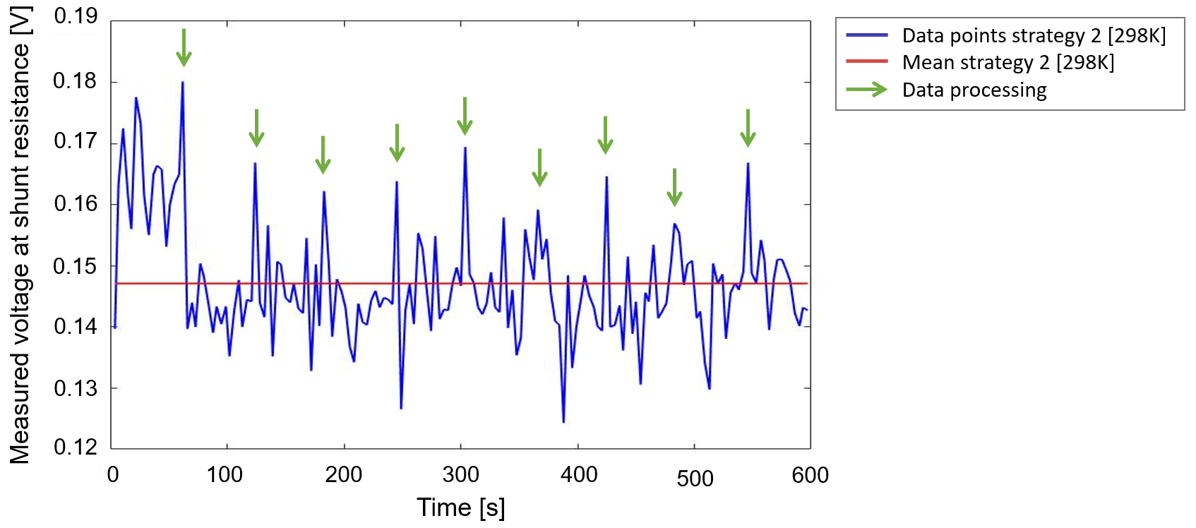
Operation strategy 2 shows a significantly reduced voltage drop and therefore lower energy consumption of the sensor node (cf. Fig. 6). This can be explained by the implementation as a loop and the ability of the processor to optimize its frequency for the further cycles. After time periods of approximately 60 s fluctuations to a significantly higher voltage drop are observed. They are limited to a duration of less than 1 s and occur during the data processing intervals.
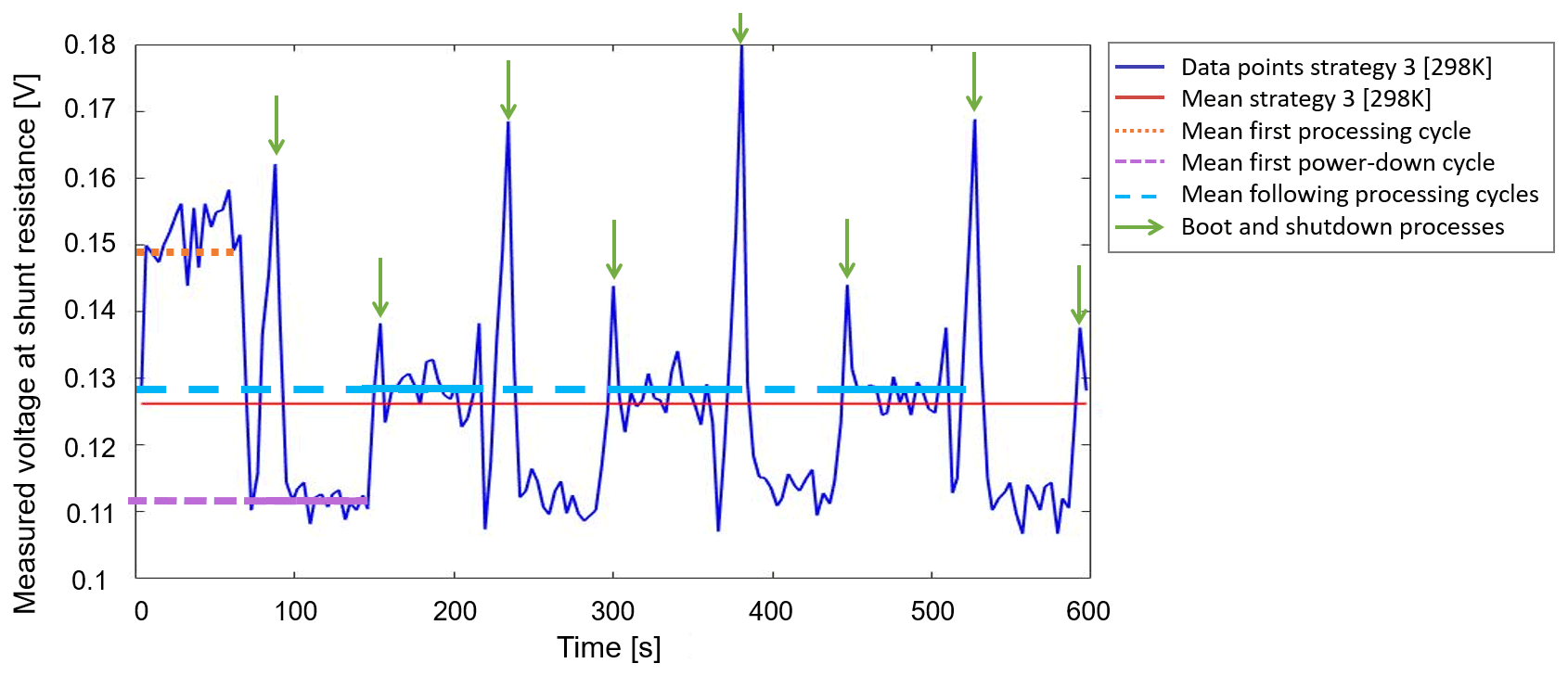
Operation strategy 3 in Fig. 7 shows a high voltage drop during the first cycle, which is reduced after approximately 60 s to a significant level for all following cycles. This behavior can be explained by the shutdown, but even during the assumed nonpower-consuming period the voltage drop with a value of 0.11 V is only 74 % of the active period and the energy consumption of the microcontroller must be at least 2.33 W.
Operation strategy 2 can reduce the energy consumption by up to 7 % while measuring and processing the same amount of data as strategy 1. The mean power consumption of strategy 3 is lower than of strategy 2. A significant limitation of strategy 3 is that less than 50 % of the data can be measured and processed compared to strategy 2 during the same operation time. Operation strategy 3 shows high power consumption in the boot and shutdown processes of the microcontroller. For this reason, the strategy is suitable if the application only requires a periodic measurement of data after long sleeping periods as both tested microcontrollers showed.
4.3 Results of the temperature-dependent operation strategies
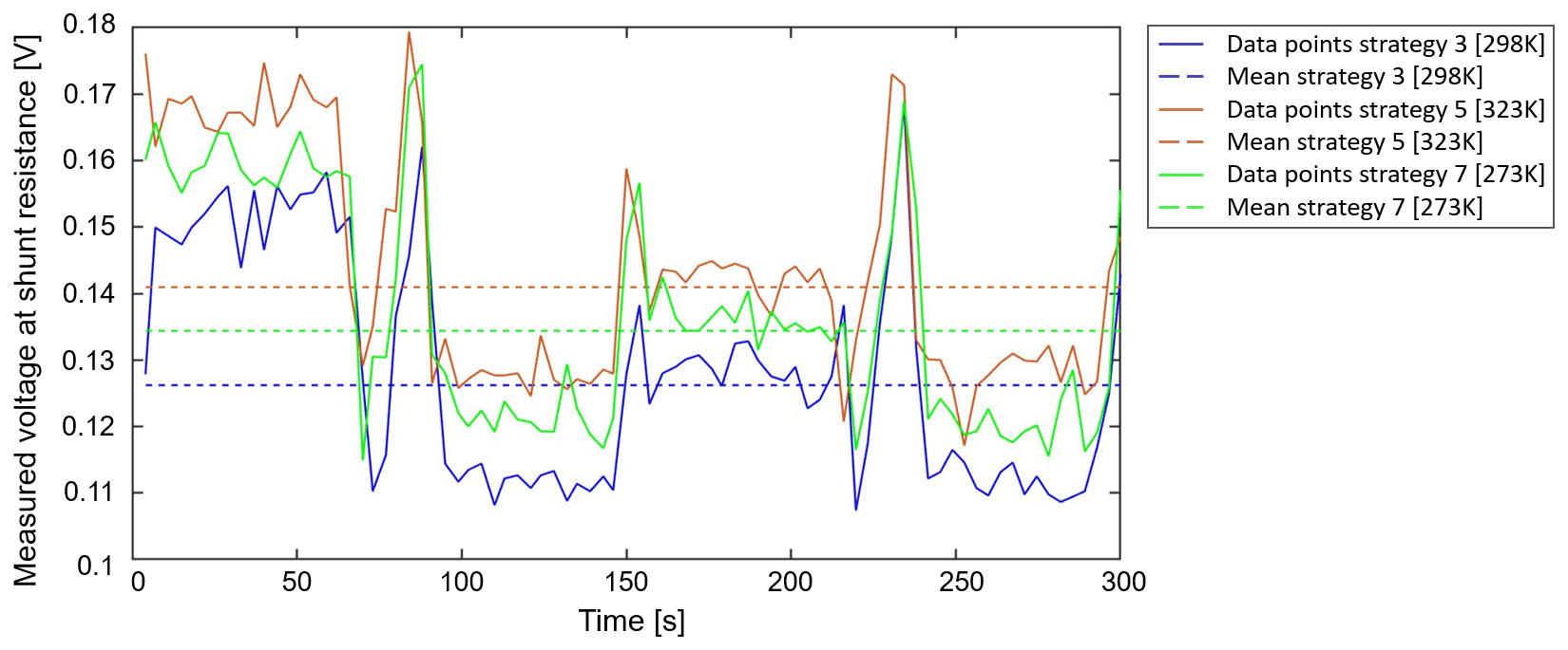
Figure 8 shows a temperature-dependent comparison of the corresponding time-dependent operation strategies 3, 5 and 7. To optimize readability the dataset is reduced to 300 s. The operation strategies 1, 4 and 6 show similar results.
As expected, the energy consumption at higher ambient temperature rises irrespective of the time-dependent strategy used. The power consumption at the lower ambient temperature is also higher than at room temperature at comparable CPU frequencies, which was not predicted by the estimation model. This cannot be explained by the static leakage current, so there must be another effect causing a higher energy consumption at lower temperature. This can be explained by the temperature coefficient α20 of the conductor material in the microcontroller. This material has a negative temperature coefficient so that a lower temperature will lead to a higher resistance and a higher power consumption (compare Eq. (1)). Due to the exponential character of the static power loss, it is comprehensible that this linear behavior superposes overall energy consumption at lower temperatures (compare Eq. (7)).
The benefit of using strategy 3 with shutting off the microcontroller has its biggest effect at room temperature with a lower power consumption of 0.614 W, whereas it is only 0.511 W at 50 ∘C or 0.531 W at 0 ∘C, as presented in Table 2. The similar CPU frequencies show a similar dynamic power consumption. A minimal consumption can be found close to room temperature with comparable low energy consumption influenced by the temperature-dependent resistance and the static power losses.
4.4 Analysis of the CPU frequencies
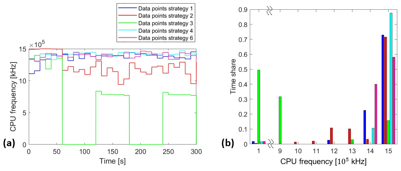
To quantify a possible dependence of the energy consumption on the frequency, the implementation records the CPU frequency of the microcontroller. Due to the theoretical model developed in Sect. 2, the authors expect a different CPU frequency for the time-dependent operation strategies, but equal frequencies for the variation of the temperature. Figure 9 shows extracts of the data and a calculated mean of the CPU frequencies.
For strategy 3 the mean is only calculated for the time intervals in which the microcontroller is in an active mode. It can be confirmed that the time-dependent strategies result in a different CPU frequency whereas the temperature-dependent strategies (4 and 6) show nearly the same CPU frequencies (as strategy 1) and confirm the expectation of the theory. Thus, the results show that the CPU frequencies are responsible for the differences in terms of energy consumption between the time-dependent strategies without considering the booting phase of strategy 3. As the CPU frequency can only be measured through the implementation code, which can only be started at the end of the booting phase, there is no information about the frequency during the booting process. Due to the differences in power consumption for the temperature-dependent strategies and nearly the same CPU frequency, it can be suggested that the temperature must have a relevant impact on the energy consumption of the sensor node. It can also be shown that strategy 2 has lower CPU frequencies compared to strategy 1, and is a reliable strategy to save energy.
4.5 Analysis of core temperature
Regarding the static power consumption, the state variable is the temperature of the semiconductor structures, or in the general calculation unit, which is higher than the ambient temperature. Especially when operating at room temperature the core temperature is approximately 25 ∘C higher. It can be observed that during active calculation processes the core temperature slightly increases over time. The strategy at the higher ambient temperature shows a similar behavior with a slightly minor temperature increase.
4.6 Calculation model
Based on Eq. (7) in Sect. 2.3 the dependence of energy consumption of a sensor node on the mean processor frequency and ambient temperature can be simplified to the following equation with the unknown parameters Kx:
A simple estimation model for a specific sensor node can be derived from Eq. (7) and adapted by calculating the unknown parameters from representative experiments. For a practical usability of the model, it is necessary to separate the energy consumption into the dynamic and the static parts. For the identification of the dynamic part, the authors use the measured energy consumption depending on the frequency of the measurements at room temperature. To calculate the factor of the linear dynamic dependency a second data point is required. To avoid influences by different phenomena in the time-dependent strategies a so-called off-set experiment is carried out. Here, the energy consumption of the sensor node is measured when the measurement and data processing code is not run. The linear regression gives the following equation:
It is important to mention that this relation differs a lot from values of the data sheet, which suggests a correlation of
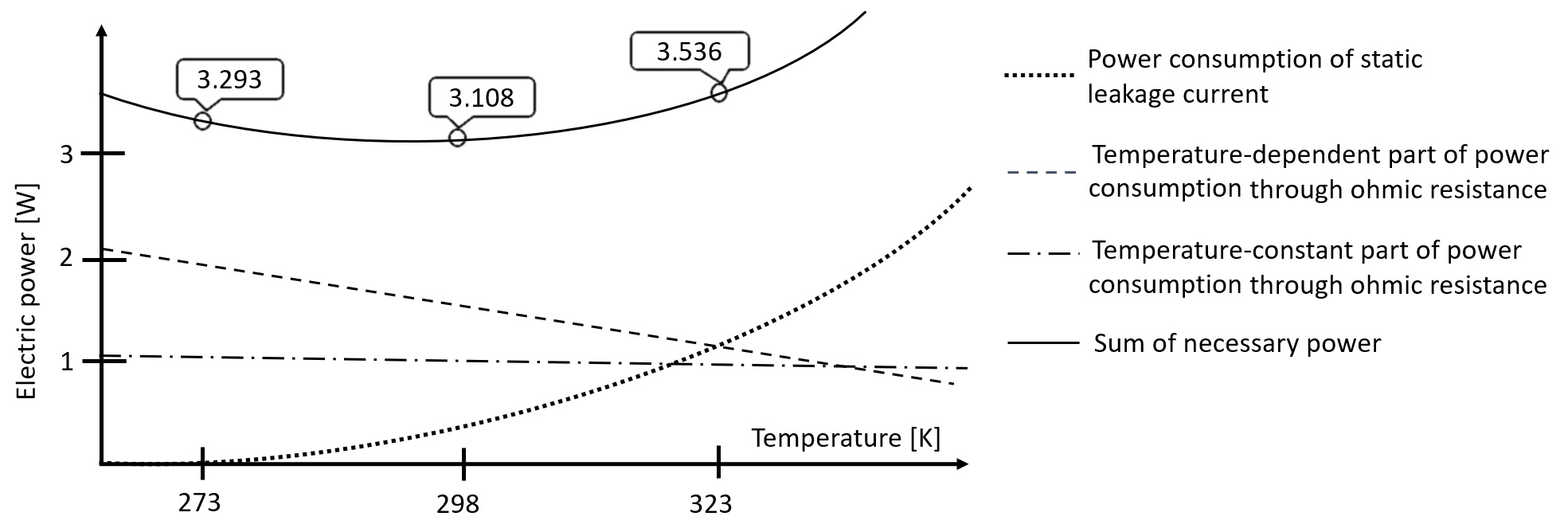
The authors want to point out the different results based on measurement and data sheet to show further need for research. Especially the comparably high power consumption should be analyzed to approve the suggested model. As presented in Sect. 2.1–2.3, the static power consumption can be calculated by a mathematical equation depending on the temperature. In this case a regression analysis is not sufficient. As illustrated in Fig. 10 the superposition of the decreasing ohmic power consumption and the increasing static power consumption of the microcontroller can be approximated by a quadratic function in the relevant range of temperature.
The approximation, compare Eq. (11), shows reliable results for a limited temperature range and enables designers to estimate the power consumption of a specific sensor node.
To calculate the regression parameters for the dynamic power consumption the authors use experimental results. The regression analysis is conducted for the ambient temperature as input variable. A user can adapt the model to the relevant temperature.
In order to unite the information of both equations, the authors calculate the energy consumption at 0 ∘C from the frequency-independent part at 25 ∘C by using the temperature model. This leads to a temperature and frequency independent energy consumption of 2.415 W. The resulting estimation model is
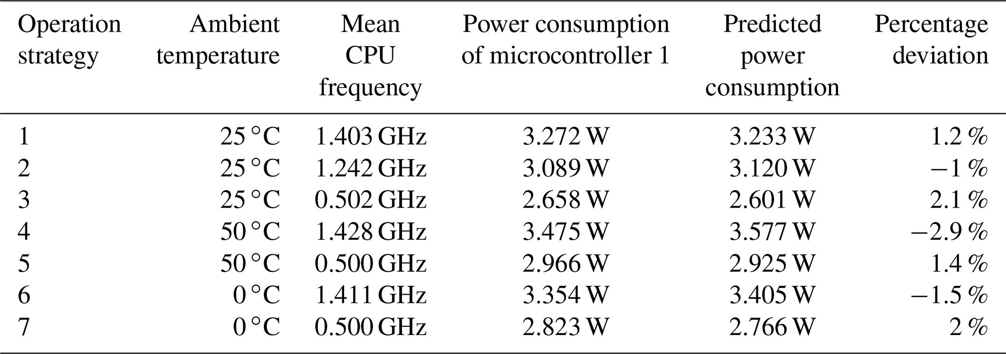
Table 2 shows a comparison between calculated and measured values of the energy consumption. The values deviate in a range of less than ±3 %, which is significantly less than the differences between two equal sensor nodes.
Table 2Overview of the measured and calculates energy consumption.
4.7 Integration into the quantitative working space model
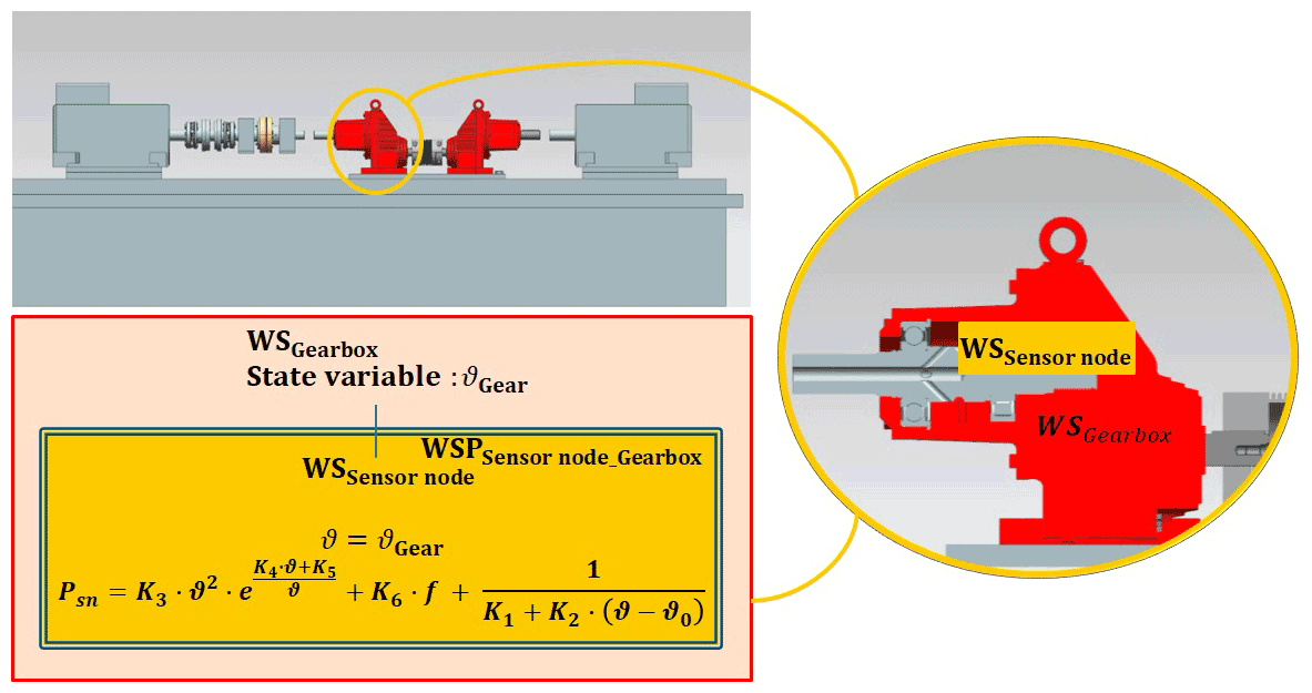
The derived mathematical description of the energy consumption can be integrated into a qWSM as a characterization of the WS “sensor node”. Designers can estimate the quantitative effects of ambient conditions and operation strategies on the energy consumption of an integrated subsystem. The used test rig and the resulting qWSM of the sensory gearbox is shown in Fig. 11. Using the developed estimation model cf. Eq. (13) the energy consumption can be evaluated on a qualitative as well as quantitative basis using a single representation of the system. Therefore, it can support the definition of suitable operation strategies meeting the super system's requirements regarding the node's energy consumption. Summarizing the aforementioned, the qWSM can be seen as a promising tool to support the integration of sensor nodes into technical systems.
The developed model extends the range of tools accessible to designers and empowers them to estimate the energy consumption of a sensor node e.g., for implementing sensory functions directly into the process of interest, meeting the requirements of industry 4.0, IoT, increasing connectivity and digitalization. The modeling objective was to analyze the dependence of the energy consumption on the chosen operation strategy and present ambient conditions of the sensor node. The resulting approximation model cf. Eq. (9) exceeds early approaches like Konstantakos et al. (2008) in terms of applicability to a specific development task that requires the integration of standardized microcontrollers. The model identifies the CPU frequency f of the calculating unit and the ambient temperature ϑ as determining parameters by analyzing the general physical effects in conductors and semiconductors in a sensor node. To quantify their effect ϑ and f are used as input variables for the model to design and optimize the energy consumption in early product development phases. Estimation models in the current literature like Gotz et al. (2020) or Ruberg et al. (2015) mainly focus on the effects of source code or software in general or components of the sensor node (Ruberg et al., 2015), whereas the derived model supports the estimation based on defined operation strategies as generic data processing logics in practical applications with only minimal adaptations of the source code.
The integration of the model into a qWSM enables engineers to design a life-long battery or a wireless charging solution for a specific sensor node based on a given data processing implementation and the ambient temperature at the sensor node's position. Designers can now evaluate different design solutions in terms of e.g., sensor position or insulation using the estimation model. By accessing different operation strategies, a strategy suitable for preliminary defined requirements can be derived. The limitations of the sensor node in terms of ambient temperature can be described on a quantitative bases using the qWSM. Experimental observations show advantages in the energy consumption of a strategy collecting and processing data in time intervals. The influence of the frequency and temperature could be shown by the experimental examination of a sensor node. The temperature-dependent effects on the ohmic behavior of the conductor and the behavior of the leakage current in the semiconductor material show higher energy consumption at higher and lower temperatures than room temperature. Further research needs to be conducted to derive a generalizable estimation model for sensor nodes as the presented model is adapted to one specific class of sensor nodes and the microcontroller used. The model uses some extensive simplifications in order to limit the complexity of adapting it to a specific sensor node. Nonetheless, the effects of these simplifications have to be investigated further to ensure a reliable estimation for various sensor nodes.
The implementation of the microcontroller serves as a representation of the operation strategies and can be provided for reproducing the experiments for a similar sensor node. All experimental data were analyzed using Matlab. The scripts for analyzing and visualizing the data can be provided on request.
All experimental data are available and can be provided on request.
FSchö developed the first iteration of the model and designed the experiments under the supervision of and in cooperation with FSchm as his final thesis. Both carried out the experiments and analyzed the data. FSchö further developed the model by integrating the findings of the experiments. FSchm prepared the manuscript with contributions from all co-authors. RB supported the preparation of the manuscript by putting the model into perspective of the integration in situ measurement functions. EK guided the research as head of the institute and derived the research question, which served as a motivation for the final thesis.
The contact author has declared that none of the authors has any competing interests.
Publisher's note: Copernicus Publications remains neutral with regard to jurisdictional claims in published maps and institutional affiliations.
The authors thank the Deutsche Forschungsgemeinschaft (DFG, German Research Foundation), which funded the presented research within the project “Opportunities and limits of the working space model in product development”.
This research has been supported by the Deutsche Forschungsgemeinschaft (DFG, German Research Foundation; grant no. 443578519).
This paper was edited by Rosario Morello and reviewed by three anonymous referees.
Albers, A. and Wintergerst, E.: The Contact and Channel Approach (C&C 2-A): Relating a system's physical structure to its functionality, in: An Anthology of Theories and Models of Design, Springer, London, 151–171, https://doi.org/10.1007/978-1-4471-6338-1_8, 2014.
Beetz, J.-P.and Kirchner, E: Das Wirkraummodell – Ein Hilfsmittel bei der Gestaltung sauberkeitsrelevanter Produkte, Forsch. Ingenieurwes., 83, 933–946, https://doi.org/10.1007/s10010-019-00375-0, 2019.
Beetz, J.-P., Schlemmer, P., Kloberdanz, H., and Kirchner, E.: Using the new Working Space Model for the development of hygienic products, in: Design Conference Proceedings, Proceedings of the DESIGN 2018 15th International Design Conference, 21–24 May 2018, Dubrovnik, 985–996, https://doi.org/10.21278/idc.2018.0142, 2018.
Braun, A., Albers, A., Clarkson, P., Enkler, H.-G., and Wynn, D.: Contact and channel modelling to support early design of technical systems, in: Proceedings of the 17th International Conference on Engineering Design (ICED'09), 24–27 August 2009, Stanford, https://www.designsociety.org/publication/28681/Contact+and+Channel+Modeling+to+Support+Early+Design+of+Technical+Systems (last access: 19 August 2022), 2009.
Dietmayer, K. C.: Magnetische Sensoren auf Basis des AMR-Effekts (Magnetic Sensors Based on the AMR-Effect), Technisches Messen, 68, 269–279, https://doi.org/10.1524/teme.2001.68.6.269, 2001.
Eisenmann, M., Grauberger, P., and Matthiesen, S.: Supporting Early Stages of Design Method Validation: An Approach to Assess Applicability, Proc. Design Soc., 1, 2821–2830, https://doi.org/10.1017/pds.2021.543, 2021.
Gotz, M., Khriji, S., Chéour, R., Arief, W., and Kanoun, O.: Benchmarking-Based Investigation on Energy Efficiency of Low-Power Microcontrollers, IEEE T. Instrum. Meas., 69, 7505–7512, https://doi.org/10.1109/TIM.2020.2982810, 2020.
Grauberger, P., Wessels, H., Gladysz, B., Bursac, N., Matthiesen, S., and Albers, A.: The contact and channel approach – 20 years of application experience in product engineering, J. Eng. Design, 31, 241–265, https://doi.org/10.1080/09544828.2019.1699035, 2020.
Han, W. and Wang, Z. M.: Toward Quantum FinFET, in: Vol. 17, Springer International Publishing, https://doi.org/10.1007/978-3-319-02021-1, 2013.
Helms, D., Schmidt, E., and Nebel, W.: Leakage in CMOS Circuits – An Introduction, Lect. Notes. Comput. Sc. I, 3254, 17–35, https://doi.org/10.1007/978-3-540-30205-6_5, 2004.
Kirchner, E., Martin, G., and Vogel, S.: Sensor integrating machine elements: key to in-situ measurements in mechanical engineering, 23 Seminário Internacional De Alta Tecnologia: Desenvolvimento De Produtos Inteligentes: Desafios E Novos Requisitos, Lab. de Sistemas Computacionais para Projeto e Manufatura Faculdade de Engenharia, Arquitetura e Urbanismo, https://www.researchgate.net/publication/328743746 (last access: 19 August 2022), 2018.
Kombo, O. H., Kumaran, S., and Bovim, A.: Design and Application of a Low-Cost, Low- Power, LoRa-GSM, IoT Enabled System for Monitoring of Groundwater Resources With Energy Harvesting Integration, IEEE Access, 9, 128417–128433, https://doi.org/10.1109/ACCESS.2021.3112519, 2021.
Konstantakos, V., Chatzigeorgiou, A., Nikolaidis, S., and Laopoulos, T.: Energy Consumption Estimation in Embedded Systems, IEEE T. Instrum. Meas., 57, 797–804, https://doi.org/10.1109/TIM.2007.913724, 2008.
Kraus, B., Schmitt, F., Steffan, K.-E., and Kirchner, E: A valve closing body as a central sensory-utilizable component, Proc. CIRP, 100, 109–114, https://doi.org/10.1016/j.procir.2021.05.018, 2021.
Matthiesen, S., Grauberger, P., Hölz, K., and Nelius, T.: Modellbildung mit dem C&C-Ansatz in der Gestaltung – Techniken zur Analyse und Synthese, in: KIT Scientific Working Papers 58, KIT, https://doi.org/10.5445/IR/1000080744, 2018.
Matthiesen, S., Grauberger, P., Bremer, F., and Nowoseltschenko, K.: Product models in embodiment design: an investigation of challenges and opportunities, SN Appl. Sci., 1, 1078, https://doi.org/10.1007/s42452-019-1115-y, 2019.
Ortiz, D. A. and Santiago, N. G.: Impact of source code optimizations on power consumption of embedded systems, in: Joint 6th International IEEE Northeast Workshop on Circuits and Systems and TAISA Conference, 22–25 June 2008, Montreal, 133–136, https://doi.org/10.1109/NEWCAS.2008.4606339, 2008.
Ruberg, P., Lass, K., and Ellervee, P.: Microcontroller energy consumption estimation based on software analysis for embedded systems, in: Nordic Circuits and Systems Conference (NORCAS): NORCHIP & IEEE International Symposium on System-on-Chip (SoC), 26–28 October 2015, Oslo, 1–4, https://doi.org/10.1109/NORCHIP.2015.7364397, 2015.
Saaty, T. L.: Relative measurement and its generalization in decision making why pairwise comparisons are central in mathematics for the measurement of intangible factors the analytic hierarchy/network process, Rev. Real Acad. Cienc., 102, 251–318, https://doi.org/10.1007/bf03191825, 2008.
Schork, S. and Kirchner, E.: Defining requirements in prototyping: the holistic prototype and process development, in: Proceedings of NordDesign 2018, 14–17 August 2018, Linköping, https://process.designsociety.org/publication/40953/Defining+Requirements+in+Prototyping:+The+Holistic+Prototype+and+Process+Development (last access: 19 August 2022), 2018.
Schork, S., Gramlich, S., and Kirchner, E.: Entwicklung von Smart Machine Elements-Ansatz einer smarten Ausgleichskupplung, Design for X-Beiträge Zum, 27, 181–192, 2016.
Sultan, F., Shafi, A., and Zummo, S. A.: Design and energy consumption analysis of a custom built wireless sensor node for environmental monitoring. in: Proceedings of the 6th ACM international workshop on Wireless network testbeds, experimental evaluation and characterization – WiNTECH'11, edited by: Bianchi, G. and Camp, J., ACM Press, p. 83, https://doi.org/10.1145/2030718.2030735, 2011.
Veendrick, H.: Short-circuit dissipation of static CMOS circuitry and its impact on the design of buffer circuits, IEEE J. Solid-ST Circ., 19, 468–473, https://doi.org/10.1109/JSSC.1984.1052168, 1984.
Vorwerk-Handing, G., Martin, G., and Kirchner, E.: Integration of Measurement Functions in Existing Systems-Retrofitting as Basis for Digitalization, in: Proceedings of NordDesign 2018, 14–17 August 2018, Linköping, 2018.
Vorwerk-Handing, G., Gwosch, T., Schork, S., Kirchner, E., and Matthiesen, S.: Classification and examples of next generation machine elements, Forsch. Ingenieurwes., 84, 21–32, https://doi.org/10.1007/s10010-019-00382-1, 2020.
Weißgerber, W.: Elektrotechnik für Ingenieure 1, Springer Fachmedien, Wiesbaden, https://doi.org/10.1007/978-3-658-21821-8, 2018.
Zahhad, M. A., Farrag, M., and Ali, A.: A Comparative Study of Energy Consumption Sources for Wireless Sensor Networks, Int. J. Grid Distrib. Comput., 8, 65–76, https://doi.org/10.14257/ijgdc.2015.8.3.07, 2015.
Zhang, Y., Parikh, D., Sankaranarayanan, K., Skadron, K., and Stan, M.: HotLeakage: A Temperature-Aware Model of Subthreshold and Gate Leakage for Architects, Tech. Report CS-2003-05, University of Virginia Department of Computer Science, https://www.cs.virginia.edu/~skadron//Papers/leakage_tr2003_05.abstract.html (last access: 15 August 2022), 2003.