Method and experimental investigation of surface heat dissipation measurement using 3D thermography

Three-dimensional thermography describes the fusion of geometry- and temperature-related sensor data. In the resulting 3D thermogram, thermal and spatial information of the measured object is available in one single model. Besides the simplified visualization of measurement results, the question arises how the additional data can be used to get further information. In this work, the Supplement information is used to calculate the surface heat dissipation caused by thermal radiation and natural convection. For this purpose, a 3D thermography system is presented, the calculation of the heat dissipation is described, and the first results for simply shaped measurement objects are presented.

1 Introduction

Thermography is a widely used method for the measurement of surface temperature fields. However, if the energy emitted from a measurement object is to be calculated as heat dissipation, the surface area of the object is also required. In classical two-dimensional (2D) thermography, this is only possible if the object is flat and the distance between the camera and the object or the size of the measured object is known. However, if the measured object geometry is unknown or it consists of geometrically complex shapes, the calculation of the heat dissipation is impossible without additional 3D information.

The fusion of thermal and geometric sensor data is called 3D thermography. The result of this process is a complete geometric model of the measured object, with the temperature data as a surface overlay. 3D thermograms allow the analysis and visualization of complex objects in one single model, instead of many individual 2D thermograms in a measurement report. This provides a clear and complete overview, especially for large or complex measurement objects, such as electrical installations or heat-carrying facilities like hardening furnaces. Additionally, the 3D thermography enables further automatic analysis steps where geometric and temperature quantities are needed.

In this work it will be shown how the heat dissipation of technical surfaces can be calculated from 3D thermograms. For this purpose, the physical-laws of radiation and convection are used to determine their contributions to the heat dissipation of the target object from the temperatures and the reconstructed surface elements of the 3D thermogram.

At first, the fundamentals and the related work are described (Sect. 2). Then, the prototype of the 3D thermography measurement system is introduced (Sect. 3). In Sect. 4, the procedure for calculating the heat dissipation from the data of the measurement system is presented. The procedure is validated using experimental tests and the results are discussed (Sect. 5). The work concludes with a summary as well as an outlook on further research (Sect. 6).

2 Fundamentals

In this section, the basic idea of 3D thermography is at first explained, and afterwards the related works regarding the calculation of heat dissipation from thermal–geometric data are presented.

2.1 3D thermography

The properties of the 3D thermogram differ mainly by the choice of the 3D sensor, since the infrared camera (except for sensitivity or temperature range variations of different detector types) has little influence on the sensor data fusion approach. A widely used sensor principle, as in Vidas and Moghadam (2013) or Ordonez Müller and Kroll (2016), is the measurement of the 3D information by so-called depth cameras. These are mostly used for indoor applications at measurement distances between 1 and 3 m and usually consist of a combination of near-infrared (NIR) cameras and projected NIR patterns to calculate pixel-wise the depth by means of triangulation. For larger measurement objects and outdoor use, laser scanners are often used (see e.g. Costanzo et al., 2015). In addition to the different sensor types, a fusion of computer-generated 3D information (CAD – computer-aided design – models) and thermal images can also be performed, as shown in Sels et al. (2019).

To overlay geometric and thermal information in one 3D thermogram, these data must be available in the same coordinate system. For this purpose, the sensors (e.g. thermal camera and depth camera) must be geometrically calibrated. With the intrinsic calibration the parameters of the optical imaging model are determined. The imaging model describes how a real world object point in a camera coordinate system is projected onto its detector plane. During the extrinsic calibration of multiple cameras the translation and rotation related parameters between the respective coordinate systems are calculated. This describes the mathematical transformation of the data between the individual coordinate systems. For the geometric calibration of multi-camera systems at different wavelengths, the reader is referred to Schramm et al. (2021b).

For quantitatively correct measurements, a radiometric calibration of the thermal imaging camera is also required. Here the reader is referred to Budzier and Gerlach (2015) or VDI/VDE 5585 Blatt 2 (2020).

2.2 Related work

The determination of heat dissipation or related parameters for technical applications from geometric and thermal information is also investigated in other works.

For example, in Luo et al. (2019) and Jalal et al. (2020), the performance of passive heat sinks is investigated using thermal imaging. While in Luo et al. (2019) the heat dissipation of the heat sink is calculated from the measured temperature and CAD data, in Jalal et al. (2020) a computer model of the thermal behavior of the investigated heat sink is compared with thermal measurements by spatially overlaying both results. In Kim et al. (2020), the temperature profile over time of different lithium-ion batteries is monitored using thermography to derive statements about the quality of the thermal design. In Flores et al. (2020), the energy consumption of cell phones using different apps is estimated by measuring the temperature field on the back of the phone.

Furthermore, the approximation of the measurement objects by geometrically simple shapes (and thus to achieve a basis for the calculation of the heat loss) has been investigated. Meuser (2019) uses known CAD data of an industrial furnace to segment it into simple shapes and then assign an average temperature to these using thermal measurements of the individual segments. This is subsequently used to calculate the overall heat loss of the furnace. Souza-Junior et al. (2019) use a similar approach to calculate the heat loss of chickens: there, the body structure is approximated by simple shapes and thermal images are taken to assign temperatures to each shape.

Zhao et al. (2020) captures aerial images to generate 3D models and combine them with 2D thermograms to 3D thermograms. Although no direct heat loss is calculated from the resulting models, the impact of the thermal anomalies on the urban pedestrian space is analyzed in detail.

There are several works that investigate the heat loss and similar relevant parameters in the context of building applications. Dino et al. (2020) create 3D thermograms by overlaying thermal information on 3D models obtained using structure-from-motion approaches (which results in sparse point clouds). Typical parameters such as the conductive heat loss or the introduced heating energy are calculated for the considered indoor spaces. In the work of López-Fernández et al. (2017) also indoor spaces are considered. Due to the chosen laser scanner for 3D modeling, the point clouds are considerably denser in comparison to the structure-from-motion approach. Orthothermograms (distortion-free and true to scale 2D thermal images) are created from the data and segmentation is used to calculate the heat loss of walls and windows separately. In González-Aguilera et al. (2013) as well as Parente and Pepe (2019), these orthothermograms are generated for building facades. In Parente and Pepe (2019) the objective of the study is the detection of different window qualities, whereas in González-Aguilera et al. (2013) the transmission heat losses of the building walls are estimated by additionally measuring the interior temperature.

The related work shows that there is a need for the calculation of heat dissipation application-independent and without a priori knowledge of the measured object's geometry. Although heat dissipation models of technical systems and machines are known in theory, they have not yet been applied to 3D thermograms. The possibility of automatically calculated heat dissipation would improve the relevance of corresponding 3D thermography measurement systems, especially given the increasing economic and political pressure towards more energy-efficient buildings, products and industrial processes.

3 Measurement system

The used prototypical 3D thermography system is described by a sketch of its workflow in Fig. 1. It represents the current state of a development of a series of 3D thermography systems; see Rangel González et al. (2014), Ordonez Müller and Kroll (2016), and Schramm et al. (2021b) for former versions.

Figure 1 Workflow of surface heat dissipation measurement using 3D thermography.

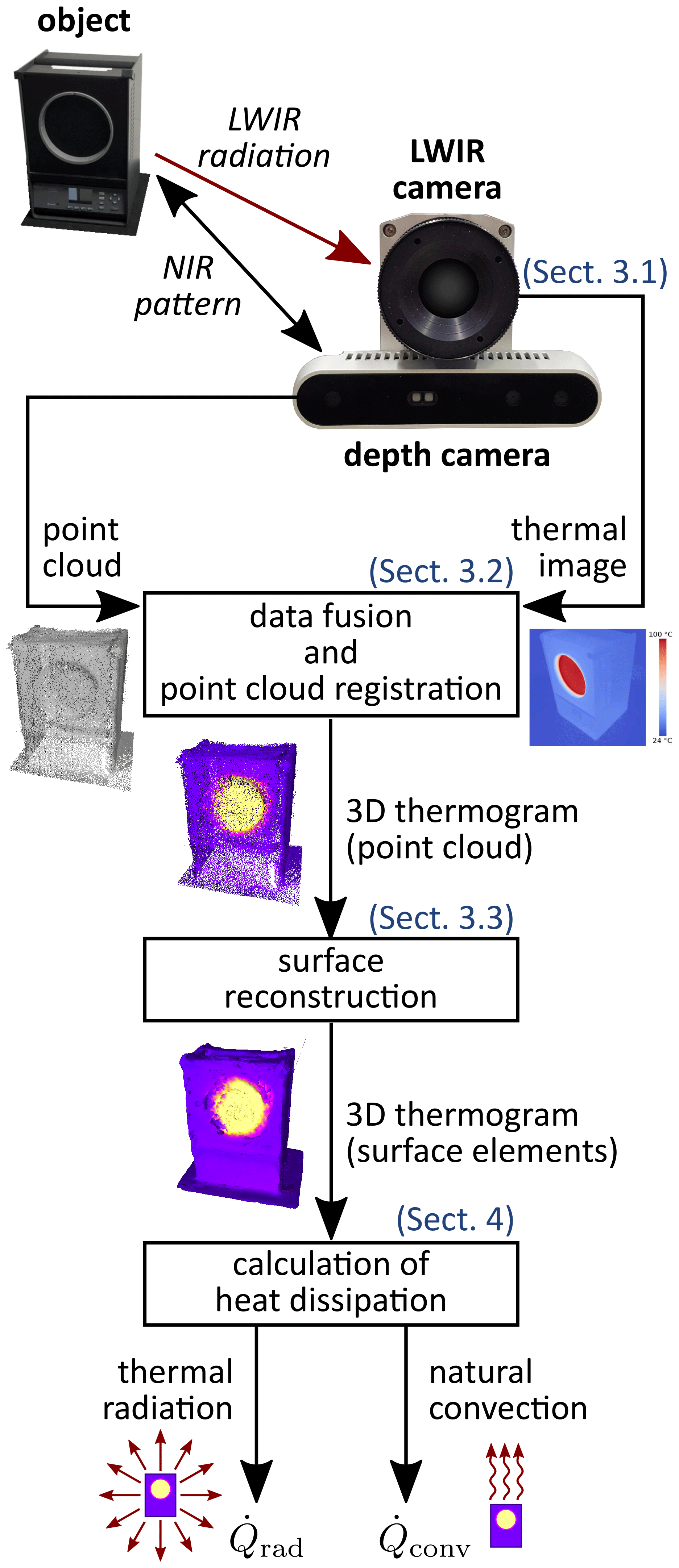
3.1 Hardware

The hardware of the measurement system consists of a long-wave infrared (LWIR) camera and a depth camera.

The LWIR camera is an Optris PI 450 with a thermal range from −20 to 100 ^∘C, a spectral range from 7.5 to 13 µm, a spatial resolution of 382 px × 288 px, a field of view of $\mathrm{53}{}^{\circ }\times \mathrm{38}{}^{\circ }$ and a frame rate of 80 Hz, see the camera datasheet (Optris, 2018) for details.

The depth camera is an Intel RealSense D415 with a depth range from 0.31 to 10 m. This device consists of one NIR projector, two NIR cameras and one visual camera. The NIR projector projects a static pattern onto the object to be measured. The scene is recorded by the two NIR cameras in a stereo setup (spectral range: 0.4 to 0.865 µm, spatial resolution: 640 px × 480 px, field of view: $\mathrm{48}{}^{\circ }\times \mathrm{40}{}^{\circ }$ and frame rate 60 Hz, see the datasheet Intel, 2020 for further information). Additionally, the visual camera records RGB images of the scene. In the RealSense D415 device the depth image calculation (stereo matching) is carried out on its internal hardware with optimized algorithms. Depth images are directly provided by the camera. In cases of highly reflective or in opposite highly absorbent surfaces it is possible that the projected pattern is not visible in the NIR stereo images and that the depth image and thus the point cloud becomes poor. This also applies for outdoor use, where the pattern is outshone by sunlight. Therefore, the depth camera is particularly useful for indoor applications and for objects up to a few meters.

3.2 Data fusion and point cloud registration

The thermal image of the LWIR camera has to be projected onto the geometric 3D data (point cloud) of the depth camera. This task is performed by a camera model with so-called intrinsic camera parameters for each involved camera and a rotation matrix and a translation vector for the relationship between the camera's coordinate systems. To calculate the parameters of these models, a geometric calibration has to be carried out once during the construction of the 3D thermography system. In this step images of a specialized calibration target (e.g. a heated chessboard with fields of different emissivity) are acquired with the assembled cameras, and the calibration parameters are calculated. For details, see Schramm et al. (2021b).

The data resulting from one single system pose does not cover the whole surface of a 3D object. At one viewing angle, the “back side” is not visible, and there may be “holes” in the 3D and thermal data caused by object occlusions. To overcome this, the object is captured from different views. For this reason, the measurement system is moved around the object to record multiple thermal point clouds resulting from different viewing angles. These point clouds have to be registered into a single overall 3D thermal model. This task is automatically done by self-localization and mapping algorithms, for details see Schramm et al. (2021a).

The measurement system is carrying out the point cloud registration and the fusion of spatial and thermal information in real-time. Therefore, the self-localization and mapping algorithms are implemented on a graphics card of a portable high-performance computer. The result of this step is a dense point cloud of the whole measurement object surface. After the data fusion with the thermal image each point of the cloud contains a value for its apparent temperature. These temperature values are coded by a color map and stored as colors. The reason is that the real-time computation of the point cloud registration and the rendering of the 3D object is optimized for using color data. In a post-processing step, the temperatures are recalculated from the color values. The result of this step is called a 3D thermogram.

3.3 Surface reconstruction

The surface reconstruction step is executed “offline”, when the complete 3D thermogram (point cloud) of the measured object is available. It is assumed that the point cloud contains only the object of interest; i.e. walls, mounting and so on are cropped due to the measuring range of the depth camera and/or manually removed in an intermediate step. The point cloud is converted into surface elements by a Poisson surface reconstruction. This is done by using the open-source library Open3D (Zhou et al., 2018). The quality of the Poisson surface reconstruction depends on the parametrization of the algorithm. Especially the octree depth (relative resolution of the surface reconstruction) should be increased with growing object complexity (which will lead to longer computation times). In this work, good results were obtained for a depth level of 13. For details, the reader is referred to Kazhdan and Hoppe (2013).

The result is a 3D thermogram consisting of triangle surface elements (exemplary shown in Fig. 2, right). In a subsequent step it is recommended to smooth the surface and to reduce the number of surface elements. This leads to a significantly reduced computing time for the calculation of the heat dissipation. A build-in function for the automatic removal of degenerated triangles is used. In a last step the triangle normals are calculated by a standard neighborhood search method. The normals are defined in the direction pointing out of the object.

Figure 2 Illustration of the differences between a point cloud (left) and a surface reconstruction (right) with the triangle net in a close-up view for the exemplary application of a silicone extrusion line infrared heater. The full 3D thermogram consists of 1 031 567 points and 2 050 545 triangles.

4 Calculation of heat dissipation

After the surface reconstruction step, the 3D thermogram consists of N triangle surface elements, each with a temperature T_i, i=1, …, N. For the temperature measurement, the object is assumed to be a gray body. The emissivity ε_i of each surface element has to be determined previously. The area A_i of each triangle surface element with side lengths a_i, b_i, and c_i can be calculated by Heron's formula:

$$\begin{array}{}\text{(1)}& A_i=\sqrt{s_{\mathrm{\Delta },i}\cdot \left(s_{\mathrm{\Delta },i}-a_i\right)\cdot \left(s_{\mathrm{\Delta },i}-b_i\right)\cdot \left(s_{\mathrm{\Delta },i}-c_i\right)},\end{array}$$

with

$$\begin{array}{}\text{(2)}& s_{\mathrm{\Delta },i}={\displaystyle \frac{\mathrm{1}}{\mathrm{2}}}\cdot \left(a_i+b_i+c_i\right).\end{array}$$

In the following, the calculation of the radiant as well as the natural convective heat dissipation of a measuring object is presented. The total heat dissipation is calculated by adding up the two components (assuming negligible forced convection and conduction).

4.1 Thermal radiation

To calculate the heat flow caused by thermal radiation ${\dot{Q}}_{\mathrm{rad}}$, the Stefan–Boltzmann law can be used (VDI, 2013):

$$\begin{array}{}\text{(3)}& {\dot{Q}}_{\mathrm{rad}}=\sum _{i=\mathrm{1}}^N{A}_i\cdot {\mathit{\epsilon }}_i\cdot \mathit{\sigma }\cdot \left(T_i^{\mathrm{4}}-T_{\mathrm{amb}}^{\mathrm{4}}\right),\end{array}$$

where σ is the Stefan–Boltzmann constant and T_amb is the ambient radiation temperature, which is assumed to be known and constant over the entire ambient (see Fig. 3, left). Finally, the heat flow due to thermal radiation of each triangle is summed up for all i=1, …, N triangle surface elements. Equation (3) assumes that border effects and mutual influences of the surface elements are neglected. This holds roughly for mainly convex objects in indoor environments, where the objects are some amount smaller than the room.

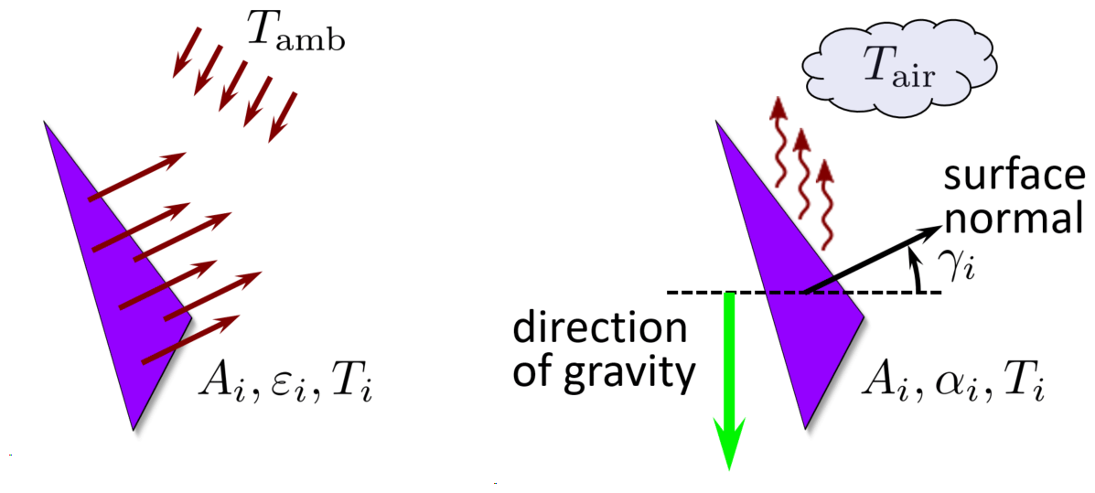
Figure 3 Sketch of the triangle with the parameters for the calculation of the heat flow caused by thermal radiation (left) and natural convection (right).

4.2 Natural convection

Since the natural convection always flows in the opposite direction to gravity, the gravity vector must be specified in the 3D thermogram. With this vector and the triangle surface normal, the altitude angle γ_i is known; see Fig. 3.

The heat flow by natural convection ${\dot{Q}}_{\mathrm{conv}}$ can be calculated by (VDI, 2013):

$$\begin{array}{}\text{(4)}& {\dot{Q}}_{\mathrm{conv}}=\sum _{i=\mathrm{1}}^N{A}_i\cdot {\mathit{\alpha }}_i\cdot \left(T_i-T_{\mathrm{air}}\right).\end{array}$$

The area A_i, the surface temperature T_i and the surrounding air temperature T_air (far away from the surface) are known. The air temperature T_air and the ambient radiation temperature T_amb (e.g. room walls/ceilings/floors) are often approximately equal. However, in thermally non-stationary rooms or for outdoor measurements, each value should be determined separately. For the determination of the heat transfer coefficient α_i empirical equations can be used (VDI, 2013):

$$\begin{array}{}\text{(5)}& {\mathit{\alpha }}_i={\displaystyle \frac{N{u}_i\cdot \mathit{\lambda }}{L_i}},\end{array}$$

with the Nusselt number Nu_i, the thermal conductivity λ of the surrounding air and the characteristic length L_i. The Nusselt number Nu_i can be determined as a function of the Rayleigh number Ra and the Prandtl number Pr. The explicit functions and values for the Nusselt, Rayleigh, and Prandtl numbers depend on

1. the driving temperature difference T_i−T_air,

2. properties of the surrounding air (coefficient of thermal expansion β, kinematic viscosity ν, and thermal diffusivity κ),

3. the characteristic length L_i,

4. the surface orientation relative to the gravity direction (the altitude angle γ_i), and

5. the acceleration of gravity g.

The properties of the surrounding air (β, ν, κ, and λ) are temperature-dependent and available in look-up tables. The values of dry air (Table 1 in Sect. D2.2 of VDI, 2013) were used for the following experiments. The calculation of the Nusselt number Nu_i is specified in chapter F2 of the latter reference.

The characteristic length L_i in Eq. (5) is defined as the area of the whole overflowed surface divided by the perimeter of the projection in the flow direction. For this reason the calculation depends on the dimension and the altitude angle γ_i of each surface element. Three cases are distinguished:

1. for vertical surfaces (γ_i=0^∘), the characteristic length is the maximal overall vertical height of the object L_i=h,

2. for horizontal surfaces (${\mathit{\gamma }}_i=\pm \mathrm{90}$^∘), the characteristic length is calculated as $L_i=\frac{w\cdot d}{\mathrm{2}(w+d)}$, with the horizontal object width w and depth d, and

3. for surfaces between γ_i=0^∘ and ${\mathit{\gamma }}_i=\pm \mathrm{90}$^∘, the L_i values are interpolated.

5 Experimental validation

For the experimental validation of the presented approach, two objects were investigated, and their heat dissipation was calculated. The first object was an infrared area calibrator (IR calibrator); see Fig. 4. The second object was an infrared radiator (IR radiator); see Figs. 5 and 6. It has to be noted that the IR calibrator was used for the parametrization of the reconstruction pipeline (see Sect. 5.1).

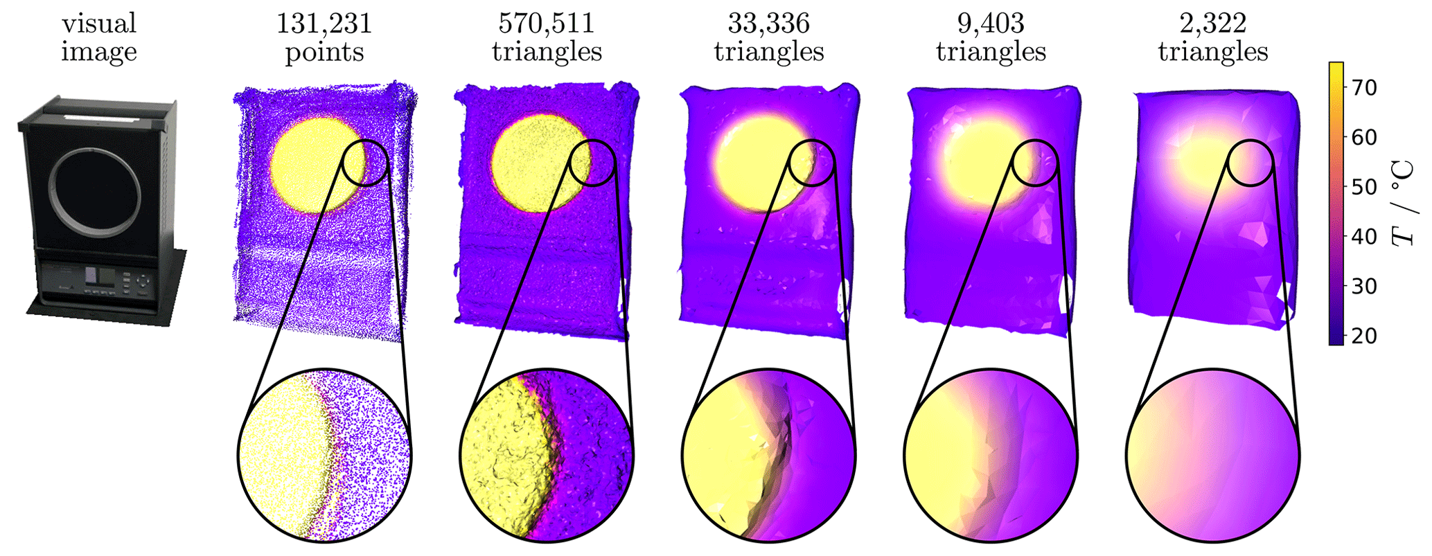
Figure 4 Visual image and different representations (point cloud and reconstructed surfaces with variable vertex reduction settings d_red) of the IR calibrator experiment 3D thermogram (rear side not shown but measured and available in 3D data).

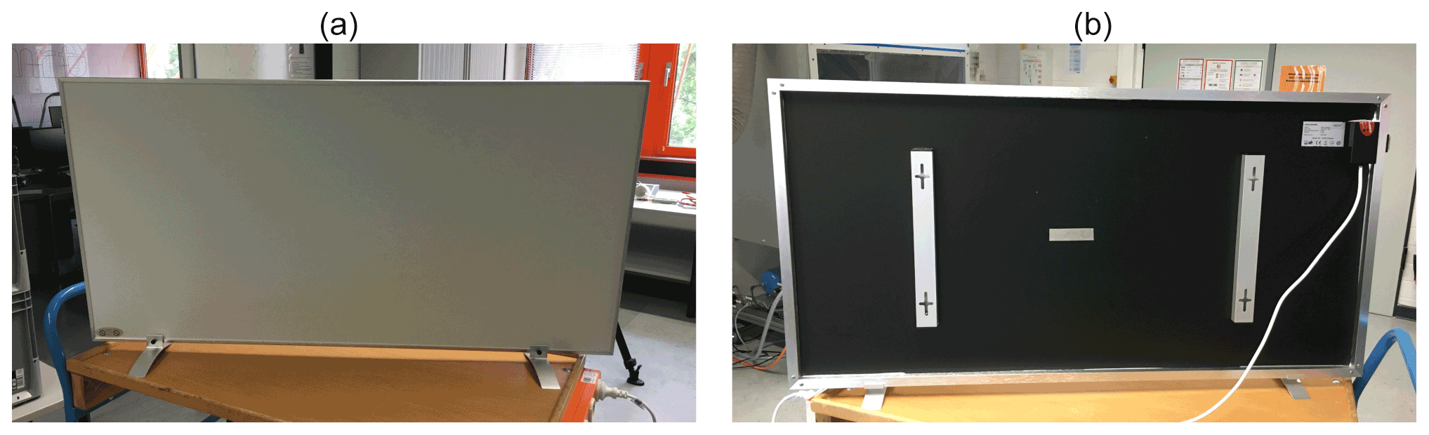
Figure 5 Visual images of the infrared radiator experiment with front (a) and rear (b) panels.

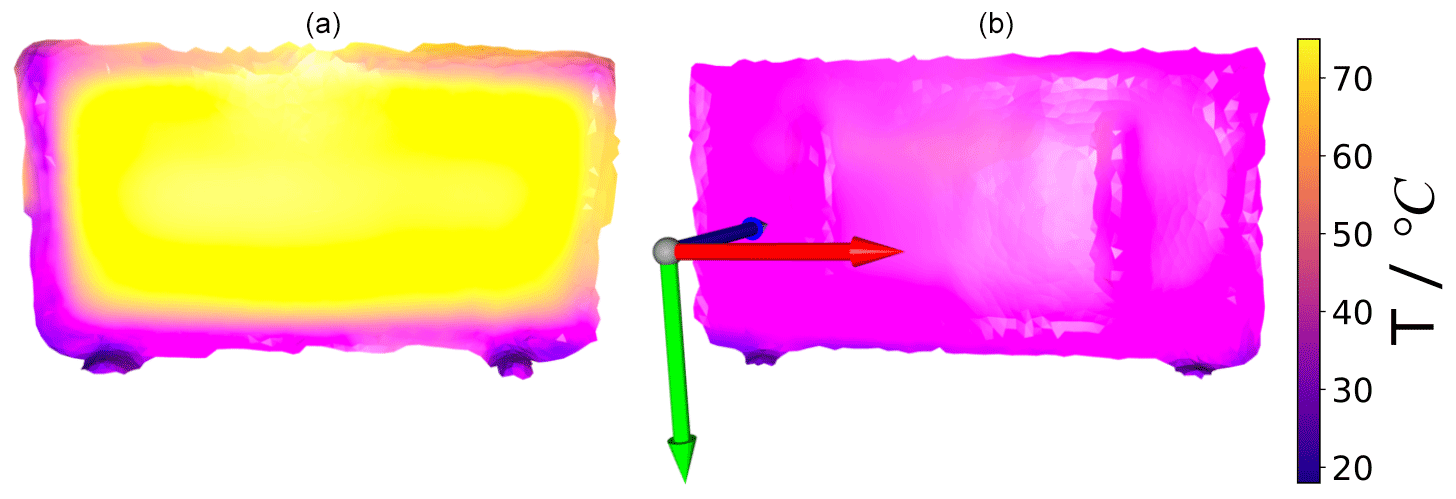
Figure 6 Front (a) and rear (b) views of a 3D thermogram (triangle surface elements) of the infrared radiator shown in Fig. 5.

The subsequent physically motivated calculations (see Sect. 4) do not have algorithmic parameters. Thus, no user choices had to be made. However, additional physical parameters had to be measured (e.g. air temperature T_air, emissivity ε). After these investigations, and having set the reduction parameter, the heat dissipation of the second object (infrared radiator) was calculated automatically without any change in the preprocessing algorithmic parameters.

5.1 Parametrization of the surface reconstruction

For the parametrization of the surface reconstruction, the parameter that determines the reduction of the triangle surface elements was investigated; see Fig. 4 and Table 1. The adjustable parameter for this algorithm was the distance threshold between vertices d_red. For smaller distances vertices are merged into one by averaging positions, surface normals, and temperature values. In Fig. 4 it can be seen that the reconstructed surfaces (which were planar) were coarse after the Poisson surface reconstruction (570 511 triangles). This was caused by the measurement noise of the depth sensor. For this reason, the reduction of the triangle surface elements had two advantages: (1) the resulting surface was smoothed and (2) the subsequent calculation time was significantly reduced. As can be seen in Fig. 4, the surface with 2322 triangles was too smooth, so that the edges are smoothed out. The surface with 33 336 triangles remains uneven. The reduction to 9403 triangles (d_red=0.01 m) was chosen as a compromise between an even surface and the remaining edges. The significant reduction of the calculation time (see Table 1) is especially useful when the method is applied to large 3D thermograms (see e.g. Fig. 2). It has to be remarked that the quality of the reconstructed surface and the required degree of reduction and smoothing strongly depend on the used 3D sensor, the measurement conditions (e.g. NIR interference radiation, reflectance of the object in NIR), and the reconstruction algorithm.

Table 1 Number of triangle surface elements of the IR calibrator 3D thermogram after the reduction using different distance parameter values in the reduction algorithm, resulting surface area of the triangles, and CPU time needed (Intel i7-7500U).

5.2 Experimental setup

To calculate the heat dissipation of the objects, at first a 3D thermogram was recorded. Attention was paid to the fact that there were no holes in the thermograms. In addition, parts of the point clouds that do not belong to the examined object were removed. The mean air temperature T_air and ambient radiation temperature T_amb were measured by an air temperature sensor and the infrared camera respectively. Both were equal to approx. 22 ^∘C. It was considered that no intense external radiation (e.g. direct sunlight) irradiated on the object. The air properties (e.g. humidity) were assumed to be similar to the values from the lookup tables of Sect. 4.2.

The IR calibrator emitted the radiation of a black body at 70 ^∘C (virtual temperature by the manufacturer's calibration), and therefore the emissivity was set to 1. Although the painted calibrator housing may have a lower emissivity, the emissivity of the calibration surface was taken as the given parameter since it had a strong influence on the result due to the higher temperature. In the case of the IR radiator, emissivities of ε≈0.95 were determined (on the front side and backside) by using a reference tape. Since both sides have a homogeneous painted surface, this value was assumed for the entire object. Generally, it is possible to assign individual emissivities for each surface element, but in our case mean emissivities were used. The apparent temperatures stored in the point cloud were corrected using the emissivity ε, the reflected ambient radiation temperature T_amb, and the calibration curve of the camera. The IR radiator was heated up until a thermal stationary state was reached. There is no closed-loop control built into the radiator, so the electrical power consumption was stationary too. In contrast, the temperature of the IR calibrator was closed-loop-controlled, but it was observed that the temperature and the power consumption were nearly stationary during the measurement.

To get a reference for the heat dissipation, the electrical power consumption was measured by a wattmeter (uncertainty $\mathit{\sigma }=\pm \mathrm{2}$ %). As a reference for the quality of the surface reconstruction, the triangle surface element areas of the 3D thermogram were summed up and compared to the surface area measured with a folding rule. The measured area by the folding rule was only determined by the main dimensions. Elevations and cavities were not included. In the case of the IR calibrator, the bottom side is not added to the area, but this is the case for the folding rule measurement and the 3D thermogram.

5.3 Results and discussion

The recordings were processed according to the methods outlined in Sect. 4. The resulting number of measurement points and surface elements for each experiment are shown in Table 2.

Table 2 Number of points and triangle surface elements of the 3D thermograms after the performed experiments and processing steps.

The measurement results for the surface area, the heat dissipation, and the corresponding references are presented in Table 3. The average heat transfer coefficient was ${\stackrel{\mathrm{‾}}{\mathit{\alpha }}}_{\mathrm{cal}}=\mathrm{2.67}$ W m⁻² K⁻¹ for the calibrator and ${\stackrel{\mathrm{‾}}{\mathit{\alpha }}}_{\mathrm{rad}}=\mathrm{4.30}$ W m⁻² K⁻¹ for the radiator. Despite the fact that the folding rule measurement of the area is approximate, it can be assumed that the surface areas were slightly overestimated for both objects. A look into the details shows that the measured front area of the infrared radiator was bigger than the rear area. That is not true for this object. Figure 6 indicates that the surface of the infrared radiator was reconstructed with a remaining uneven surface (visible at the edges). The unevenness was even stronger in case of the reconstructed surface, with neither smoothing nor reduction of surface elements (comparable to the IR calibrator in Fig. 4). Here a more precise 3D sensor or an improved surface reconstruction (parameters and/or algorithms) could improve the results by either having less noisy data or by filtering them directly during the registration. For example, the point cloud could be segmented into larger simple geometries (e.g. planes, cubes, cylinders), which could then be used for the computation instead of the noisy point cloud data.

Table 3 Calculated surface area and heat dissipation of the infrared calibrator and the radiator. As a reference the area (measured with a folding rule) and the electrical power consumption (measured by a wattmeter) are given. ^* The overall heat dissipation is the sum of radiation and convection, but the values have more decimal places and are rounded in the table.

The heat dissipation was significantly underestimated for the calibrator and moderately overestimated for the radiator (see Table 3). In the case of the calibrator, this results from the integrated cooling slits and an active fan cooling on the backside, which caused forced convection that is not measurable by the system. The corresponding air flows were not covered by the model. In the radiator's case, these potential sources of error were not present, and the results were closer to the reference. Heat conduction to the floor space should be negligible due to the low bottom temperature of the IR calibrator and the small contact area of the radiator. The total area of the radiator was overestimated by 4.76 %. This was mainly due to the remaining noise in the reconstructed surface. The heat loss was overestimated by 7.60 %, which was largely caused by the surface area uncertainty. The remaining uncertainty can have various reasons, such as the uncertainty of the infrared camera measurements or the accuracy of the physical parameters determined before the measurement (e.g. ambient temperature, emissivity).

A detailed uncertainty analysis has not been carried out yet. Due to the large number of potential influencing factors (e.g. ambient temperature, emissivity, thermal and spatial camera uncertainty, geometrical and temporal camera calibration, model assumptions), an estimation based on the propagation of uncertainty does not seem to be appropriate. A statement about the repeatability should be made with multiple measurements and the determination of the results' standard deviation in the future. Due to this missing step, no statements about the uncertainty are given in this paper.

6 Conclusions

In this work, the information of a 3D thermogram is used to calculate the heat dissipation of the measured objects. For this purpose, the surface of the 3D temperature point cloud is reconstructed. Using the calculated surface area and the measured temperatures, the natural convection and the radiant power of the measurement object can be determined. As additional information, only the emissivities of the surfaces, the ambient radiation temperature and the air temperature must be known or measured. Uncertainties appear especially in the case of inhomogeneous objects, where the emissivity is determined at only one or a few points. Due to the measurement process, the objects must be quasistatic in position and temperature. Additionally, the depth camera is limited in resolving small structures such as cooling fins. Internal heat flows, forced convection (e.g. due to a cooling fan) or the use of e.g. slits in the surface could not be covered by the measuring system, which is apparent in the results of the calibrator case study. In summary, the presented sensor system and data evaluation method enable the direct measurement of the surface heat dissipation by thermal radiation and natural convection, e.g. to calculate losses and to optimize the efficiency of technical systems.

Future work may address an improved surface reconstruction, e.g. by a better smoothing and/or outlier removal. Up to now, no mutual influence of the triangle surface elements has been considered. If this is known, forced convection could be taken into account. Instead of the semi-empirical equations, especially for the convection, this could be done by using computational fluid dynamics. Newer algorithms for point cloud registration, see Schramm et al. (2021a), can generate 3D thermograms of larger objects. Finally, an uncertainty analysis should be performed, and the system should be tested in industrial use cases (e.g. hardening furnaces or other heat-carrying machines and plants; see Schramm et al., 2021a, for examples).