Influence of measurement uncertainty on machine learning results demonstrated for a smart gas sensor

Humans spend most of their lives indoors, so indoor air quality (IAQ) plays a key role in human health. Thus, human health is seriously threatened by indoor air pollution, which leads to 3.8 ×10⁶ deaths annually, according to the World Health Organization (WHO). With the ongoing improvement in life quality, IAQ monitoring has become an important concern for researchers. However, in machine learning (ML), measurement uncertainty, which is critical in hazardous gas detection, is usually only estimated using cross-validation and is not directly addressed, and this will be the main focus of this paper. Gas concentration can be determined by using gas sensors in temperature-cycled operation (TCO) and ML on the measured logarithmic resistance of the sensor. This contribution focuses on formaldehyde as one of the most relevant carcinogenic gases indoors and on the sum of volatile organic compounds (VOCs), i.e., acetone, ethanol, formaldehyde, and toluene, measured in the data set as an indicator for IAQ. As gas concentrations are continuous quantities, regression must be used. Thus, a previously published uncertainty-aware automated ML toolbox (UA-AMLT) for classification is extended for regression by introducing an uncertainty-aware partial least squares regression (PLSR) algorithm. The uncertainty propagation of the UA-AMLT is based on the principles described in the Guide to the Expression of Uncertainty in Measurement (GUM) and its supplements. Two different use cases are considered for investigating the influence on ML results in this contribution, namely model training with raw data and with data that are manipulated by adding artificially generated white Gaussian or uniform noise to simulate increased data uncertainty, respectively. One of the benefits of this approach is to obtain a better understanding of where the overall system should be improved. This can be achieved by either improving the trained ML model or using a sensor with higher precision. Finally, an increase in robustness against random noise by training a model with noisy data is demonstrated.

1 Introduction

1.1 Indoor air quality and VOCs

As humans spend most of their lives indoors, the most significant environment for them is the indoor environment (Brasche and Bischof, 2005). For this reason, indoor air quality (IAQ) is of special importance as it plays a leading role with regard to the performance, well-being, and health of humans (Sundell, 2004; Asikainen et al., 2016). Volatile organic compounds (VOCs) are one of the main contributors to poor air quality, especially in indoor air, and can lead to serious health problems, e.g., leukemia, cancers, or tumors (Jones, 1999; Tsai, 2019). Nowadays, IAQ monitoring is mostly based on measurements of carbon dioxide (CO₂) emitted by humans as the primary indicator for poor indoor air, as CO₂ concentration is directly related to VOCs caused by human presence (Von Pettenkofer, 1858). However, this neglects the fact that not only humans emit VOCs but also their activities such as household cleaning, cooking, and smoking, as well as, for example, furniture, carpets, and even the building itself due to the building materials used (Spaul, 1994). To measure almost all types of VOCs in indoor air, metal oxide semiconductor (MOS) gas sensors are widely used as they are low-cost, robust, and highly sensitive. To improve the limited selectivity of these sensors and enable the discrimination of specific pollutants, MOS gas sensors can be operated in dynamic modes, especially by using a temperature-cycled operation (TCO; Eicker, 1977; Lee and Reedy, 1999; Baur et al., 2015; Schütze and Sauerwald, 2020a; Baur et al., 2021). A TCO, especially in combination with modern microstructured gas sensors, yields extensive and rich response patterns that need to be interpreted using machine learning (ML) to extract the relevant information (Schütze and Sauerwald, 2020a).

For the data set used in this contribution, sensor responses of an SPG30 sensor (Sensirion AG, Stäfa, Switzerland) with four gas-sensitive layers in TCO were recorded (Rüffer et al., 2018). This contribution focuses on formaldehyde as an example of a highly relevant toxic gas and on the sum concentration of all VOCs (VOC_sum) in parts per billion (ppb) in the used data set, i.e., the sum of the concentrations of acetone, ethanol, formaldehyde, and toluene. VOC_sum should not be confused with the widely used total VOC (TVOC) value, as this is based on analytical measurements and takes into account only VOCs with medium volatility (Schütze and Sauerwald, 2020b). Formaldehyde (CH₂O) is one of the most toxic and carcinogenic gases in indoor air (Hauptmann et al., 2004; Zhang, 2018; NTP, 2021) and is released from a variety of sources. The most significant ones are pressed wood products, e.g., particle board and plywood paneling. The World Health Organization (WHO) set the guideline threshold for a 30 min average concentration to 0.1 mg m⁻³, which corresponds to approximately 80.1 ppb for 760 mmHg and 20 ^∘C (World Health Organization, 2010).

1.2 Automated ML toolbox

In recent years, an automated machine learning toolbox (AMLT) was developed and applied to different classification tasks (Schneider et al., 2017, 2018; Dorst et al., 2021). Its extension to an uncertainty-aware AMLT (UA-AMLT) for classification was presented in Dorst et al. (2022). As gas concentrations are continuous quantities, regression must be used, which is a supervised ML technique. In this contribution, the AMLT is therefore extended to be applicable for regression tasks and, furthermore, the corresponding uncertainty for the ML result is considered. The uncertainty propagation is based on the Guide to the Expression of Uncertainty in Measurement (GUM; BIPM et al., 2008a) and its Supplement 1 (BIPM et al., 2008b) and Supplement 2 (BIPM et al., 2011). These three documents establish general rules for evaluating and expressing measurement uncertainty. These rules and principles are applied in this contribution for estimating the uncertainty of an ML model prediction, thus extending the GUM approach to smart sensors.

To investigate the influence of measurement uncertainty on machine learning (ML) results, sensor raw data are manipulated by simulated additive white Gaussian noise. With these manipulated data sets, different ML models are determined based on feature extraction, feature selection followed by regression, and the influence of the Gaussian noise, which simulates increased sensor uncertainty in the ML results, is investigated. Gaussian (normally distributed) noise is a very good assumption for any process for which the central limit theorem holds. In addition, the influence of additive white uniform noise as a further noise model is investigated.

2 Materials and methods

2.1 Data set

A data set published in Baur et al. (2021) is used to investigate the influence of measurement uncertainty on ML results. It consists of different calibration and field test measurements of gas mixtures with the MOS gas sensor SGP30 (Sensirion AG, 2020). The gas mixtures are composed of random mixtures of seven different gases that are relevant for indoor air quality. Various VOCs, i.e., acetone, ethanol, formaldehyde, and toluene, are used together with water vapor and inorganic background gases, i.e., hydrogen and carbon monoxide, as shown in Fig. 1. The gas concentrations are mixed using Latin hypercube sampling (LHS; McKay et al., 1979) to obtain unique gas mixtures (UGMs). In this contribution, only data from the initial calibration are used. The concentration ranges for all gases during the initial calibration are shown in Table 1.

Figure 1 Gas composition for calibration consisting of random mixtures of VOCs (blue) and background gases (red; adapted from Baur et al., 2021).

Table 1 Concentration ranges for all gases during the initial calibration phase (Amann et al., 2021b).

RH is the relative humidity.

The SGP30 sensor, with its four different gas-sensitive layers, is used in TCO to improve its selectivity, sensitivity, and stability (Schultealbert et al., 2018). As shown in Fig. 2, the temperature cycle consists of 10 steps at 400 ^∘C, with a duration of 5 s each, followed by different low-temperature steps, with a duration of 7 s each. One single temperature cycle thus lasts 120 s and, due to the sampling rate of 20 Hz, consists of 2.400 measurement values for each gas-sensitive layer. The sensor output represents the logarithmic resistance shown for one cycle and one gas-sensitive layer in Fig. 2.

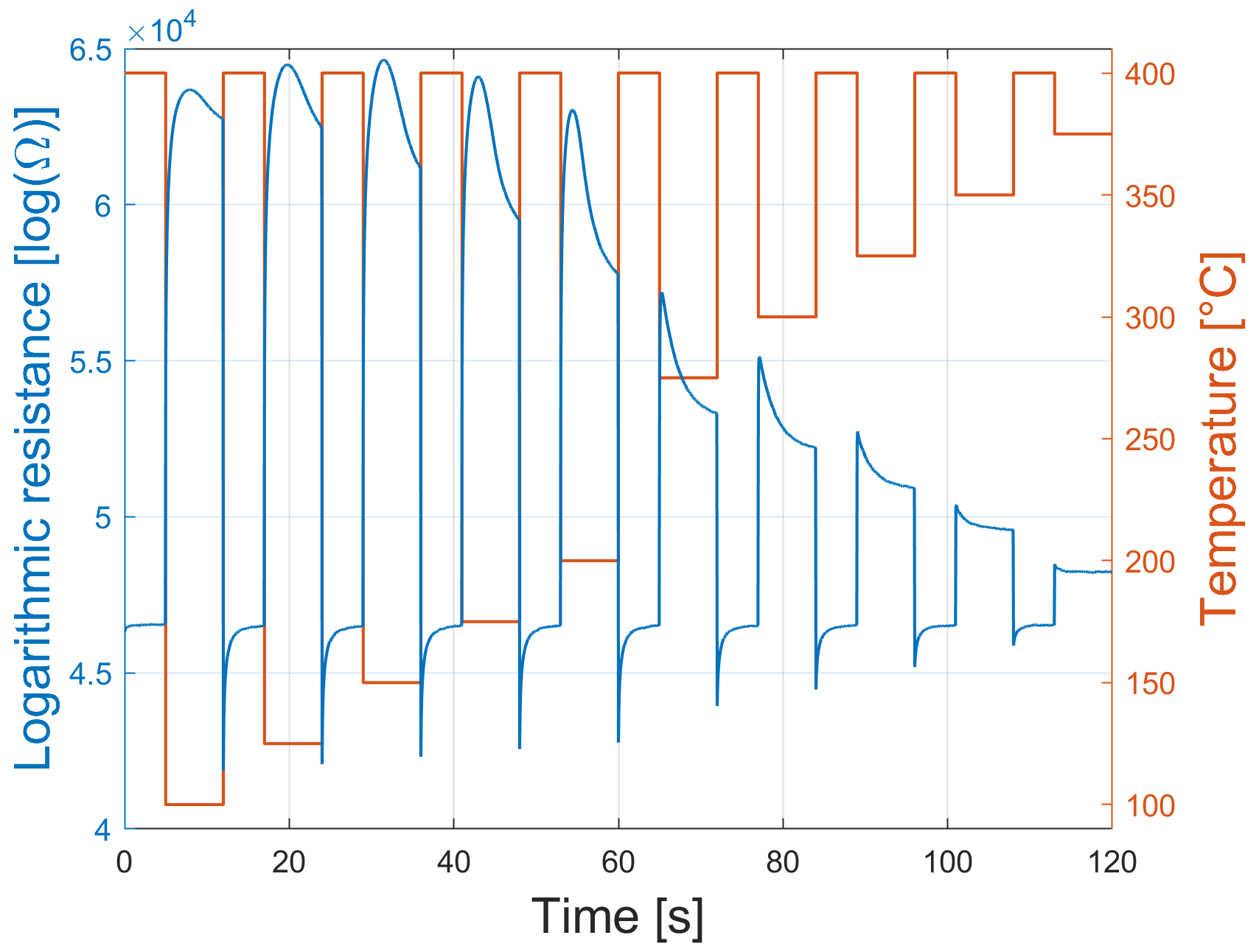
Figure 2 Logarithmic conductance of one sensor element (blue) and the temperature-cycled operation of the SGP30 (red).

During the initial calibration phase, the SGP30 sensor is exposed to 500 UGMs for 10 temperature cycles (TCs) each. Due to the limited time response of the gas mixing apparatus (GMA) and synchronization problems between sensor and GMA, four TCs at the beginning and the last TC for each UGM are omitted so that only five TCs per UGM are evaluated. Furthermore, the first three UGMs are also not considered due to run-in effects. Thus, the data set comprises 2485 relevant cycles of 497 UGMs with stable gas concentrations from the initial calibration.

2.2 Uncertainty-aware automated machine learning toolbox

In general, regression is used for predicting a continuous quantity, whereas classification is used for predicting a discrete class label. As a basis for this publication, the AMLT for classification tasks (Schneider et al., 2017, 2018; Dorst et al., 2021) and its extended uncertainty-aware version (Dorst et al., 2022) are modified to also solve regression tasks. With the AMLT, feature extraction (FE) and feature selection (FS), as well as classification/regression and evaluation, are performed without expert knowledge and without a detailed physical model of the process to minimize model generation costs. Model training, in addition to application, can be carried out with the (uncertainty-aware) AMLT. Partial least squares regression (PLSR) as the de facto standard for quantification in the field of gas sensors (Wold et al., 2001; Gutierrez-Osuna, 2002) is used for regression tasks in the AMLT. Another well-known regression algorithm is principal component regression (PCR), which first performs the principal component analysis (PCA) as an unsupervised technique to obtain the principal components (PCs) and then uses these PCs to build the regression model. As a two-step model-building algorithm, the PCR makes interpreting the ML results harder in contrast to PLSR, which only has one step (Ergon, 2014). Using PCA leads to a relevant drawback of the PCR algorithm, as performing an unsupervised technique does not guarantee that the selected principal components for the regression model building are associated with the target. An advantage of PLSR is that it often has fewer components than PCR to achieve the same prediction level (De Jong, 1993a).

As shown in Fig. 3, five complementary FE algorithms are used within the AMLT, together with Pearson correlation for FS and PLSR, as the regression algorithm.

Figure 3 Feature extraction (red), feature selection (green), and regression (blue) algorithms of the uncertainty-aware AMLT for regression tasks.

Adaptive linear approximation splits cycles into approximately linear segments, and for each segment, the mean value and slope are extracted as features from the time domain (Olszewski et al., 2001). The best Daubechies wavelets algorithm performs a wavelet transform using a Daubechies D4 wavelet (Daubechies, 1992) to extract 10 % of the wavelet coefficients with the highest average absolute value over all cycles as features from the time frequency domain. The best Fourier coefficients algorithm performs a Fourier transform, and 10 % of the amplitudes with the highest average absolute value over all cycles and their corresponding phases are extracted from frequency domain (Mörchen, 2003). Using principal component analysis, projections on the principal components are determined (Pearson, 1901; Jackson, 1991) and used as features from the time domain. Moreover, the statistical distribution of the measurement values also includes information in the time domain (Martin and Honarvar, 1995). Thus, the cycles are split into 10 approximately equally sized segments, and the four statistical moments (mean, standard deviation, skewness, and kurtosis) are extracted for each segment as features. These five FE algorithms and the Pearson correlation as FS lead to five different algorithm combinations, each benchmarked to choose the best one for the respective application. The best combination is determined by the smallest cross-validated root mean square error (RMSE), which is a measure for the differences between the predicted y_pred∈ℝ^m and the observed target values y of the same dimension, i.e.,

$$\begin{array}{}\text{(1)}& \text{RMSE}({\mathit{y}}_{\mathbf{pred}}\mathbf{,}\mathit{y})=\sqrt{{\displaystyle \frac{\mathrm{1}}{m}}\sum _{i=\mathrm{1}}^m(y_{{\text{pred}}_i}-y_i{)}^{\mathrm{2}}}.\end{array}$$

The cross-validation (CV) scenario used is explained in Sect. 2.2.1. In general, different metrics can be used to describe the performance of a regression model; however, RMSE is one of the best interpretable error measures as it has the same unit as the prediction of the model and is also comparable to the (standard) measurement uncertainty used in describing data quality in measurement.

To use the UA-AMLT, a data matrix $\mathbf{D}\in {\mathbb{R}}^{m\times n}$ for each sensor (or sensor layer) must be given, where m denotes the number of cycles of length n. In case of non-cyclic sensor data, data must be windowed to obtain the correct m×n format. Furthermore, there must be knowledge about the uncertainty matrix $\mathbf{U}\in {\mathbb{R}}^{m\times n}$, which assigns an uncertainty value u_ij to a measurement value $d_{ij}\forall i,j$. This means that correlation of errors at different time instants is neglected.

Uncertainty-aware feature extraction and selection

To perform FE, which mathematically describes the mapping D↦F_E, five complementary methods are used. In this step, one feature matrix ${\mathbf{F}}_{\mathbf{E}}\in {\mathbb{R}}^{m\times k}$, k≤ n is calculated for each of the FE methods. The uncertainty calculation is performed according to Dorst et al. (2022), so that, for every feature matrix F_E, an uncertainty matrix ${\mathbf{U}}_{{\mathbf{F}}_{\mathbf{E}}}$ of the same dimension is calculated.

In the uncertainty-aware FS step, features are ranked according to their weighted Pearson correlation to the target value, i.e., in this contribution to the gas concentration. In weighted Pearson correlation, the reciprocals of the squared uncertainty values of the features are used as weights (Dorst et al., 2022). After ranking the features, a 10-fold stratified CV (Kohavi, 1995) is carried out for every possible number of features, and the minimum CV error is determined based on the optimal number of features l∈ℕ found. From a mathematical point of view, FS is a mapping F_E↦F_S, with ${\mathbf{F}}_{\mathbf{S}}\in {\mathbb{R}}^{m\times l}$, l<k containing only the optimal number of the most relevant features according to weighted Pearson correlation. The corresponding uncertainty matrix is ${\mathbf{U}}_{{\mathbf{F}}_{\mathbf{S}}}\in {\mathbb{R}}^{m\times l}$.

2.3 Partial least squares regression

Let a predictor matrix $\mathbf{X}\in {\mathbb{R}}^{m\times l}$ and a responses matrix $\mathbf{Y}\in {\mathbb{R}}^{m\times s}$ be given. The basic algorithm for computing a PLSR of Y on X using n_comp PLSR components is developed in Wold et al. (1984). Performing PLSR means iteratively solving the following decompositions, such that the covariance between X and Y is maximized as follows:

$$\begin{array}{}\text{(2)}& {\displaystyle }\mathbf{X}={\mathbf{X}}_{\mathbf{S}}\cdot {{\mathbf{X}}_{\mathbf{L}}}^{\top }+{\mathbf{X}}_{\mathrm{res}}\text{(3)}& {\displaystyle }\mathbf{Y}={\mathbf{Y}}_{\mathbf{S}}\cdot {{\mathbf{Y}}_{\mathbf{L}}}^{\top }+{\mathbf{Y}}_{\mathrm{res}},\end{array}$$

where ${\mathbf{X}}_{\mathbf{L}}\in {\mathbb{R}}^{l\times n_{\mathrm{comp}}}$ and ${\mathbf{Y}}_{\mathbf{L}}\in {\mathbb{R}}^{s\times n_{\mathrm{comp}}}$ denote the orthogonal loading matrices. ${\mathbf{X}}_{\mathbf{S}}\in {\mathbb{R}}^{m\times n_{\mathrm{comp}}}$ and ${\mathbf{Y}}_{\mathbf{S}}\in {\mathbb{R}}^{m\times n_{\mathrm{comp}}}$ are the predictor and response scores, respectively. The matrices X_res and Y_res are the residual terms for predictor and response, respectively, and are used as a start for the next iteration step.

In MATLAB^®, the partial least squares regression (PLSR) is calculated using the SIMPLS (statistically inspired modification of the partial least squares) algorithm (De Jong, 1993b). The advantage of SIMPLS is that the regression coefficients are determined directly without inverse matrices or singular value decomposition. Assume that $\widehat{\mathbf{X}}\in {\mathbb{R}}^{m\times (l+\mathrm{1})}$ denotes a matrix in which a vector of ones is prepended to X to compute coefficient estimates for a model with constant terms. With 𝟙∈ℝ^m denoting a vector containing only ones, it holds for the augmented matrix that $\widehat{\mathbf{X}}=\left(\text{𝟙}|\mathbf{X}\right)\in {\mathbb{R}}^{m\times (l+\mathrm{1})}$. The SIMPLS algorithm involves the calculation of a weighted matrix $\mathbf{W}\in {\mathbb{R}}^{(l+\mathrm{1})\times n_{\mathrm{comp}}}$. For the SIMPLS algorithm, the following holds:

$$\begin{array}{}\text{(4)}& {\displaystyle }{\mathbf{X}}_{\mathbf{S}}=\widehat{\mathbf{X}}\cdot \mathbf{W}\text{and}\text{(5)}& {\displaystyle }\mathbf{Y}={\mathbf{X}}_{\mathbf{S}}\cdot {{\mathbf{Y}}_{\mathbf{L}}}^{\top }.\end{array}$$

Combining Eqs. (4) and (5) leads to the following:

$$\begin{array}{}\text{(6)}& {\displaystyle }\mathbf{Y}=\widehat{\mathbf{X}}\cdot \mathbf{W}\cdot {{\mathbf{Y}}_{\mathbf{L}}}^{\top }\text{(7)}& {\displaystyle }=\widehat{\mathbf{X}}\cdot \mathbf{B},\end{array}$$

where $\mathbf{B}\in {\mathbb{R}}^{(l+\mathrm{1})\times s}$ denotes the matrix containing intercept terms in the first row and PLSR coefficient estimates in the others (De Jong, 1993b).

Uncertainty-aware partial least squares regression

In this contribution, the target values y∈ℝ^m are only represented by one vector, which leads to the matrix B (see Sect. 2.3) being also only a vector $\mathit{\beta }\in {\mathbb{R}}^{l+\mathrm{1}}$. The matrix of selected features is given by ${\mathbf{F}}_{\mathbf{S}}\in {\mathbb{R}}^{m\times l}$. ${\widehat{\mathbf{F}}}_{\mathbf{S}}=\left(\text{𝟙}|{\mathbf{F}}_{\mathbf{S}}\right)\in {\mathbb{R}}^{m\times (l+\mathrm{1})}$ denotes the matrix where one column of ones at the beginning of F_S was added. For PLSR, the following holds:

$$\begin{array}{}\text{(8)}& {\mathit{y}}_{\mathbf{pred}}={\widehat{\mathbf{F}}}_{\mathbf{S}}\cdot \mathit{\beta },\end{array}$$

with y_pred∈ℝ^m representing the predicted target values. The basis of the uncertainty values calculation for the prediction y_pred are formulas given in Sect. 6.2 (“Propagation of uncertainty for explicit multivariate measurement models”) found in Supplement 2 of GUM (GUMS2; BIPM et al., 2011). This section of GUMS2 shows the covariance matrix calculation associated with an estimate of a multidimensional output quantity with the help of a sensitivity matrix using matrix–vector notation. This approach can be transferred to the propagation of uncertainty for PLSR. The first step is the transposing of Eq. (8), which leads to the following:

$$\begin{array}{}\text{(9)}& {\mathit{y}}_{\mathbf{pred}}^{\top }={\mathit{\beta }}^{\top }\cdot {\widehat{\mathbf{F}}}_{\mathbf{S}}^{\top }.\end{array}$$

To use Sect. 6.2 of GUMS2, ${\widehat{\mathbf{F}}}_{\mathbf{S}}$ and β must be transformed into vector and matrix, respectively. For the columns of ${\widehat{\mathbf{F}}}_{\mathbf{S}}^{\top }$, the following holds:

$$\begin{array}{}\text{(10)}& {\widehat{\mathbf{F}}}_{\mathbf{S}}^{\top }=\left(\begin{array}{cccc}& \mathrm{1}& \mathrm{\dots }& \mathrm{1}\\ {\mathit{f}}_{{\mathit{S}}_{\mathbf{1}}}^{\top }& {\mathit{f}}_{{\mathit{S}}_{\mathbf{2}}}^{\top }& \mathrm{\dots }& {\mathit{f}}_{{\mathit{S}}_{\mathit{m}}}^{\top }\end{array}\right),\end{array}$$

where ${\mathit{f}}_{{\mathit{S}}_{\mathit{i}}}^{\top }\in {\mathbb{R}}^l$, $\forall i=\mathrm{1},\mathrm{\dots },m$ denotes the selected features for the ith cycle. Thus, the matrix–vector representation is given by the following:

$$\begin{array}{}\text{(11)}& {\stackrel{\mathrm{̃}}{\mathit{F}}}_{\mathit{S}}^{\top }=\left(\begin{array}{c}\mathrm{1}\\ {\mathit{f}}_{{\mathit{S}}_{\mathbf{1}}}^{\top }\\ \mathrm{1}\\ {\mathit{f}}_{{\mathit{S}}_{\mathbf{2}}}^{\top }\\ \mathrm{⋮}\\ \mathrm{1}\\ {\mathit{f}}_{{\mathit{S}}_{\mathit{l}}}^{\top }\end{array}\right)\in {\mathbb{R}}^{(m\cdot (l+\mathrm{1}\left)\right)\times \mathrm{1}},\end{array}$$

and ${\stackrel{\mathrm{̃}}{\mathit{\beta }}}^{\top }\in {\mathbb{R}}^{m\times (m\cdot (l+\mathrm{1}\left)\right)}$, with

$$\begin{array}{}\text{(12)}& {\stackrel{\mathrm{̃}}{\mathit{\beta }}}^{\top }=\left(\begin{array}{ccccc}{\mathit{\beta }}^{\top }& \mathrm{0}\mathrm{\dots }\mathrm{0}& \mathrm{0}\mathrm{\dots }\mathrm{0}& \mathrm{\dots }& \mathrm{0}\mathrm{\dots }\mathrm{0}\\ \mathrm{0}\mathrm{\dots }\mathrm{0}& {\mathit{\beta }}^{\top }& \mathrm{0}\mathrm{\dots }\mathrm{0}& \mathrm{\dots }& \mathrm{0}\mathrm{\dots }\mathrm{0}\\ \mathrm{0}\mathrm{\dots }\mathrm{0}& \mathrm{0}\mathrm{\dots }\mathrm{0}& {\mathit{\beta }}^{\top }& \mathrm{\dots }& \mathrm{0}\mathrm{\dots }\mathrm{0}\\ \mathrm{⋮}& \mathrm{⋮}& \mathrm{⋮}& \mathrm{\ddots }& \mathrm{⋮}\\ \mathrm{0}\mathrm{\dots }\mathrm{0}& \mathrm{0}\mathrm{\dots }\mathrm{0}& \mathrm{0}\mathrm{\dots }\mathrm{0}& \mathrm{\dots }& {\mathit{\beta }}^{\top }\end{array}\right),\end{array}$$

which leads to

$$\begin{array}{}\text{(13)}& {\mathit{y}}_{\mathbf{pred}}^{\top }={\stackrel{\mathrm{̃}}{\mathit{\beta }}}^{\top }\cdot {\stackrel{\mathrm{̃}}{\mathit{F}}}_{\mathit{S}}^{\top }.\end{array}$$

To propagate the uncertainty in the PLSR, the uncertainty matrix of the selected features ${\mathbf{U}}_{{\mathbf{F}}_{\mathbf{S}}}\in {\mathbb{R}}^{m\times l}$ must be extended with a column associated with the first column of ${\widehat{\mathbf{F}}}_{\mathbf{S}}$. Thus, it holds that ${\widehat{\mathbf{U}}}_{{\mathbf{F}}_{\mathbf{S}}}=\left(\textcolor{red}{}|{\mathbf{U}}_{{\mathbf{F}}_{\mathbf{S}}}\right)\in {\mathbb{R}}^{m\times (l+\mathrm{1})}$. The transpose matrix ${\widehat{\mathbf{U}}}_{{\mathbf{F}}_{\mathbf{S}}}^{\top }$ is transferred to the diagonal matrix ${\stackrel{\mathrm{̃}}{\mathbf{U}}}_{{\mathbf{F}}_{\mathbf{S}}}^{\top }\in {\mathbb{R}}^{(m\cdot (l+\mathrm{1}\left)\right)\times (m\cdot (l+\mathrm{1}\left)\right)}$, where the rows of ${\widehat{\mathbf{U}}}_{{\mathbf{F}}_{\mathbf{S}}}$ are in the diagonal. Using Sect. 6.2.1.3 of BIPM et al. (2011) leads to the following:

$$\begin{array}{}\text{(14)}& {\displaystyle }\stackrel{\mathrm{̃}}{\mathbf{U}}={\stackrel{\mathrm{̃}}{\mathit{\beta }}}^{\top }\cdot {\left({\stackrel{\mathrm{̃}}{\mathbf{U}}}_{{\mathbf{F}}_{\mathbf{S}}}^{\top }\right)}^{\mathrm{2}}\cdot {\left({\stackrel{\mathrm{̃}}{\mathit{\beta }}}^{\top }\right)}^{\top }\text{(15)}& {\displaystyle }={\stackrel{\mathrm{̃}}{\mathit{\beta }}}^{\top }\cdot {\left({\stackrel{\mathrm{̃}}{\mathbf{U}}}_{{\mathbf{F}}_{\mathbf{S}}}^{\top }\right)}^{\mathrm{2}}\cdot \stackrel{\mathrm{̃}}{\mathit{\beta }},\end{array}$$

with $\stackrel{\mathrm{̃}}{\mathbf{U}}\in {\mathbb{R}}^{m\times m}$. To obtain the diagonal elements of $\stackrel{\mathrm{̃}}{\mathbf{U}}$, Eq. (15) can be simplified and retransformed to the following:

$$\begin{array}{}\text{(16)}& {\displaystyle }{\mathbf{U}}_{\mathrm{PLSR}}^{\top }=\left({\mathit{\beta }}^{\top }\circ {\mathit{\beta }}^{\top }\right)\cdot \left({\widehat{\mathbf{U}}}_{{\mathbf{F}}_{\mathbf{S}}}^{\top }\circ {\widehat{\mathbf{U}}}_{{\mathbf{F}}_{\mathbf{S}}}^{\top }\right)\text{(17)}& {\displaystyle }\iff {\mathbf{U}}_{\mathrm{PLSR}}=\left({\widehat{\mathbf{U}}}_{{\mathbf{F}}_{\mathbf{S}}}\circ {\widehat{\mathbf{U}}}_{{\mathbf{F}}_{\mathbf{S}}}\right)\cdot \left(\mathit{\beta }\circ \mathit{\beta }\right)\text{(18)}& {\displaystyle }={\widehat{\mathbf{U}}}_{{\mathbf{F}}_{\mathbf{S}}}^{\circ \mathrm{2}}\cdot {\mathit{\beta }}^{\circ \mathrm{2}},\end{array}$$

where ∘ denotes the Hadamard (element-wise) product (Horn, 1990). The uncertainty values associated with y_pred can be calculated by the following:

$$\begin{array}{}\text{(19)}& {\mathit{U}}_{{\mathit{y}}_{\mathbf{pred}}}={\left(\left|{\widehat{\mathbf{U}}}_{{\mathbf{F}}_{\mathbf{S}}}^{\circ \mathrm{2}}\cdot {\mathit{\beta }}^{\circ \mathrm{2}}\right|\right)}^{\circ \mathrm{1}/\mathrm{2}}\in {\mathbb{R}}^{m\times \mathrm{1}},\end{array}$$

where |.| denotes the element-wise absolute value and $(.{)}^{\circ \mathrm{1}/\mathrm{2}}$ the Hadamard (element-wise) square root (Reams, 1999).

3 Investigation of the influence of measurement uncertainty on ML results

To evaluate the influence of measurement uncertainty on ML results, the logarithmic resistance raw data of each sensor layer are modified by artificially generated additive white Gaussian noise of different signal-to-noise ratios (SNRs). This means that the logarithmic amplifier of the sensor is responsible for the noise. In general, the SNR is defined as the ratio of signal power to background noise power. SNR >0 dB indicates that there is more signal than background noise. The maximum theoretical SNR in decibel (dB) for an analog-to-digital converter (ADC) can be determined, according to Bennett (1948), with the following:

$$\begin{array}{}\text{(20)}& {\displaystyle }\text{SNR}\left(N\right)=\mathrm{20}\cdot {\log }_{\mathrm{10}}\left({\mathrm{2}}^N\cdot \sqrt{{\displaystyle \frac{\mathrm{3}}{\mathrm{2}}}}\right)\left[\mathrm{dB}\right]\text{(21)}& {\displaystyle }\approx \mathrm{6.02}\cdot N+\mathrm{1.76}\left[\mathrm{dB}\right],\end{array}$$

where N is the resolution of an ADC in bits. Thus, the maximum theoretical SNR for the 16 bit ADC of the SGP30 is approx. 98 dB. For this reason, only SNRs from 0 to 98 dB are considered in this publication. Figure 4 shows an example of raw and modified sensor data with different SNR values. The relation between the SNR and squared standard uncertainty σ² is given by the following:

$$\begin{array}{}\text{(22)}& {\mathit{\sigma }}^{\mathrm{2}}={\mathrm{10}}^{\frac{\text{SP}-\text{SNR}}{\mathrm{10}}},\end{array}$$

where the signal power (SP) is calculated by

$$\begin{array}{}\text{(23)}& \text{SP}=\mathrm{10}\cdot {\log }_{\mathrm{10}}\left({\displaystyle \frac{\parallel \mathbf{A}{\parallel }_{\mathrm{2}}^{\mathrm{2}}}{m\cdot n}}\right).\end{array}$$

Here, $\mathbf{A}\in {\mathbb{R}}^{m\times n}$ denotes the data for one sensor. Thus, for example, 75 dB corresponds to σ²=91.71, 80 dB to σ²=29.00, and 98 dB to σ²=0.46 for the first gas-sensitive layer of the SGP30. In practical applications, 98 dB is typically not reached because the measurement range of the ADC is larger than the range of actual measured values within the data set.

Figure 4 Raw (violet) and modified sensor signals with additive white Gaussian noise of different SNR values.

3.1 Application of AMLT

To investigate the influence of measurement uncertainty on machine learning results, the best FE algorithm must first be determined. To train, validate, and test a model, the data set is randomly split into 70 % training, 10 % validation, and 20 % test data by omitting complete UGMs in the training, validation, or test data set, respectively. This means that each of the 497 UGMs exists in either the training, validation, or test data but not in more than one at a time (see Fig. 5). Training the model is carried out by using the AMLT together with the training data and formaldehyde or VOC_sum, respectively, as the target. The results obtained for VOC_sum as the target show the same trends and lead to the same conclusions as the results with formaldehyde as target and are therefore only shown in Sect. A2.

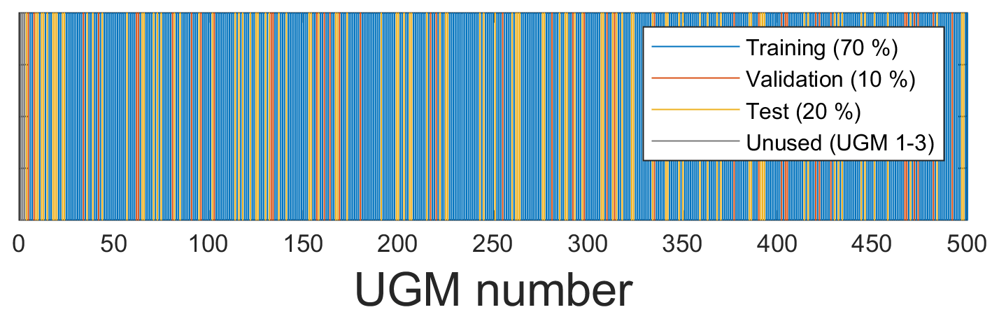
Figure 5 Randomized split of the UGMs into training, validation, and test data used in this contribution.

A 10-fold stratified CV is automatically performed in the AMLT to determine the best FE algorithm out of five complementary FE methods. In contrast to the data split, which is carried out by omitting complete UGMs and used for performing group-based CV with validation data, the 10-fold stratified CV randomly omits individual TCs. The RMSE value resulting from the 10-fold CV is called the random CV error. To obtain quality information on the trained model, the differences between the predicted and the observed target values are measured using RMSE. The test RMSE (T − RMSE) results from applying the trained model to the test data. There can be a significant difference between a group-based CV error and T − RMSE, as the omitted UGMs are selected randomly. For each of the five algorithm combinations (see Fig. 3), a Monte Carlo different train, validation, and test data sets, is performed. The mean value and standard deviation are calculated for the three different errors resulting from using training, validation, and test data, with n_comp=20 in the PLSR algorithm. The reason for choosing n_comp=20 is given below. The results are shown in Fig. 6. Although principal component analysis (PCA) achieves the lowest random CV error mean value (14.7 ppb), with negligible variations for different splits and therefore seems to be the best FE algorithm, applying 10 % validation data will lead to a group-based CV error mean value of 24.7 ppb. This means that 10-fold stratified CV does not efficiently detect overfitting for this application as it does not omit complete UGMs and, thus, does not need to interpolate to different gas concentrations. A new, unpublished version of the AMLT already allows the user to define validation scenarios (random or group based). Here, adaptive linear approximation (ALA) as the second-best method with a random CV error mean value of 15.3 ppb is chosen for further investigations as there is no significant difference in the error mean values between omitting single TCOs (15.3 ppb; random validation) and complete UGMs (16.5 and 16.6 ppb; group-based validation). Thus, it is sufficient to evaluate the random CV error with 80 % training (including 10 % validation data) and 20 % test data split by omitting complete UGMs in the training or test data, respectively. Applying this trained model (n_comp=20; 80 % data used for model training) to the 20 % test data (see Fig. 5) leads to a shown in Fig. 7.

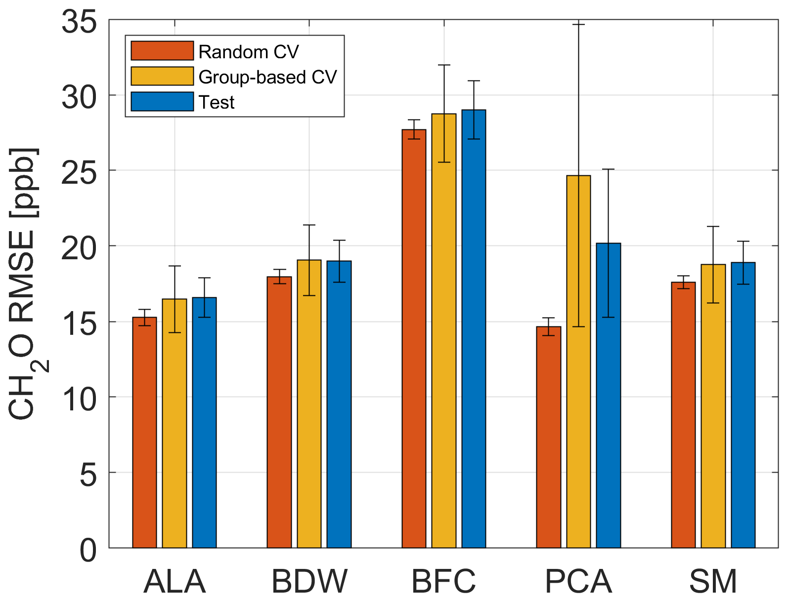
Figure 6 Random CV, group-based CV, and test RMSE of the five FE algorithms using Pearson as FS and PLSR with n_comp=20 for 100 trials with different randomized UGM splits and the formaldehyde concentration as target. ALA is the adaptive linear approximation, BDW is the best Daubechies wavelets, BFC is the best Fourier coefficients, PCA is the principal component analysis, and SM is the statistical moments.

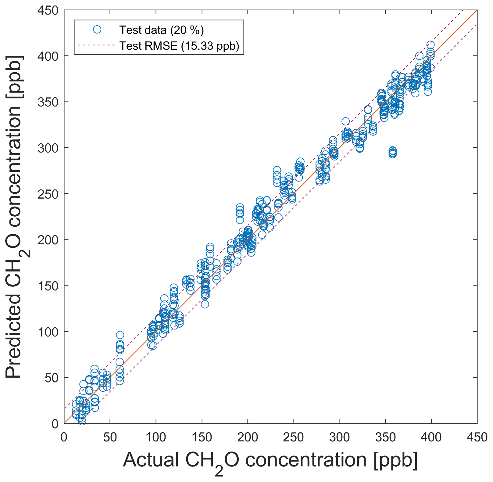
Figure 7 PLSR model for the quantification of formaldehyde for testing with test data from the data split shown in Fig. 5. Dashed lines indicate the RMSE of the test data (T − RMSE).

For VOC_sum as the target, the results are similar, and again, ALA is chosen as the best FE algorithm (random CV error mean value of 40.9 ppb) due to the overfitting of the trained model when using PCA (random CV error mean value of 31.9 ppb; group-based CV error mean value of 61.3 ppb). Applying the model trained with the data split in Fig. 5 to the 20 % test data results in a T − RMSE of 46.1 ppb. The corresponding results are shown in Figs. A3 and A4.

To determine the optimal number of PLSR components, a Monte Carlo simulation (10 trials with different train and test data) was carried out, and the T − RMSE mean values of 10 trials, in addition to the corresponding standard deviations, were calculated. In Fig. 8, the T − RMSE value is plotted over the number of PLSR components for ALA as FE, Pearson as FS, and PLSR. For a small number of PLSR components, T − RMSE mean values have large standard deviations, for example, the standard deviation for n_comp=1 is σ=5.5 ppb. If the number of PLSR components is greater than 10, then the standard deviations are in the range from 1.15 to 1.22 ppb; thus, the obtained models are highly reproducible. The lowest T − RMSE mean value is achieved for a high number of PLSR components (here 13.5 ppb is achieved with n_comp=100), but it is preferable to find a good tradeoff between the accuracy and computational cost, as a lower number of PLSR components reduces the computational effort. Therefore, the optimal number of PLSR components is determined using the elbow method (Thorndike, 1953) to ensure a stable model, with a T − RMSE of 15.3 ppb. The elbow point, i.e., the point after which no further significant change occurs, is determined by using the ALA algorithm. ALA automatically determines four segments as being the best segmentation of the T − RMSE curve (see Fig. 8). Thus, the optimal number of PLSR components is n_comp=20, as more components have no considerable influence on the T − RMSE, leading to higher computational cost and also increasing the risk of overfitting.

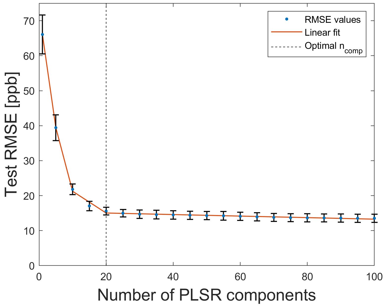
Figure 8 Elbow method applied to the T − RMSE curve for 10 trials. The optimal number of PLSR components is 20.

3.2 Influence of measurement uncertainty on ML results

In this contribution, two approaches for investigating the influence of the measurement uncertainty on machine learning results are considered, namely training a model with raw (see Sect. 3.2.1) and noisy (see Sect. 3.2.2) data, respectively. The trained models are used to predict data with varying noise levels between 0 and 98 dB in both use cases. Training a model with raw data means that the uncertainty associated with the raw data is propagated through the UA-AMLT, which saves on computational cost, as no retraining is necessary if the uncertainty changes. To validate the UA-AMLT, training with the noisy data of different SNRs is carried out and compared to the results of the uncertainty propagation approach. The number of PLSR components (n_comp=20) determined with the elbow method is considered for formaldehyde and VOC_sum as the target. For formaldehyde, the number of PLSR components leading to the minimum T − RMSE value, i.e., n_comp=100, is also considered and compared to the results for

3.2.1 Model trained with raw data

The motivation for using raw data for training and noisy data for model application is the typical degradation of sensors over time (Jiang et al., 2006). To avoid a loss in sensor performance, periodical recalibration is typically required, which is often expensive and difficult or impossible to perform, as collecting sensors and sending them to the lab leads to the downtime of the IAQ monitoring system.

The test plus uncertainty RMSE (T + U − RMSE) is introduced as measure for the quality of the model considering the uncertainty values. This T + U − RMSE value is the sum of the two RMSE values obtained by the test of the model (T − RMSE) and by propagating the measurement uncertainty through the toolbox (U − RMSE), respectively. It is calculated according to the following:

$$\begin{array}{}\text{(24)}& {\displaystyle }{\mathit{d}}_{\mathit{u}}={\mathit{y}}_{\mathbf{pred}}+{\mathit{U}}_{{\mathit{y}}_{\mathbf{pred}}}\text{(25)}& {\displaystyle }{\mathit{d}}_{\mathit{l}}={\mathit{y}}_{\mathbf{pred}}-{\mathit{U}}_{{\mathit{y}}_{\mathbf{pred}}}\text{(26)}& {\displaystyle }{\text{RMSE}}_{\mathrm{T}+\mathrm{U}}=\left\{\begin{array}{ll}\text{RMSE}\left({\mathit{d}}_{\mathit{u}},\mathit{y}\right)& {\mathit{y}}_{\mathbf{pred}}\ge \mathit{y}\\ \text{RMSE}\left({\mathit{d}}_{\mathit{l}},\mathit{y}\right)& \text{otherwise}\end{array}\right.,\end{array}$$

where y∈ℝ^m and y_pred∈ℝ^m denote the actual and the predicted target, respectively. ${\mathbf{U}}_{{\mathit{y}}_{\mathbf{pred}}}$ contains the uncertainty values associated with the predicted target. Furthermore, noisy data RMSE (ND-RMSE) is used, which indicates the quality of the model when applying it to another simulated data set (2000 cycles) with the added white Gaussian noise (noisy data) of different SNRs.

First, it is of interest if the selected FE algorithm still performs well when applying the model trained with raw data on noisy test data. ALA was chosen as the best FE algorithm when applying a model trained with raw data on raw test data, as shown in Sect. 3.1. Applying the model on noisy test data leads to the T + U − RMSE curves, as shown in Fig. 9. For SNR values greater than 65 dB, ALA achieves the smallest T + U − RMSE. In this range, the statistical moments (SM) also perform well, with the best Daubechies wavelets (BDW) achieving similar results for very high SNR≤85 dB. The T + U − RMSE difference between ALA (best algorithm) and SM is only 1.9 ppb for 98 dB. Between 50 and 65 dB, the smallest T + U − RMSE is achieved using statistical moments. If SNR≤50 dB, then PCA achieves the smallest T + U − RMSE. This means that PCA can compensate for noise in this range, but overfitting leads to higher error, as shown above for the raw data. This figure shows that the measurement uncertainty has a direct influence on the performance of the ML algorithm, and thus, different FE methods should be chosen for different SNR values.

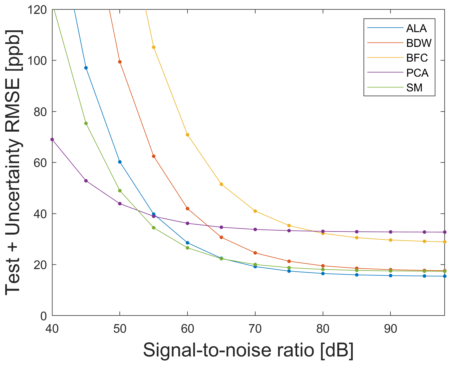
Figure 9 Test plus uncertainty RMSE (T + U − RMSE) curve for the five complementary FE algorithms, each in combination with the Pearson correlation for FS and PLSR.

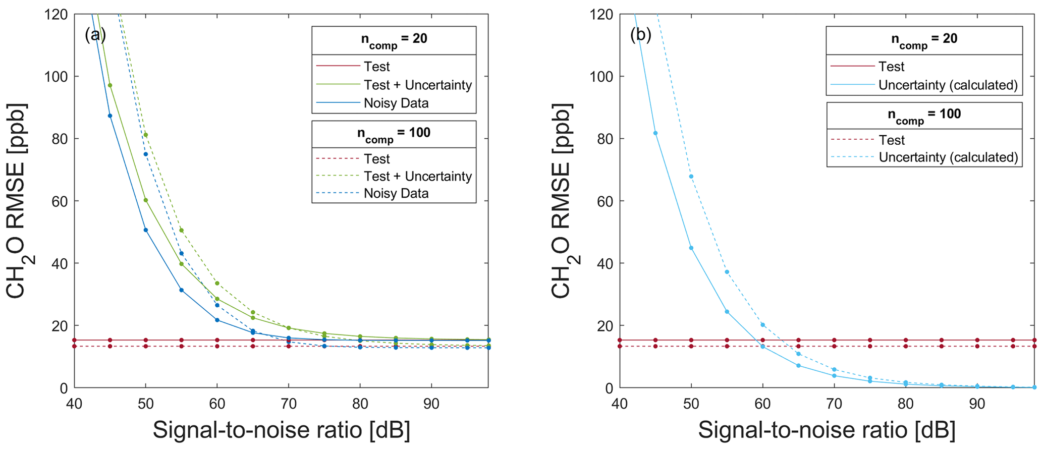
Figure 10 RMSE for testing a model trained with 80 % raw data for formaldehyde prediction on (a) 20 % test data without (red) and with associated uncertainty values (green), in addition to the application of the model on a noisy data set (blue) and (b) 20 % raw test data (red), and the calculated uncertainty RMSE (light blue) resulting from the difference in T + U − RMSE and T − RMSE for a different number of PLSR components.

Figure 10a shows T − RMSE, T + U − RMSE, and ND-RMSE values for a model trained on raw data for SNR≥40 dB (approx. maximum theoretical SNR for a 6 bit ADC, according to Eq. 21), using the data split shown in Fig. 5 with ALA as FE, the Pearson correlation for FS, and PLSR. The T − RMSE values in Fig. 10 are constant because the model was trained with one specific raw data split (see Fig. 5). For large SNR values, it can be assumed that the added white Gaussian noise is smaller than the SNR of the raw data and, therefore, has no significant influence, as is indeed observed. The T + U and ND errors show a similar increase with reduced SNR for both models with 20 and 100 PLSR components, with the ND error being slightly lower than the T + U error. This indicates that the model uncertainty estimated by propagating the error through the toolbox, i.e., the T + U error, overestimates the true model uncertainty slightly but still provides valuable insight into the sensitivity of the ML model to noisy data. To obtain an accurate model for predicting formaldehyde concentrations with n_comp=20, the SNR of the data set should not fall below 70 dB, as, for this SNR, the T + U − RMSE is approx. 19.2 ppb, which is an acceptable uncertainty for determining the formaldehyde concentration with a threshold limit value (TLV) of 81 ppb. An SNR of 45 dB for n_comp=20 and of 50 dB for n_comp=100 results in T + U − RMSE and ND-RMSE values of approx. 80 ppb, i.e., similar to the TLV, which means that the sensor system would no longer be useful for estimating the formaldehyde concentration. For SNR<80 dB, the model based on 20 PLSR components is more robust against noise than a model with 100 PLSR components, yielding lower RMSE values. In contrast, for SNR≥80 dB, a higher number of PLSR components performs slightly better, i.e., an improvement in the RMSE values can be achieved with more PLSR components if the noise level in the data is very low. In the case of an SNR value of 98 dB, the T − RMSE value is 15.33 and 13.34 ppb for n_comp=20 and n_comp=100, respectively.

Figure 10b shows the T − RMSE and the U − RMSE. U − RMSE is calculated as the difference between T + U − RMSE and T − RMSE (see Fig. 10a). This figure shows that the influence of the trained model (expressed by T − RMSE) on T + U − RMSE is constant, while the influence of the measurement uncertainty (expressed by U − RMSE) decreases steadily with increasing SNR. For n_comp=20 (n_comp=100), U − RMSE is smaller than T − RMSE when SNR is greater than 60 dB (65 dB).

The results for the additive white uniform noise and formaldehyde as target are nearly the same as for the additive white Gaussian noise (see Fig. A8a). Similar results for VOC_sum as the target are shown in Fig. A5a.

To demonstrate the effect of the noise on test data, PLSR models trained with raw data (n_comp=20) for the quantification of formaldehyde and VOC_sum are shown in Figs. A1 and A6 for the two different SNR values, respectively.

3.2.2 Model training with noisy data

The second use case occurs when using low-performance sensors or sensor systems that provide significant noisy data or where the electronics/ADCs add significant noise. For the investigation of the influence of measurement uncertainty on regression results, ALA as FE and Pearson correlation as FS are used together with PLSR. Formaldehyde as the target is discussed here, as VOC_sum leads to similar results, which are shown in Appendix A2. Only results for white Gaussian noise are shown here, as the results for white uniform noise are similar (see Appendix A3).

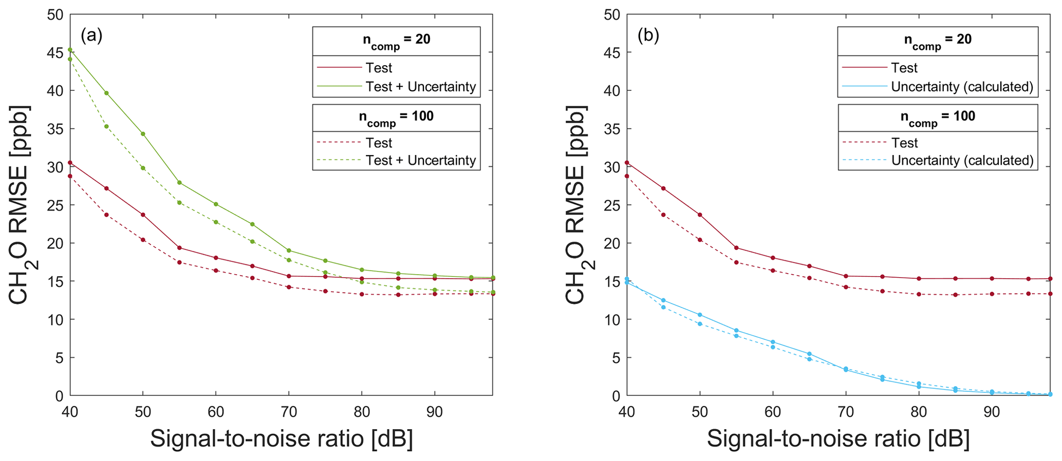
Figure 11 RMSE for testing a model trained with 80 % noisy data for formaldehyde prediction on (a) 20 % test data without (red) and with associated uncertainty values (green) and (b) 20 % raw test data (red) and the calculated uncertainty RMSE (light blue) resulting from the difference in T + U − RMSE and T − RMSE for a different number of PLSR components. Note the magnification compared to Fig. 10.

Figure 11a shows T − RMSE, T + U − RMSE, and ND-RMSE values for a model trained on noisy data for SNR≥40 dB, using the data split shown in Fig. 5. Compared to Fig. 10a, the T + U − RMSE is significantly smaller for the model trained with noisy data, i.e., the ML model can suppress noise if it is contained in the training data. For example, for SNR=50 dB and 20 PLSR components, the T + U − RMSE is 60.22 ppb when training with raw data, while it is only 34.3 ppb when training with noisy data. In general, a model can be made more noise resistant by adding additive white Gaussian noise to the training data. Comparing Figs. 10a and 11a, note that the regression results are similar for noisy and raw data for SNR≥80 dB, thus indicating again that the noise level of the raw data is approx. 80 dB. The same holds for T + U − RMSE when SNR≥80 dB. Of course, there is no need to train the model with noisy data with an added noise level lower than the noise of the original data. As already observed for the model trained with raw data, the RMSE values can be reduced by using more components, but here, this observation holds for all SNR levels, as the noise is contained in the training data, so there is no overfitting. This means that training a model with raw data once is sufficient, and no new model must be trained with noisy data. The associated measurement uncertainty values must only be used in the application of the model, which saves much computational cost. Figure 11b shows that, for T + U − RMSE values, the contribution resulting from the measurement uncertainty is always lower than the contribution from the test of the model. This means that the noise is already trained in the model, and improving the used sensor would significantly improve the ML results.

For white uniform noise, similar results are shown in Fig. A8b.

In case of VOC_sum as the target, the results are similar, despite the fact that the RMSE values are higher than for formaldehyde, as shown in Fig. A5b. No significant difference between the RMSE values when training with raw and noisy data, respectively, is observed for SNR values higher than 70 dB.

To demonstrate the effect of noise on test data, PLSR models trained with noisy data (n_comp=20) for the quantification of formaldehyde and VOC_sum are shown in Figs. A2 and A7, for two different SNR values, respectively.

4 Conclusion and outlook

In this contribution, the uncertainty-aware AMLT for classification tasks presented in Dorst et al. (2022) was first extended for solving regression problems. In accordance with the GUM, an analytical method for uncertainty propagation of PLSR was implemented. The code for this UA-AMLT for classification and regression tasks was published on GitHub (https://github.com/ZeMA-gGmbH/LMT-UA-ML-Toolbox, last access: 18 January 2023). For different SNR levels, the UA-AMLT automatically selects the best ML algorithm based on the overall test plus the uncertainty RMSE.

The influence of measurement uncertainty on machine learning results is investigated in depth with two use cases, namely model training with raw and noisy data generated by adding white Gaussian noise. For both use cases, the analysis shows where the measurement system must be improved to achieve better ML results. In general, there are two distinct possibilities, i.e., improving either the ML model or the used sensor. In case of an RMSE resulting from measurement uncertainty tending towards zero, an improvement of the ML model is suggested. In the range where U − RMSE is already very small (see Fig. 10b), a better ML model should be obtained as optimizing the sensor, including the data acquisition electronics, will only lead to even lower U − RMSE values close to zero, which does not significantly impact the overall T + U − RMSE. In contrast to that, in ranges where U − RMSE is higher, minimizing this RMSE by optimizing the physical sensor system should be the objective. To reduce the T − RMSE resulting from the ML model, using a better model would be necessary, as this can significantly influence the ML results. A better model can be achieved, for example, by using a higher number of PLSR components, as shown in this contribution, or by using deep learning, which can also improve the T − RMSE (Robin et al., 2021).

Finally, it is shown that increased robustness of the machine learning model can be achieved by adding white Gaussian noise to the raw training data.

In future work, the influence of different types of colored noise on ML results can be investigated, as this contribution has addressed only different additive white noise models. Therefore, the correlation must be considered within the uncertainty propagation, and this is only possible for the feature extractors. Furthermore, the difference between noise produced by the data acquisition electronics, especially the logarithmic amplifier as simulated in this contribution, and noise produced by the sensor could be investigated. To simulate sensor noise or electronic noise before the logarithmic amplifier noise, the noise must already be added to the inverse logarithmic of the logarithmic resistance raw data.

Appendix A: Additional figures

A1 Formaldehyde as target

Figure A1 PLSR model (trained with raw data; n_comp=20) applied to test data (see Fig. 5) for the quantification of formaldehyde and the propagated uncertainty. (a) SNR=55 dB. (b) SNR=40 dB. Dashed red and green lines indicate the test RMSE (T − RMSE) and the test plus uncertainty RMSE (T + U − RMSE) based on test data, respectively. For better visibility, error bars are only shown for every 10th prediction.

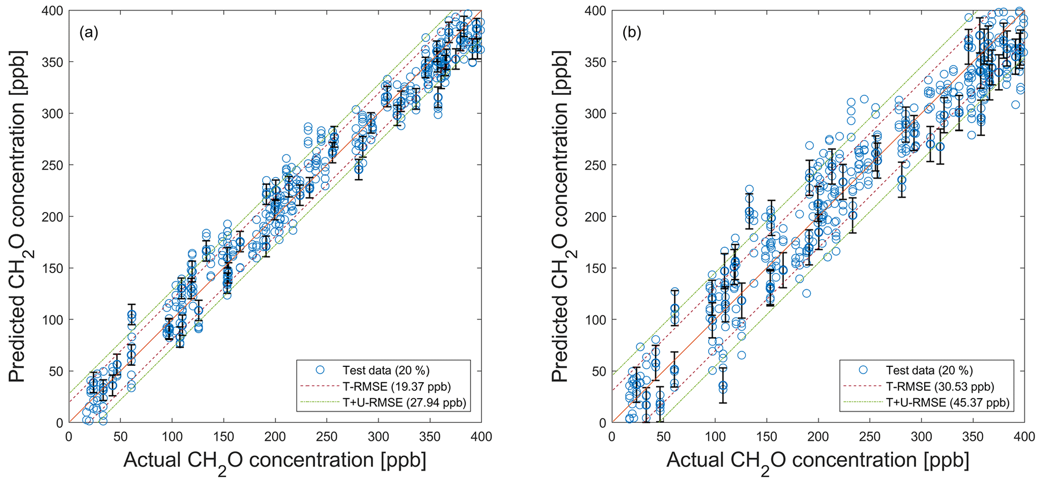
Figure A2 PLSR model (trained with noisy data; n_comp=20) applied to noisy test data (see Fig. 5) for the quantification of formaldehyde using their associated standard uncertainty. (a) SNR=55 dB. (b) SNR=40 dB. Dashed red and green lines indicate the test RMSE (T − RMSE) and the test plus uncertainty RMSE (T + U − RMSE) based on test data, respectively. For better visibility, error bars are only shown for every 10th prediction.

A2 VOC_sum as target

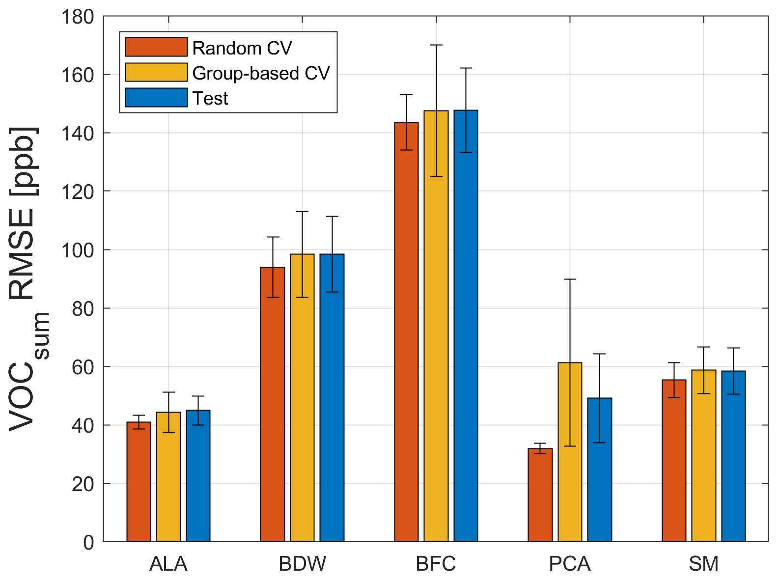
Figure A3 Random CV, group-based CV, and test RMSE of the five FE algorithms, using Pearson as FS and PLSR with n_comp=20 for 100 trials with different data splits and the VOC_sum concentration as target. ALA is the adaptive linear approximation, BDW is the best Daubechies wavelets, BFC is the best Fourier coefficients, PCA is the principal component analysis, and SM is the statistical moments.

Figure A4 PLSR model for the quantification of VOC_sum for testing with test data from the data split shown in Fig. 5. Dashed lines indicate the RMSE of test data (T − RMSE).

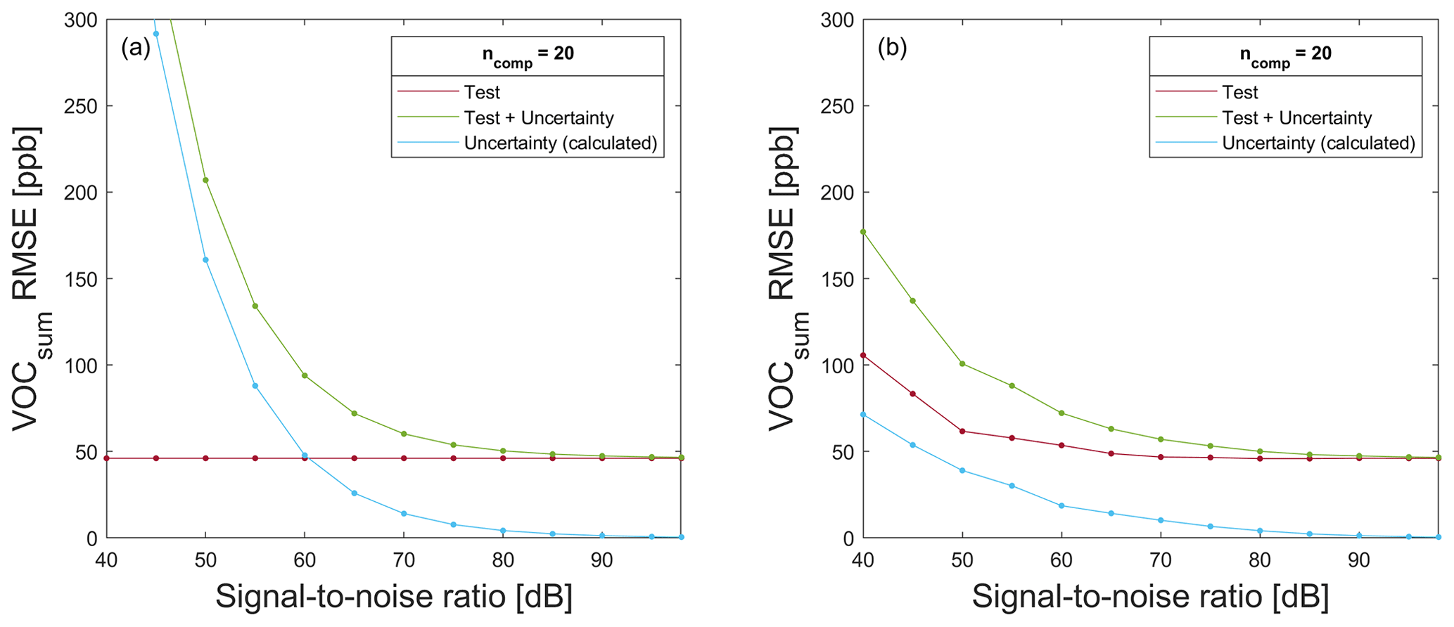
Figure A5 RMSE for testing a model trained with 80 % (a) raw data and (b) noisy data for VOC_sum prediction on 20 % test data without (red) and with associated uncertainty values (green), in addition to the calculated uncertainty RMSE (blue) resulting from the difference in T + U − RMSE and T − RMSE.

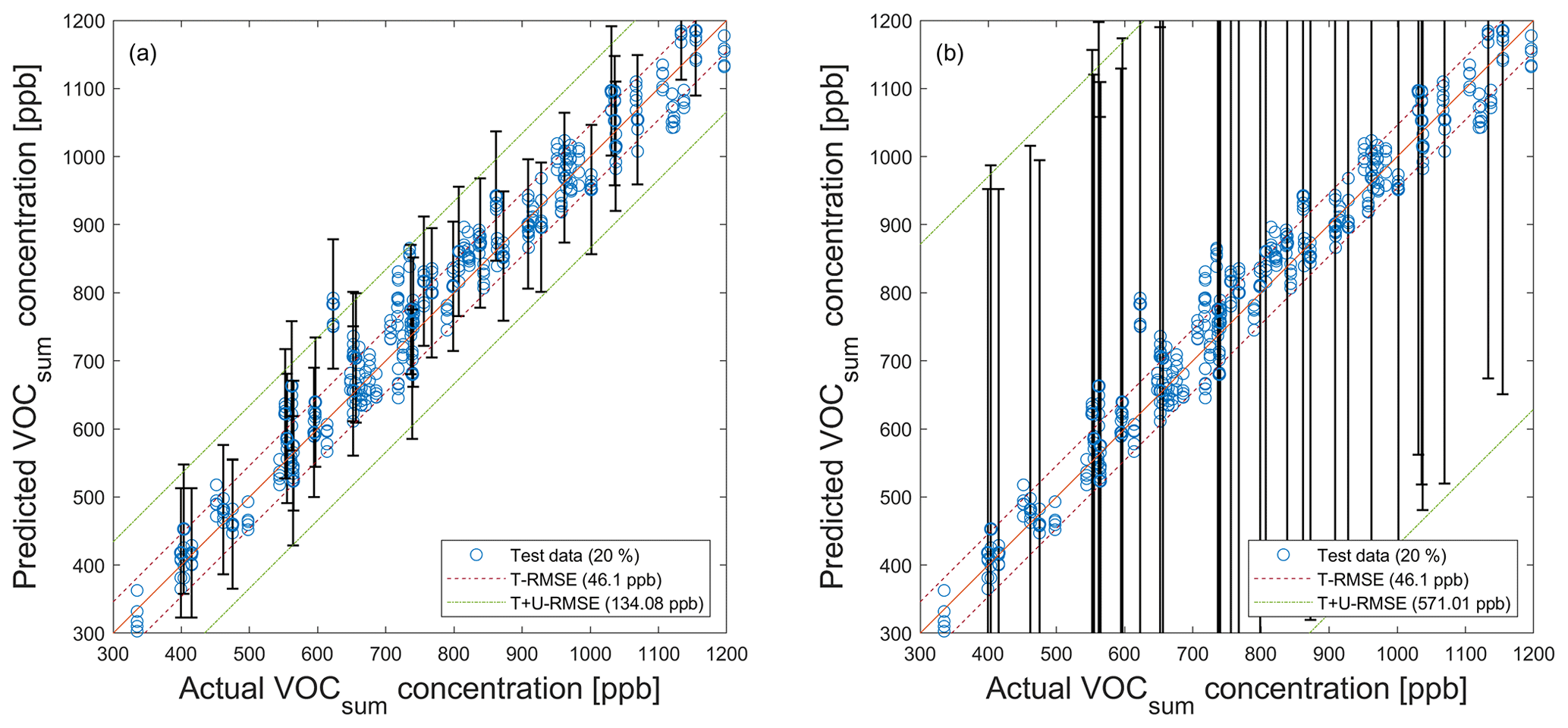
Figure A6 PLSR model (trained with raw data; n_comp=20) applied to test data (see Fig. 5) for the quantification of VOC_sum and propagated uncertainty. (a) SNR=55 dB. (b) SNR=40 dB. Dashed red and green lines indicate the test RMSE (T − RMSE) and the test plus uncertainty RMSE (T + U − RMSE) based on test data, respectively. For better visibility, error bars are only shown for every 10th prediction.

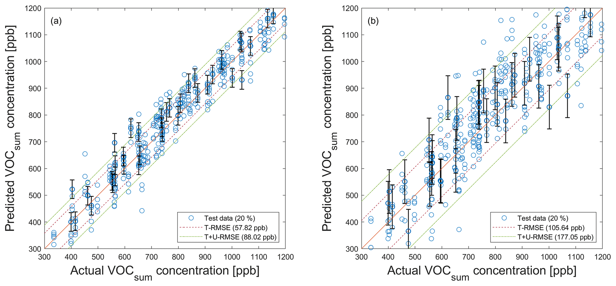
Figure A7 PLSR model (trained with noisy data; n_comp=20) applied to noisy test data (see Fig. 5) for the quantification of VOC_sum using their associated standard uncertainty. (a) SNR=55 dB. (b) SNR=40 dB. Dashed red and green lines indicate the test RMSE (T − RMSE) and the test plus uncertainty RMSE (T + U − RMSE) based on test data, respectively. For better visibility, error bars are only shown for every 10th prediction.

A3 Additive white uniform noise and formaldehyde as target

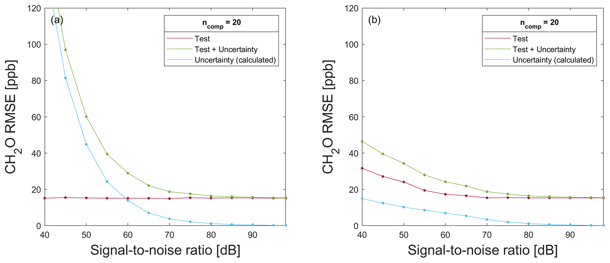
Figure A8 RMSE for testing of a model trained with 80 % (a) raw data and (b) noisy data (added white uniform noise to raw data) for a formaldehyde prediction on 20 % test data without (red) and with associated uncertainty values (green), in addition to the calculated uncertainty RMSE (blue) resulting from the difference in T + U − RMSE and T − RMSE.