the Creative Commons Attribution 4.0 License.
the Creative Commons Attribution 4.0 License.
 | 30 Apr 2024
Simple in-system control of microphone sensitivities in an array
Artem Ivanov
A method to perform measurements of microphone responses directly in the array of a sensor system is described. It can be applied in reverberant environments and does not require high instrumentation effort. Due to the use of internal hardware of the sensor system, the whole signal chain of microphone–preamplifier–analogue-to-digital converter is characterized. The method was successfully tested for calibration of two types of planar arrays constructed with micro-electromechanical system (MEMS) microphones. Presented experimental results illustrate achieved performance, and possible application scenarios are discussed.
- Article
(4353 KB) - Full-text XML
- BibTeX
- EndNote


Microphone arrays are widely used in acoustic measurements. An example can be found in acoustic cameras, where a suitable combination of single-sensor signals allows users to localize sound sources with the help of beam forming or to reconstruct the sound field by use of acoustic near-field holography. Further examples are discussed, for example, in Brandstein and Ward (2001). The processing algorithms rely on exact matching between the microphones or at least on the knowledge of their amplitude and phase responses to compensate for the differences; therefore, extensive research was devoted to methods of calibrating microphone arrays (Tashev, 2004; Zuckerwar et al., 2006; Szőke et al., 2022).
Microphone sensitivity is usually defined in the laboratory either by a comparison with a reference microphone, by substitution or using the reciprocity approach; in the field the use of a pistonphone is typical (Brüel & Kjaer, 2019). The calibration task becomes especially challenging when the single microphones cannot be removed from the array after the assembly, e.g. when the array is built of miniature micro-electromechanical system (MEMS) devices soldered onto printed circuit boards (Perrodin et al., 2012). In multi-channel condenser microphone systems, verification of single-channel functions can be performed using, for example, the actuator method, the insert voltage or the charge injection calibration methods (Brüel & Kjaer, 2019). These methods are, however, not directly applicable to the MEMS microphones.
The approach proposed here allows for a direct in-system verification of amplitude responses of the MEMS microphones. So control of the actual condition of the microphone array is possible. The method can be used with a simple hardware that is capable of acquiring and processing signals at low sample rates only and was successfully tested with planar arrays in reverberant sites. Although specific target applications were initially considered, the method can be useful for other multi-microphone systems.
The presented method to measure microphone sensitivities in an array was developed and tested within a project targeting a system for visualization of surface vibration patterns based on the acoustic vibrational mode tracking (AVMT) technique (Ivanov and Kulinna, 2023). For a better understanding of the hardware parameters and of the physical background, a short outline of the system hardware and measurement principle will be given.
Two tested sensor systems are shown in Fig. 1. The systems are equipped with a high number of miniature omnidirectional microphones (128 and 192 devices) arranged in close pairs to form discrete pressure gradient probes, below referred to as “measurement channels”. The used MEMS microphones have a low height of 1 mm and are mounted on printed circuit boards at 3 mm distance from each other, as can be seen in the inset in Fig. 1a. During a measurement, the circuit boards are placed in the sound wave with their surface parallel to the wave propagation direction, so the disturbance to the sound field is kept at a minimum. The difference of the microphone signals in the pair can be used to estimate the sound pressure gradient in the direction of their displacement. From this value, the particle velocity in the sound wave can be calculated. If the sound wave is created by a vibrating object surface situated close to the measurement array, the calculated particle velocities are assumed to be defined by the motion of the object surface. Measurements performed simultaneously by different channels would deliver an estimation of the current vibrational state of the object. This would allow contactless measurement of vibrational modes excited by single non-reproducible events that cannot be acquired by scanning laser Doppler vibrometers. In comparison to the related method of acoustic near-field holography, it is expected that the lower calculation complexity and the robust algorithm of the proposed approach would allow for live visualization of non-stationary vibrations.
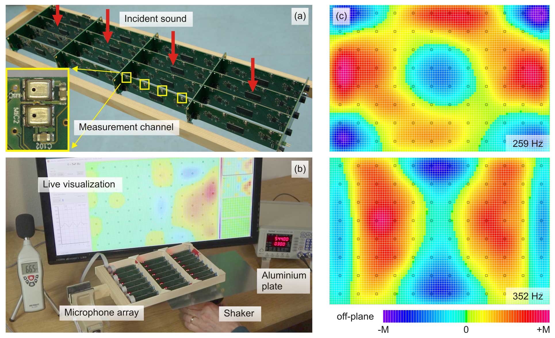
Figure 1(a) Sensor system (System A) with 64 channels. Inset: a close-up view of a measurement channel; spacing between the microphone input ports is 3 mm. (b) The experimental set-up for measurement of plate vibration modes. Here a system with 96 channels (System B) is used with an aluminium plate (250 mm×167 mm, 0.5 mm thick) that is driven in its centre by a shaker. (c) Colour-coded representation of the normal plate modes acquired with a sine wave excitation at 259 and 352 Hz. The grid of black squares indicates the positions of measurement channels; values between the grid points are interpolated. Colour scale maximum M for the off-plane displacement amplitude amounts to M=400 a.u. (at 259 Hz) and M=500 a.u. (at 352 Hz).
Currently the sensor systems are under evaluation, so the applicability and limitations of this approach are still to be defined. Figure 1c gives preliminary results illustrating some of the acquired normal plate modes measured in the set-up shown in Fig. 1b; a more detailed analysis and the validation of the results will be presented elsewhere (Ivanov, 2024).
The proposed measurement principle relies on calculating differences between the microphone signals in the pairs and so implies matched sensitivity of the involved microphones. As experiments showed, the sensitivity spread of low-cost MEMS microphones in the array was too high to allow for their direct use without calibration. The initially considered calibration option was to measure the microphone responses in a standing-wave tube. Alternatively, measurements in an anechoic chamber were discussed. Although the calibration results in the standing-wave tube were sufficiently good for the application, the practical effort was found to be high: because of the size limitations of the available equipment, the microphone array had to be first taken apart and then board-wise calibrated and, at last, assembled back to the original grid geometry.
To reduce the calibration effort, the method described in Sect. 3 was proposed. It allows users to determine microphone sensitivities directly in the array without the need of an anechoic chamber or other special equipment. The method was successfully tested with both hardware variants (“System A” and “System B” as they are referred to below), which differed not only in their geometry and digital signal processing capabilities but also in the complexity of their analogue front ends.
The microphone array of System A contains 128 consumer-grade MEMS microphones (SPW0442, Knowles) placed in a rectangular grid configured into a 16 by 4 channel matrix of 30 mm spacing (Fig. 1a). This system is designed for acquisition of both stationary and transient processes and is equipped with a large data storage capacity. It consists of identical sensor boards, several connector boards to set up the sensor array, and a master board which controls the measurement process and transfers the results to a PC. Each sensor board contains four measurement channels (made up of two microphones each), two four-channel 24-bit audio analogue-to-digital converter (ADC) ICs (CS53L30, Cirrus Logic) and a microcontroller (ARM Cortex M4 STM32F446, STMicroelectronics) to process the signals. The AD conversion of the audio signals is performed at 48 ksps (kilo-samples per second); measurement sequences of up to 43 s duration can be stored locally on the board.
The second hardware variant – System B (Fig. 1b) – targets low complexity and cost. Due to the simplified electronics, it is only capable of visualizing quasi-stationary vibrations. In this system, each sensor board also carries eight MEMS microphones; their signals undergo amplification and filtering by a simple operational amplifier circuit (MCP6004, Microchip) and are digitized by the internal 12-bit AD converter of a 16-bit microcontroller (dsPIC33E, Microchip). The microphone signals are sampled sequentially in a loop with the effective throughput of 40 ksps. In the presented experiments, the array of System B contained 192 microphones in total and was configured in a matrix of 12 by 8 channels with 20 mm spacing.
The proposed method targets the case when the microphones cannot be removed from the array for calibration, so the acquisition of their responses is performed directly within the sensor system itself. Due to this approach, the influence of the whole acquisition chain of microphone–preamplifier–ADC is taken into account.
To cope with the practical situation of reverberant environments, sound sources generating waves with a distinguished first wavefront were used. The underlying idea is to concentrate the signal processing onto this first wavefront and so to effectively suppress reflected and scattered waves that reach the microphones later. A short estimation helps to illustrate the timing requirements: in 1 ms a sound wave travels about 34 cm in the air, so using sound waves with the first wavefront duration in the order of 0.1 ms limits the zone, where the disturbing reflections can originate from, to approximately 3 cm from the microphone. Knowing the geometry of the array and the anticipated sound pressure distribution on its elements (e.g. from a simulation), measurement of the microphone responses can be carried out. The results presented below were obtained using the simplified approach, assuming a uniform pressure distribution over all microphones in the array and modelling the sound wave as it would be created by a distant point source.
A suitable source of such an explosion-like excitation can be, for example, a popping balloon or hands clapping. Characteristics of laser-induced plasma discharges described in Szőke et al. (2022) would probably allow users to use this phenomenon as a reliable excitation source. The most practical source in our tests turned out to be a loudspeaker driven with a voltage pulse. An example of the related microphone signal is given in Fig. 2. It was obtained using a loudspeaker (60 W, 4 Ω, 5 in. woofer from JBL GTC5210) positioned 3 m away from the array and driven by a rectangular voltage pulse of 15.5 V amplitude. It can be seen from Fig. 2 that the microphone signal exhibits a peak with duration of approximately 8 samples (about 180 µs), corresponding to the first wavefront.
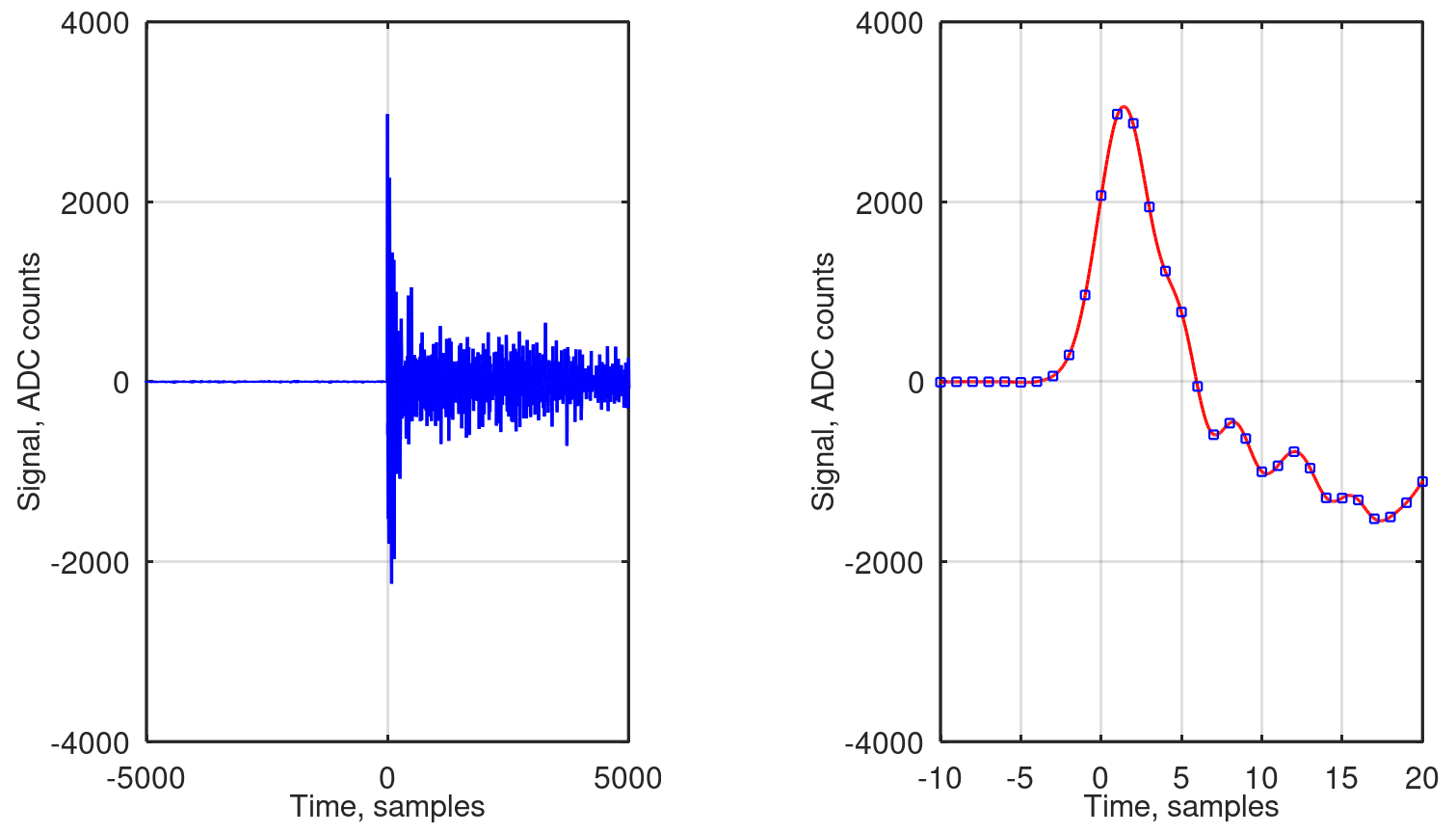
Figure 2Microphone signal recorded at 48 ksps and its interpolation shown with different time scales. A loudspeaker driven by a rectangular voltage pulse was used as the sound source.
As described in the previous section, the target hardware performs signal sampling at frequencies typical for audio recording (40 and 48 ksps; see Sect. 2); it is hence too slow to acquire the shape of the first signal peak with necessary details and accuracy. Achieving a sufficiently high sampling frequency is, however, not possible with targeted low-cost hardware solutions. To overcome this limitation, the recorded signals are interpolated in the time domain before processing as illustrated in the right plot of Fig. 2. It is important, however, that the microphone signals are sufficiently low-pass filtered and do not exhibit aliasing effects after sampling. At last, the maximum and arrival time of the first peak are defined from the interpolated signal. After performing measurements on several sound pulses, the average values are calculated and used to determine the relative sensitivities of the array of microphones.
The microphones have a flat frequency response from 50 Hz (−3 dB) to 10 kHz (+3 dB) and a +20 dB peak at 20 kHz. The corner frequency of the anti-aliasing filter was set to 19 kHz for System A and to 9 kHz for System B. Together with the high-pass filtering needed to remove the low-frequency noise, a band-pass filter for the microphone signals was formed. The high-pass corner frequency of 900 Hz was used in our measurements.
This procedure of defining microphone sensitivities cannot be called calibration in the strict sense. First of all, it does not include the frequency dependency. Additionally, the microphone properties are measured in a mounted state with possible interference of the printed circuit boards, the wave incidence angles are not accounted for, etc.
As long as the microphone signals are sampled without violation of the Nyquist–Shannon theorem and so no aliasing takes place, the signal can be reconstructed in all details using the so-called ideal interpolation. It can be performed either by zero padding in the frequency domain or by a convolution with the (actually infinitely long) Sinc-kernel in the time domain. This method is, however, of limited value if it is to be done in real time during the acquisition of the signals. Interpolation with several popular kernels (Burger and Burge, 2013) that can be implemented on systems with very limited hardware resources (e.g. System B) were tested. The goal was to provide a good substitution for the ideal interpolation. Some of the test results are shown in Fig. 3 in comparison; here once more, a signal from a loudspeaker sound pulse recorded at 48 ksps is presented. The most convincing interpolation results were obtained using convolution with the Lanczos kernel. In the subsequent steps, the Lanczos kernel of seventh order was used.
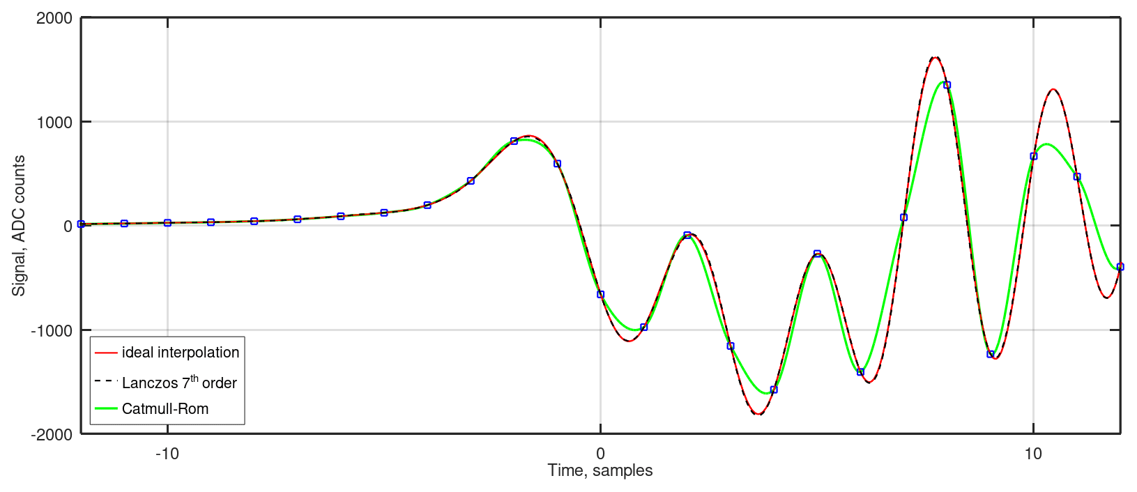
Figure 3Three interpolation methods in comparison. A sound pulse produced by a loudspeaker is shown, sampled at 48 ksps.
The below-presented measurements of microphone responses were carried out with the loudspeaker (specified in Sect. 3) as the excitation source. It was placed at a distance of 2 m (data in Figs. 4, 5 and 7) or 3 m (data in Fig. 6) from the sensor system and driven by connecting it to a 4700 µF capacitor charged to 15.5 V. The relative positions of the loudspeaker and the microphone array were adjusted to achieve an almost normal sound wave incidence upon the array. All measurements were performed in ordinary (reverberant) locations not actually intended for acoustic experiments; the highest possible repetition rate of the sound pulses to suppress effects due to the echoing was found to be 2 Hz. For a better control of the experiment, the sound pulses were typically generated with a delay time of 5 s.
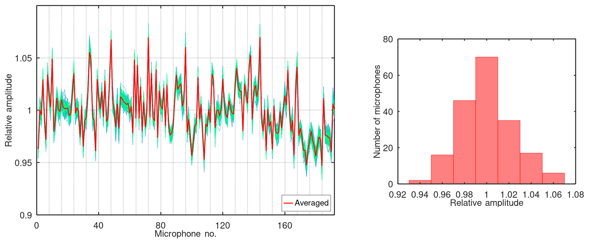
Figure 4Relative amplitude responses of 192 microphones in the array. Results of 100 measurements are presented with line colours ranging from blue to green. The average over all measurements is shown in red in the plot and in the histogram.

Figure 5Variation of relative amplitude responses of selected microphones in subsequent measurements. Three different averaging approaches are compared: cumulative average (red) and Butterworth infinite impulse response (IIR) filters of first (blue) and second (green) orders with characteristic times of 50 and 25 measurements, respectively.

Figure 6(a) First wavefront arrival time in comparison with the theoretical curve. (b) Effect of a dirt particle partially obstructing the microphone port on the measured wave arrival time, indicated with a green circle.

Figure 7Arrival time of a sound pulse for two array lines (line 1 is in the foreground of the photograph). Results of 100 measurements are presented with line colours ranging from blue to green. The averages over all 100 shots are given by the red and black lines.
The microcontrollers of the sensor system executed a dedicated software branch that allowed them to automatically detect the first wavefront of the sound pulse, to pre-process the signal (perform digital filtering and interpolation) and to define the amplitude of the first signal peak as well as its arrival time for all microphones. As a result, after every sound pulse a data set was generated and transferred to a control PC that contained the amplitude and time information for all array microphones. These single measurements will be also denoted as “shots” in the discussion below. In each geometrical configuration, the shots were repeated at least 100 times to get a sufficient data basis for evaluation.
Figure 4 shows a distribution of the microphone amplitude responses in the sensor array of System B with 192 microphones. The relative amplitude responses are calculated with respect to the average amplitude over all array microphones measured in one shot (i.e. after recording of one sound pulse). Here a data set with 100 shots is presented. Every single measurement is plotted with a blue-to-green line connecting the relative responses of all microphones in the rising order of their identification indexes. The colour of the connecting line is unique for a shot. The blue–green stripe formed as a result of plotting all 100 measurements in a stack indicates the uncertainty observed in this experiment. In spite of conducting measurements in a reverberant room and despite the strong undersampling of the microphone signals and the necessity of subsequent interpolation, the reproducibility of data is quite high as indicated by a low width of the blue–green stripe, which is about 2 %. Most of this spread is presumably due to the interpolation of the signal, as the noise of the system as revealed by measurements performed on lower-frequency signals lies substantially below this value.
The red line in Fig. 4 represents the relative amplitude response of the microphones averaged over 100 shots. These values form the basis for calculation of sensitivity correction coefficients for single microphones as needed in the target application described in Sect. 2. The effect of using these coefficients will be illustrated below in Fig. 8.
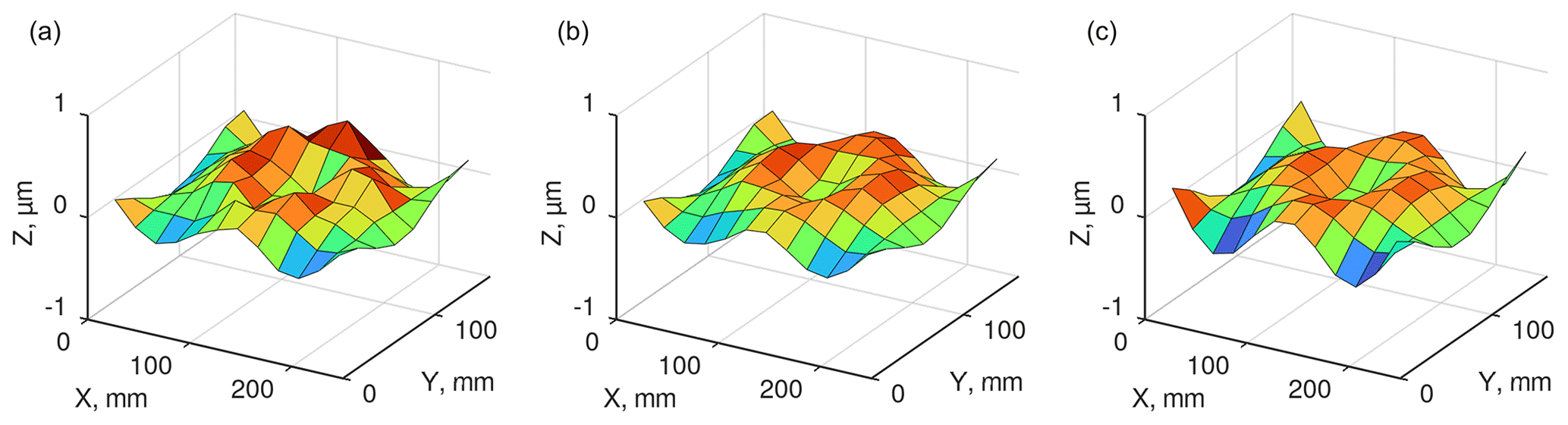
Figure 8Vibrational mode of an aluminium plate () driven by a sine wave at 547 Hz as acquired by System B without (a) and with (b) correction of microphone sensitivities. The same vibration measured with a scanning laser vibrometer on identical grid (c).
According to the data sheet of the utilized MEMS microphones (Knowles, 2018), their sensitivity amounts to −42 ± 1 dBV Pa−1 (reference value of 1 V), which is approximately equivalent to a spread of ±12 % on the amplitude scale. It can be seen from Fig. 4 that measured sensitivities lie well within the anticipated range.
Especially when low-cost microphones are used in an application, their temperature stability or ageing effects must be carefully considered. The proposed method allows for continuous control of the amplitude responses of microphones already installed in an array and could be used, for example, for a drift compensation. To implement this correction, the software controlling the sensor system should be transferred into a calibration mode to record a dedicated sound pulse or a pulse sequence. As drift effects are usually slow, only a small percentage of working time of the system needs to be devoted to the calibration activities. A possible scenario could be to process one calibration event with 1 s duration once a minute and to feed its results into a digital filter tracking the system state.
To illustrate the variation of measurement results, the relative amplitude responses acquired in 100 subsequent shots are given in Fig. 5. From the total of 192 microphones of the system shown in Fig. 4, three were selected to represent the average, the minimum and the maximum sensitivity ranges. The coloured lines illustrate different possibilities to obtain a stable value from the varying results of single measurements. The red line stands for a cumulative average; it allows users to visually estimate how many measurements must be performed so that their mean value becomes stable. As can be seen from Fig. 5, the cumulative average does not vary much after completion of 20 measurements. This indicates that it would be sufficient to acquire data of just 20 shots to come to stable mean values. The value of the cumulative average by the end of 100 shots coincides with the simple averaging over these measurements as it was used for the data in Fig. 4.
In the right plot, the action of two exemplary digital filters upon the original results is presented; such filtering could be more suitable for tracking slow changes than the simple averaging. As the input data, the sensitivity of only one microphone (Mic. 2) is shown here. There exist numerous variants of digital finite impulse response (FIR) and IIR filters that could be used for the tracking, with, for example, the moving average as one of the simplest. The right plot shows the filtering results achieved with Butterworth filters of the first (blue) and second (green) orders with time constants of 50 and 25 measurements, respectively. They reach steady states after approximately 60 to 80 shots and deliver a smoothed representation of the incoming measurement results. The initialization of the filters was performed here according to Likhterov and Kopeika (2003). The choice of the filter characteristics must be done according to the requested control period and anticipated change rates in a specific application.
The arrival time of the first wavefront is plotted in Fig. 6 for exemplary measurements. The data in the left plot were acquired using System A in the form as it is depicted in Fig. 1a: the sensor boards were arranged into four parallel lines at a distance of 30 mm from each other. Only values corresponding to the microphones of the front array row are shown for clarity. Note the sub-sample resolution on the time axis which is possible due to the interpolation of the signals. The interpolation was performed by a factor of 16, theoretically leading to a 16 times higher resolution. The green curve shows the theoretically anticipated arrival time based on the point source model for the given geometry (the speed of sound was taken to be 344 m s−1). A good agreement with the simple theoretical model can be observed.
The right plot in Fig. 6 was acquired with System A configured into lines consisting of three sensor boards. Here both the front and the rear microphones of one line are presented. It can be clearly seen that the wave arrival time measured by one of the microphones (indicated by a green circle) stands out from the anticipated pattern. The inspection of the sensor boars performed after the measurement revealed a dirt particle which partially obstructed the input port of the concerned microphone. Although the time shift generated by the presence of the disturbing particle is well below one sampling period, the method is sufficiently sensitive to detect it. It is hence possible to also use it for the condition monitoring of the array: should the pattern of microphone reactions differ from the one measured with a definitively intact sensor system, an indication of possible malfunction can be triggered and the location of the probable point of failure defined.
The data given in Fig. 7 were obtained using System B in the configuration with eight lines of sensor boards containing three boards each (see the photograph in Fig. 7; the front array line is “line 1”). It is the same data set that was used for determining microphone sensitivities in Fig. 4. In a similar manner, the blue-to-green lines denote single measurements, and plotting data from all 100 shots on top of each other creates a blue–green stripe indicating the spread in results. The plotted data clearly deviate from the theoretical parabolic curves anticipated from the point source model. It is especially pronounced close to the centre of the array (array line 4) and for the rear microphones which are located 5 mm away from the board boundary.
This effect is most probably caused by the interference of the sound wave with the supporting structure and indicates that the mechanical construction of the microphone array can significantly influence the measured wave arrival time. It can be seen by comparing the photograph and the plots in Fig. 7 that the strongest deviation from the theoretical parabolic curve occurs close to the positions of the supporting bars in the array structure (horizontal grid lines in the plots).
Nonetheless, the wave arrival time remains reproducible from one shot to another as indicated by the relatively small width of the blue–green stripes created by the overlay of single plots. It confirms the possibility to use the method for condition monitoring of the array.
The vibration patterns presented in Fig. 8 were acquired with System B to prove the validity of the described approach for determining microphone sensitivity correction coefficients in the target application. The experimental set-up is of Fig. 1b: plate modes induced in an aluminium plate by a shaker were acquired by the microphone array situated above the plate; the array and the plate had effectively the same size. Figure 8b depicts the plate vibrational mode that was acquired using the calculated sensitivity correction coefficients; in Fig. 8a, the result of recording the same plate vibration with uncorrected microphone responses is shown. The true shape of this vibrational mode can be seen in Fig. 8c, it was acquired using laser Doppler vibrometry as a reference technique. Comparison of the three plots clearly shows that correction of microphone amplitude responses helps to achieve a good reproduction of the true vibration pattern.
The presented approach allows users to perform measurements of microphone responses directly in the array using the internal hardware of the sensor system. In this way, the whole signal chain starting from the microphone, including the filters and the preamplifier, and ending with the analogue-to-digital converter is characterized. The measurements do not need special equipment like an anechoic chamber and can be carried out in ordinary reverberant locations. The necessary excitation source producing sound waves with a short and well-formed first wavefront can be implemented using a loudspeaker driven by a capacitor discharge.
As experiments show, an estimation of the microphone sensitivity in the array can be performed with a sufficient precision to apply algorithms relying on the pair-wise subtraction of measured sound pressure values. If at least one of the array microphones is previously calibrated, it can be used as the reference for determining the absolute sensitivity of other microphones in the array.
Except for correction of microphone sensitivities, several possible application scenarios for the proposed method were identified. For example, it can be used for the compensation of drifts in the system caused by a temperature change or by the ageing of the components. Another possibility is to periodically monitor the system state to avoid incorrect measurements. Additionally, the sub-sample resolution of acquired time-of-arrival signals can be used for calibration of the array geometry.
The method can be realized with a low hardware effort: it was implemented in the full above-described scope on a 16-bit microcontroller with 32 kB flash memory and 4 kB RAM for processing of eight microphones at 40 ksps.
All relevant data presented in the article are stored according to institutional requirements and as such are not available online. However, all data used in this paper can be made available upon request to the author.
The author has declared that there are no competing interests.
Publisher's note: Copernicus Publications remains neutral with regard to jurisdictional claims made in the text, published maps, institutional affiliations, or any other geographical representation in this paper. While Copernicus Publications makes every effort to include appropriate place names, the final responsibility lies with the authors.
This article is part of the special issue “Sensors and Measurement Science International SMSI 2023”. It is a result of the 2023 Sensor and Measurement Science International (SMSI) Conference, Nuremberg, Germany, 8–11 May 2023.
The author would like to acknowledge Landshut University of Applied Sciences for financial and technical support and the companies Polytec GmbH and OptoMET GmbH for performing laser vibrometer measurements in their facilities.
The project and this open-access publication was funded by Landshut University of Applied Sciences.
This paper was edited by Gabriele Schrag and reviewed by three anonymous referees.
Brandstein, M. and Ward, D. (Eds.): Microphone arrays: Signal processing techniques and applications, Springer-Verlag Berlin Heidelberg, Germany, 398 pp., https://doi.org/10.1007/978-3-662-04619-7, ISBN 978-3-540-41953-2, 2001.
Brüel & Kjaer: Technical documentation, Microphone handbook, Vol. 1: Theory, BE 1447-12, https://www.bksv.com/doc/be1447.pdf (last access: 1 August 2023), 2019.
Burger, W. and Burge, M. J.: Principles of digital image processing: Advanced methods, Springer, London, 369 pp., https://doi.org/10.1007/978-1-84800-195-4, ISBN 978-1-84882-919-0, 2013.
Ivanov, A.: Evaluierung eines akustischen Verfahrens zur Erfassung von Oberflächenschwingungen, in: Tagungsband 4. Symposium Elektronik und Systemintegration (ESI), 17 April 2024, Landshut, Germany, 126–137, ISBN 978-3-9818439-9-6, 2024.
Ivanov, A. and Kulinna, A.: Microphone based system for visualization of vibration patterns, in: Proceedings of Sensor and Measurement Science International (SMSI), Nuremberg, Germany, 8–11 May 2023, 346–347, https://doi.org/10.5162/SMSI2023/P34, 2023.
Knowles: Datasheet: Precision top port SiSonic microphone SPW0442HR5H-1, https://www.knowles.com/docs/default- source/model-downloads/spw0442hr5h-1-datasheet-rev-g.pdf (last access: 1 August 2023), 2018.
Likhterov, B. and Kopeika, N. S.: Hardware-efficient technique for minimizing startup transients in Direct Form II digital filters, Int. J. Electron., 90, 471–479, https://doi.org/10.1080/00207210310001612482, 2003.
Perrodin, F., Nikolic, J., Busset, J., and Siegwart, R.: Design and calibration of large microphone arrays for robotic applications, in: Prooceedings of 2012 IEEE/RSJ International Conference on Intelligent Robots and Systems, Vilamoura-Algarve, Portugal, 7–12 October 2012, 4596–4601, https://doi.org/10.1109/IROS.2012.6385985, 2012.
Szőke, M., Bahr, C. J., Cattafesta, L., Rossignol, K.-S., and Yang, Z.: Toward Efficient In Situ Microphone Calibration Procedures Using Laser-Induced Plasma, 28th AIAA/CEAS Aeroacoustics Conference, 15 June 2022, Southampton, UK, https://doi.org/10.13140/RG.2.2.14486.42566, 2022.
Tashev, N.: Gain self-calibration procedure for microphone arrays, in: Proceedings of 2004 IEEE International Conference on Multimedia and Expo (ICME) (IEEE Cat. No. 04TH8763), Vol. 2, Taipei, Taiwan, 27–30 June 2004, 983–986, https://doi.org/10.1109/ICME.2004.1394367, 2004.
Zuckerwar, A. J., Herring, G. C., and Elbing, B. R.: Calibration of the pressure sensitivity of microphones by a free-field method at frequencies up to 80 kHz, J. Acoust. Soc. Am., 119, 320–329, https://doi.org/10.1121/1.2141360, 2006.