Suppression of polarization random noise in a two-dimensional force sensorbased on random forest

To improve the accuracy of polarization random noise signal recognition and the noise suppression effect, a method of polarization random noise suppression in a two-dimensional force sensor based on random forest is proposed. The polarization random noise signal model is constructed, the polarization random noise signal is enhanced and the polarization random noise power spectrum of a two-dimensional force sensor is calculated. The characteristic parameters of a polarization random noise signal are extracted and the polarization random noise signal recognition is completed by using a random forest model. Finally, fast Fourier transform is applied to suppress polarization random noise. Simulation results show that the method has a polarized random noise signal with a signal-to-noise range of −15 to 5 dB. The maximum recognition rate even reached 0.99. Therefore, the proposed noise suppression model has the advantages of high accuracy and a good noise reduction effect, which provides a new scheme for the polarization noise suppression problem in the sensor industry.

1 Introduction

In scientific research, production and engineering, it is often necessary to measure multiple data at the same time and sometimes multiple data with different properties (Rymarczyk and Sikora, 2020). If multiple sensors are used to complete the task, they are often limited by objective factors such as installation space and service conditions. Therefore, people have designed and developed multi-dimensional sensors. Among these multi-dimensional sensors, the development of multi-dimensional force sensors is particularly remarkable (Arbelaez et al., 2020). Two-dimensional force sensors are the most widely used sensors in mechanical measurement. They have the advantages of a compact structure, simple manufacture and convenient use (Kato and Yasuda, 2021; Kim et al., 2020). However, when using a two-dimensional force sensor for actual measurement, the polarization of the sensor produces random noise easily, which may affect the final measurement results. Therefore, in the application of a two-dimensional force sensor, solving the problem of polarization random noise has become the primary focus. Xie et al. (2019) propose a method for noise suppression based on short-time singular-value decomposition. This method intercepts the early signal segment through the short-time data window, simulates the actual partial-discharge signal through the typical partial-discharge pulse model, considers the influence of various signal-to-noise ratios and window lengths on the denoising results and uses singular-value decomposition to suppress the signal noise. The noise interference effect of the method is verified under oscillation and normal conditions, respectively. Ma and Zhang (2021) propose a method of noise suppression on the basis of an improved empirical wavelet transform (IEWT). This method focuses on IEWT decomposition. By decomposing the noisy signal into an empirical wavelet function (EWF) which is arranged in frequency order, the phenomenon of mode aliasing in complex signal noise decomposition can be effectively avoided. The decomposed EWF is filtered by the kurtosis rule. Finally, the useful EWF is reconstructed and denoised. Wu et al. (2018) propose a method of noise suppression based on gain self-compensation. Firstly, the transient noise caused by dead-time compensation is analysed. On this basis, the noise interference suppression method based on gain self-compensation is studied. According to the setting requirements of the stability control platform for phase lag and transient noise, the noise suppression is realized by gain self-compensation. Westhausen and Meyer (2020) propose a dual-signal-conversion long short-term memory (LSTM) network (DTLN) for the real-time voice noise reduction problem. The method combines short-time Fourier transform and learning with fewer than 1 million parameters. The results show that the method has real-time noise reduction power and outperforms the deep noise suppression (DNS) challenge baseline, improving by 0.24 points in the average opinion score. Birnie et al. (2021) propose using a blind-spot network for self-supervised denoising for the random noise problem in seismic data processing. The results show that this method can effectively remove noise and reduce signal damage, which can improve image quality and subsequent task performance. Compared with traditional denoising techniques, this shows the potential of self-supervised learning in seismic applications. Dorst et al. (2023) propose an extended uncertainty-aware automated machine learning toolbox (UA-AMLT) for regression analysis to address the issue of machine learning models not directly handling measurement uncertainty in indoor air quality monitoring. The results show that this method improves the robustness of the model to random noise and provides an effective strategy for improving indoor air quality monitoring.

The above methods have their own characteristics in noise suppression, but there are still shortcomings. The method of short-time singular-value decomposition depends on the selection of a signal window and a signal-to-noise ratio and may not be suitable for non-stationary or atypical noise. Although the improved empirical wavelet transform can effectively avoid modal aliasing, its adaptability to complex and variable noise environments needs to be improved. The method based on gain self-compensation is mainly targeted at specific systems and has relatively weak universality. The noise suppression method based on random forest proposed in this study can more accurately identify and process the polarization random noise of two-dimensional force sensors by utilizing machine learning techniques. The random forest algorithm has strong classification and regression capabilities, which can adaptively learn noise features and effectively suppress random noise, thus solving the limitations of traditional methods in dealing with variable and complex noise.

2 Suppression of polarization random noise in a two-dimensional force sensor based on random forest

2.1 Calculation of the polarization random noise power spectrum of a two-dimensional force sensor

In the process of suppressing polarization random noise in a two-dimensional force sensor, the power spectrum of polarization random noise needs to be calculated first, assuming that the polarization random noise signal model is

$$\begin{array}{}\text{(1)}& y\left(n\right)=x\left(n\right)+f\left(n\right).\end{array}$$

In the equation, n is the index of discrete time points, which is an integer used to identify the value of the signal at a particular time point. x(n) represents the pure vibration signal, f(n) represents the polarization interference noise, x(n) and f(n) are independent and uncorrelated and y(n) represents a signal with polarization random noise (Ullah et al., 2020).

In order to eliminate the truncation effect caused by signal framing, y(n) is windowed first. In this study, a Hamming window is adopted and the polarization random noise signal y_i(n) of frame i can be expressed as

$$\begin{array}{}\text{(2)}& y_i\left(n\right)=y\left(i\cdot L+n\right)w\left(n\right),\mathrm{0}\le n\le L-\mathrm{1}.\end{array}$$

In the equation $i=\mathrm{0},\mathrm{1},\mathrm{2},\mathrm{\dots },I-\mathrm{1}$, I represents the number of frames that y(n) can be divided into, and w(n) represents the Hamming window containing L sampling points:

$$\begin{array}{}\text{(3)}& w\left(n\right)=\left\{\begin{array}{ll}\mathrm{0.5}-\mathrm{0.5}\cos \left(\frac{\mathrm{2}\mathit{\pi }n}{L-\mathrm{1}}\right),& \mathrm{0}\le n\le L-\mathrm{1}\\ \mathrm{0},& \text{else}\end{array}\right..\end{array}$$

Secondly, by performing a fast Fourier transform on each noise signal frame y_i(n), the following short-time amplitude spectrum of the polarization random noise signal can be obtained:

$$\begin{array}{}\text{(4)}& Y(l,k)=\sum _{n=\mathrm{0}}^{L-\mathrm{1}}y(lQ+n)w\left(n\right)e^{-j\mathrm{2}\mathit{\pi }kn/L}.\end{array}$$

In the equation, Q represents the frame shift length, l represents the frame number and k represents the sub-band number. It can be seen from the above equation that, after short-time amplitude spectrum calculation, the noise signal is converted from a single time domain into a time–frequency domain (Huang et al., 2018; Imtiaz et al., 2019; Palagan, 2018).

The model with a polarization random noise signal is shown in Fig. 1.

Figure 1 Signal model with polarization random noise.

The general process of a noise enhancement algorithm based on short-time spectrum estimation is as follows. Firstly, the noise power spectrum is estimated from the short-time power spectrum |Y(l,k)|² of the polarization random noise signal and the corresponding time–frequency gain factor H(l,k) is calculated according to certain criteria. Then, the short-time amplitude spectrum Y(l,k) is multiplied by H(l,k) to obtain the enhanced signal short-time amplitude spectrum X(l,k). The phase-insensitive characteristic of the noise signal is then used and the enhanced signal phase is replaced by the phase of the polarization random noise signal so as to obtain the signal spectrum after noise elimination (Zhang, 2020). Finally, the enhanced time domain audio signal x^′(n) can be obtained by an inverse fast Fourier transform of the obtained signal spectrum, which is shown in Fig. 2.

Figure 2 Noise signal enhancement process.

Since the power spectrum transformation range of polarization random noise in a non-stationary environment is usually large (Maryami and Liu, 2024), it is necessary to perform the following first-order recursive smoothing on the power spectrum of a polarization random noise signal:

$$\begin{array}{}\text{(5)}& P(l,k)=\mathit{\varsigma }P(l-\mathrm{1},k)+(\mathrm{1}-\mathit{\varsigma }){\left|Y(l,k)\right|}^{\mathrm{2}}.\end{array}$$

In this equation, P(l,k) represents the smooth power spectrum of a polarization random signal and ς represents the constant smoothing factor set according to the actual situation.

The purpose of first-order recursive evaluation is to reduce the amplitude of those frequency points disturbed by noise to the same degree as the front and rear frequency points, rather than directly reducing them to 0. Therefore, the first-order recursive smoothing can not only effectively weaken the influence of background noise but also ensure that the useful foreground signal will not be lost too much, so that there is a better approximation between the enhanced signal and the original pure signal (Yao and Sun, 2019; Zhao et al., 2020; Zhu and Xie, 2019).

After obtaining the smooth power spectrum of the noisy signal, the next thing to do is to determine its local minimum at each frame. In this paper, the bi-directional path search method combining forward and backward searches is used to find the minimum value of the smooth power spectrum. That is, for the current processing frame, the forward search and backward search are performed simultaneously to obtain two local minimum values (Zhao et al., 2019). Finally, the larger of the two is taken as the local minimum value of the smooth power spectrum in each frequency band of the frame, which can be described as below:

$$\begin{array}{}\text{(6)}& P_{\mathrm{f}}(l,k)=min\left\{P(l^{\ast },k)\right\},l\le l^{\ast }\le l+F-\mathrm{1}.\end{array}$$

In Eq. (6), F represents the number of frames to consider after the current frame, which is used to determine the size of the search window. Specifically, when searching for the local minimum value of the smooth power spectrum, the algorithm will search within a determined frame range. This range starts from the current processed frame l and searches backward for F−1 frames to find the local minimum value. Calculate the probability of the existence of the foreground polarization signal. The probability of the existence E(l,k) of the foreground polarization signal can be calculated with the following first-order recursive equation:

$$\begin{array}{}\text{(7)}& E(l,k)=\mathit{\beta }E(l-\mathrm{1},k)+(\mathrm{1}-\mathit{\beta })G(l,k).\end{array}$$

In this equation, β represents the constant smoothing factor set according to the situation. G(l,k) represents the discrimination standard for the existence of a foreground polarization signal, which can be described as

$$\begin{array}{}\text{(8)}& G(l,k)=\left\{\begin{array}{lll}\mathrm{1},& \text{existent},& D_{\mathrm{r}}(l,k)>\mathit{\delta }\left(k\right)\\ \mathrm{0},& \text{non-existent},& \text{else}\end{array}\right..\end{array}$$

In the equation, δ(k) represents the frequency correlation threshold set according to the actual situation and D_r(l,k) represents the ratio of the smooth power spectrum of the random noise signal with polarization to its local minimum, i.e.

$$\begin{array}{}\text{(9)}& D_{\mathrm{r}}(l,k)={\displaystyle \frac{P(l,k)}{P_{min}(l,k)}}.\end{array}$$

In other words, when D_r(l,k) is greater than δ(k) in a certain sub-band, there is considered to be a foreground noise signal in the band. By contrast, there is considered to only be a polarization random noise signal in the band.

Calculate the smoothing factor of the time–frequency correlation. According to the existence probability E(l,k) of the foreground noise signal obtained in the above steps, the smoothing factor ρ(l,k) of the time–frequency correlation can be obtained:

$$\begin{array}{}\text{(10)}& \mathit{\rho }(l,k)={\mathit{\rho }}_{\mathrm{1}}\left(\mathrm{1}-{\mathit{\rho }}_{\mathrm{1}}\right)E(l,k).\end{array}$$

In the equation, ρ₁ represents the constant smoothing factor set according to the actual situation and the value range of the smoothing factor ρ(l,k) is ${\mathit{\rho }}_{\mathrm{1}}\le \mathit{\rho }(l,k)\le \mathrm{1}$.

Estimate the background polarization random noise power spectrum. When there is a foreground noise signal at a frame, i.e. when ρ(l,k) approaches 1, the background polarization random noise power spectrum should be almost equal to the noise power spectrum at the previous frame. When there is almost no foreground noise signal at a frame, i.e. when ρ(l,k) approaches 0, the background polarization random noise power spectrum should be approximately equal to the noisy signal power spectrum at the frame. Therefore, the polarization random noise power spectrum of a two-dimensional force sensor can be calculated as

$$\begin{array}{}\text{(11)}& L(l,k)=\mathit{\rho }(l,k)L(l-\mathrm{1},k)+\left(\mathrm{1}-\mathit{\rho }(l,k)\right){\left|Y(l,k)\right|}^{\mathrm{2}}.\end{array}$$

2.2 Polarization random noise recognition based on random forest

The key step in polarized stochastic noise suppression by a two-dimensional force sensor is noise recognition. As the random forest algorithm is very robust to noisy data, it reduces the miscalculation where a single decision tree may result from noisy data by building multiple decision trees and selecting or averaging their predictions. This property allows a random forest to perform well in its noise recognition task. The random forest algorithm randomly selects feature subsets to split when constructing the decision tree. This stochasticity of feature selection not only increases the diversity of the models but also facilitates the discovery of features associated with noise, thus improving the accuracy of the noise identification. The characteristic parameters selected for noise recognition are the bandwidth occupied by the noise signal, kurtosis and the zero centre's largest normalized transient amplitude spectral density (Neumann et al., 2020). The calculation equations and definitions are as follows.

2.2.1 Occupied bandwidth

Occupied bandwidth refers to the proportion of broadband with 99 % of the total power in the total broadband. The power below or above the lower frequency limit of the occupied broadband is equal to 0.5 % of the total power. The occupied bandwidth of an amplitude spectrum can be used to distinguish between the frequencies of different signals, i.e. to distinguish noise signals from conventional signals.

2.2.2 Kurtosis

Kurtosis K indicates the number of characteristics of the peak value of the probability density distribution curve at the average value, which are used to distinguish the peak value of the amplitude spectrum of the polarization random noise signal. The kurtosis calculation equation of the amplitude spectrum of the polarization random noise signal is

$$\begin{array}{}\text{(12)}& K={\displaystyle \frac{E\left[{\left(X(l,k)-E\left[X\right(l,k\left)\right]\right)}^{\mathrm{4}}\right]}{\mathit{\left\{}E\right[{\left(X(l,k)-E\left[X\right(l,k\left)\right]\right)}^{\mathrm{2}}]{\mathit{\}}}^{\mathrm{2}}}}.\end{array}$$

In Eq. (12), X(l,k) represents the amplitude spectrum of the polarized random noise signal, where l and k may be indices related to time, frequency or other relevant parameters. E[ . ] represents the expectation or mean operation used to calculate the average value of the expression in parentheses. The form of the entire equation is similar to the “standardized” fourth-order central moment, which measures the size of the peak of the data distribution relative to its variance. When the kurtosis is greater than 3, it indicates that the data distribution has heavy tails or more outliers than the normal distribution; when the kurtosis is less than 3, it indicates that the data distribution has lighter tails or fewer outliers than the normal distribution. In the analysis of polarized random noise signals, by calculating the kurtosis of the amplitude spectrum, we can obtain useful information about the peak characteristics of the signal, which is helpful for further processing and analysis of the signal.

2.2.3 Largest normalized transient amplitude spectral density at the zero centre

The largest value γ_max of the normalized transient amplitude spectral density at the zero centre represents the change in the transient amplitude of the polarization random noise signal, which is used to distinguish the strength of the signal. The calculation equation is

$$\begin{array}{}\text{(13)}& {\mathit{\gamma }}_{max}={\displaystyle \frac{max{\left|\text{DFT}\left(S_{\mathrm{cn}}\right(i\left)\right)\right|}^{\mathrm{2}}}{N}},\end{array}$$

where N indicates the sampling signal number and S_cn(i) indicates the normalized transient amplitude of the zero centre $S_{\mathrm{cn}}\left(i\right)=S_c\left(i\right)-\mathrm{1}$, where $S_c\left(i\right)=\frac{S\left(i\right)}{m_a}$. S(i) represents the transient amplitude signal and $m_a=\frac{\sum _{i=\mathrm{1}}^{N}S\left(i\right)}{N}$ represents the average value of S(i) (Guo et al., 2020).

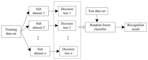
After calculating the characteristic parameters, the polarization random noise signal is recognized in the random forest. Based on bootstrap aggregation, random forest is a strong classifier that includes multiple weak classifiers (decision trees). First, put back sampling through the self-help method and set up training sub-datasets, with each set forming a decision tree. Then, randomly select characteristic parameters to train the decision trees. Each decision tree is irrelevant to the others. When making a decision, vote on the decision results made by multiple decision tree classifiers to obtain the final result (Drachenko and Mikhnyuk, 2020; Nishiyama et al., 2020). The recognition performance of random forest is higher than that of a single decision tree and overcomes the overfitting problem of decision trees. At the same time, due to random sampling, the variance of the training model is small, the generalization ability is strong and the model is robust to missing data and unbalanced data. The random forest model is shown in Fig. 3.

Figure 3 Random forest model.

The random forest algorithm here uses the method of feature selection on the basis of a Gini coefficient and classification of a regression tree and a decision tree. A Gini coefficient represents the chaotic degree of the model. A smaller Gini coefficient will lead to a smaller chaotic degree. The feature which has the smallest Gini coefficient is selected to ensure that all samples of each sub-node belong to one classification. The probability distribution's Gini coefficient is

$$\begin{array}{}\text{(14)}& \text{Gini}\left(p\right)=\mathrm{2}p(\mathrm{1}-p).\end{array}$$

In Eq. (14), Gini(p) is the Gini coefficient as a measure of the degree of chaos in a dataset. The smaller the Gini coefficient, the less chaos in the dataset, i.e. the higher the purity of the dataset. p represents the probability of a certain category appearing in the dataset. In dichotomous problems, p usually indicates the probability of a positive class and (1−p) indicates the probability of a negative class. In the multi-classification problem, the Gini coefficient is calculated separately for each category and considers the category distribution. As for sample set C, after traversing all the segmentation points of feature parameter A, it is separated into two parts by using the relationship between the feature parameter and threshold T_A (such as A > T_A), i.e. sample set C₁ satisfying A > T_A and sample set C₂ not satisfying A > T_A. In the case of A > T_A, the sample set's Gini index is

$$\begin{array}{}\text{(15)}& \text{Gini}(C,A)={\displaystyle \frac{\left|C_{\mathrm{1}}\right|}{\left|C\right|}}\text{Gini}\left(C_{\mathrm{1}}\right)+{\displaystyle \frac{\left|C_{\mathrm{2}}\right|}{\left|C\right|}}\text{Gini}\left(C_{\mathrm{2}}\right).\end{array}$$

In the equation, Gini(C₁) and Gini(C₂) represent the uncertainty of sample sets C₁ and C₂, respectively, and Gini(C,A) indicates set C's uncertainty after A > T_A division.

The cart decision tree is a binary tree. In accordance with the various numerical characteristics of the dependent variables which are in the dataset, the regression tree and classification tree can be established. The specific steps are as follows:

• 1.

  Through the self-help method, sub-datasets are obtained. Characteristic parameters randomly selected are taken as the division characteristics of the classification tree node. For each selected characteristic parameter A, take all possible thresholds T_A, calculate the sub-dataset's Gini coefficient after A > T_A division and select the characteristic parameter which has the smallest Gini coefficient as well as the corresponding threshold as the characteristic division point of the node.

• 2.

  If the node sample number or the tree depth meet the requirements, the construction of the classification tree ends and the successful cart decision tree is returned. Otherwise, step (1) is executed recursively for the two child nodes.

In this paper, the bandwidth occupied by three characteristic parameters, kurtosis and the largest normalized transient amplitude spectral density of the zero centre is used, and the polarization random noise signal is categorized and identified by a random forest classifier. First of all, normalize the signal power under various signal-to-noise ratios, extract the characteristic parameters of the noise signal and form the training dataset and test dataset of the random forest. Secondly, the training dataset is sampled by the self-help method to construct training sub-datasets. Each training sub-dataset establishes a decision tree. Characteristic parameters randomly selected are used to train the decision tree. Then, multiple irrelevant decision trees are generated, all of which form a random forest. Finally, the random forest is used to classify and identify the test dataset. The decision results are determined by the majority vote of each decision tree classifier. The obtained polarization random noise signal recognition model on the basis of the random forest is shown in Fig. 4.

Figure 4 Identification model of polarization random noise based on random forest.

2.3 Suppression of polarization random noise in a two-dimensional force sensor

The expression relationship between signal frequency f_t and time t of polarization random noise in a two-dimensional force sensor is as follows:

$$\begin{array}{}\text{(16)}& f_t=f_{\mathrm{0}}+{\displaystyle \frac{\mathrm{\Delta }V}{T_m}}t,\mathrm{0}<t<T_m.\end{array}$$

In the equation, f₀ represents the carrier frequency of the noise signal, ΔV represents the largest frequency offset and T_m represents the signal period.

The expression relationship between polarization random noise signal echo frequency f_r and time t is as follows:

$$\begin{array}{}\text{(17)}& f_{\mathrm{r}}=f_{\mathrm{0}}+{\displaystyle \frac{\mathrm{\Delta }V}{T_m}}\left(t-{\displaystyle \frac{\mathrm{2}R}{c}}\right),\mathrm{0}<t<T_m.\end{array}$$

In the equation, R represents the distance of the two-dimensional force sensor and c represents the propagation speed of the polarization random noise signal. The equation describes the relationship between the echo frequency and the time of polarized random noise signals in a two-dimensional force sensor. The echo frequency is the sum of the carrier frequency and a frequency offset that varies over time. This frequency offset is determined by the maximum frequency offset, signal period and signal propagation time. Therefore, the equation actually describes a physical process: when a polarized random noise signal propagates in a two-dimensional force sensor, its echo frequency will change over time, which is determined by the carrier frequency, maximum frequency offset, signal period and distance and speed of the signal propagation. According to the above calculation equation, the relationship between differential frequency f_i and sensor distance R can be obtained:

$$\begin{array}{}\text{(18)}& f_{\mathrm{r}}={\displaystyle \frac{\mathrm{2}\mathrm{\Delta }V}{c{T}_m}}R.\end{array}$$

Linear frequency modulation selects the best suppression position R₀ according to the difference frequency signal between the polarization random noise signal and the ordinary polarization signal. When the optimal suppression position is given, the corresponding differential frequency f_i0 can be obtained according to Eq. (19). A bandpass filter with centre frequency f_i0 is set in the two-dimensional force sensor to let the required differential frequency signal pass through and suppress signals of other frequencies.

Due to the relative motion of the polarization random signal, the calculation equation of the frequency variation Δf_i of the differential frequency signal in one modulation period T_m is

$$\begin{array}{}\text{(19)}& \mathrm{\Delta }{f}_i={\displaystyle \frac{\mathrm{2}k{v}_j{T}_m}{c}}={\displaystyle \frac{\mathrm{2}{v}_j\mathrm{\Delta }V}{c}}.\end{array}$$

In the equation, $k=\frac{\mathrm{\Delta }V}{T_m}$ represents the frequency modulation slope and v_j represents the data change speed of the two-dimensional force sensor.

In a modulation period T_m, the ratio ε which is between the frequency variation of the differential frequency signal and the frequency of the differential frequency signal is

$$\begin{array}{}\text{(20)}& \mathit{\epsilon }={\displaystyle \frac{\mathrm{\Delta }{f}_i}{f_i}}={\displaystyle \frac{T_m{v}_j}{R}}\ll \mathrm{1}.\end{array}$$

That is, if Δf_i≪f_m, the frequency f_i of the differential frequency signal in one modulation period T_m can be considered the fixed value. Therefore, the polarization random noise interference can be suppressed by fast Fourier transform. The principal block diagram of noise interference suppression is shown in Fig. 5.

Figure 5 Schematic diagram of noise interference suppression.

Because the signal in a period T_m can be considered a single frequency, its spectrum is an impulse function. The noise spectrum is uniform. Find the largest value of the polarization signal spectrum with noise interference, set it to zero and then perform fast Fourier transform to obtain noise interference. The interference noise signal is subtracted from the polarization signal containing noise interference to obtain the polarization signal after noise interference suppression.

3 Experimental verification

This article uses the simulation software MATLAB to generate a dataset and conduct a simulation experiment. The dataset to be tested contains ordinary signals and noisy signals. The signal parameters are set as follows. The symbol rate is 50 Hz. The carrier frequency is 1.55 MHz. The sampling frequency is 62 MHz. The m sequence with a period of 127 is used as the pseudo-random code sequence and the pseudo-random code rate is 635 kHz. The noise is zero mean Gaussian white noise and the signal-to-noise ratio ranges from −15 to 5 dB, with an interval of 1 dB. The training dataset and the test dataset are generated through MATLAB. Under different signal-to-noise ratio conditions, 2000 training data and 1000 test data are generated for ordinary signals and noisy signals.

3.1 Influence of the decision tree number on the performance of the method

In order to ensure that the generated random walk signals follow natural patterns in real life, in-depth research has been conducted on signals in real life to understand their statistical characteristics and variation patterns. Next, in MATLAB, these characteristics are utilized to simulate the signal, ensuring that the simulated signal is similar to the real signal in terms of amplitude, frequency and phase. In addition, the introduction of an m sequence as a pseudo-random code sequence not only increases the randomness of the signal but also makes it closer to the signal mode in actual communication. At the same time, by adding zero mean Gaussian white noise, the common noise interference in the real environment was simulated, thereby improving the fidelity of the signal. Finally, strict statistical analysis was conducted on the generated signal, which was compared with real-life signals to ensure that the statistical characteristics of the simulated signal were consistent with the real signal. These measures collectively ensure that the random walk signals generated in the experiment closely follow the natural patterns in real life. The comparison between the random walk signals generated by the research plan and the signals generated by non-random processes is shown in Fig. 6.

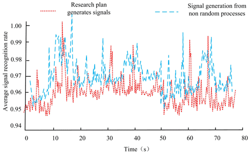
Figure 6 Comparison of signals between random walk signals generated by the research plan and data generated by non-random processes.

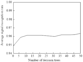
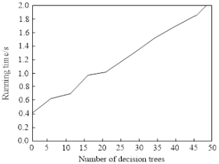
From Fig. 6, it can be seen that the random walk signals generated by the research scheme exhibit a high degree of similarity to the signals generated by non-random processes. The decision tree number is taken from 1 to 50 at an interval of 5. The average recognition rate of all the test data in the whole test set of this method is shown in Fig. 7 and the running time is shown in Fig. 8.

Figure 7 Average recognition rate of the signals.

Figure 8 Running time.

By analysing Fig. 7 in depth, it can be clearly observed that there is a positive correlation between the average correct recognition rate of the signal and the number of decision trees. The figure clearly shows that, as the number of decision trees gradually increases, the average correct recognition rate of the signal also improves accordingly. This trend indicates that the integration of multiple decision trees helps improve the accuracy of the signal recognition. However, it is worth noting that when the number of decision trees exceeds 10, the growth trend of the recognition rate begins to stabilize, which means that further increasing the number of decision trees may not bring a significant improvement in the recognition rate. Meanwhile, another important factor to consider is the running time. The data in Fig. 8 show that the more decision trees there are, the longer the required running time will be. This is clearly a balancing issue, as although adding decision trees can improve recognition rates, it will also sacrifice operational efficiency. After considering both the recognition rate and the running time, the study selected 10 decision trees as the optimal balance point in the simulation experiment. This choice aims to ensure a high recognition rate while also controlling the running time, thereby achieving overall optimization of the performance of the method.

3.2 Comparison of the correct signal recognition rates

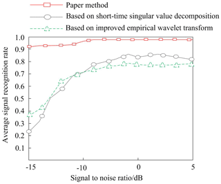
When the signal-to-noise ratio range was −15 to 5 dB, this method was compared with noise suppression methods based on short-time singular-value decomposition and improved empirical wavelet transform. Ensuring the improvement of the signal quality is crucial in signal conversion pipelines. In this process, adaptive filtering technology is first adopted to effectively remove noise components from the original signal and improve the signal-to-noise ratio of the signal. Then, through normalization processing, the signal is scaled to a unified scale and signal features are extracted using time domain analysis, frequency domain analysis or time–frequency domain analysis techniques. Use short-time Fourier transform (STFT) or wavelet transform to obtain the time–frequency characteristics of the signal. Transform the extracted features into a matrix data structure suitable for model processing. The comparison results of signal recognition accuracy are shown in Fig. 9.

Figure 9 Comparison results of the correct signal recognition rate.

According to the experimental results shown in Fig. 9, it can be clearly seen that the proposed method exhibits an excellent polarization random noise signal recognition ability in an environment with a signal-to-noise ratio range of −15 to 5 dB. This innovative method has a relatively high accuracy in identifying polarization random noise signals generated by two-dimensional force sensors. Compared with the two commonly used traditional methods, this method has significant advantages in the signal recognition rate. The data show that its average signal recognition rate is not only higher than these two traditional methods but also reaches an astonishing recognition rate of 0.99 under certain conditions. This achievement undoubtedly proves the effectiveness and superiority of the research method in identifying noise signals, providing a new solution to the noise suppression problem of two-dimensional force sensors.

3.3 Noise suppression effect

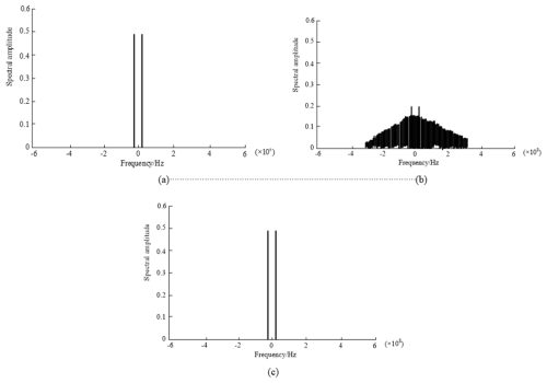
As the key performance of the method of noise suppression, the noise suppression effect can fully reflect the suppression performance of the method. Therefore, the polarization random noise suppression effect of the method in this paper is verified based on the noise-free polarization random noise signal spectrum and by adding a signal-to-jamming ratio (SJR) = −10 dB interference noise to the basic signal to inspect the noise suppression effect.

The results in Fig. 10 show that the method in this paper has a good noise suppression effect and can remove the interference noise in the signal, and the signal after noise suppression is basically suppressed from the original signal.

Figure 10 Noise suppression effect. (a) Signal spectrum without interference noise. (b) Noise-containing interference signal spectrum when SJR = −10 dB. (c) Signal spectrum after noise suppression.

3.4 Noise suppression efficiency

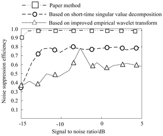
Due to the high workload of a two-dimensional force sensor and the large amount of data to be collected and processed, efficiency of the method of noise suppression is required. Therefore, it is necessary to compare and verify the noise suppression efficiency of this method. To further enhance the generalization ability of the model, the L1 and L2 regularization techniques were used. L1 regularization helps to generate a sparse-weight matrix, remove noise and perform feature selection. L2 regularization smoothens the weights and prevents the model from overfitting. Meanwhile, using the dropout technique, some of the neurons were randomly discarded during training to reduce the dependence of the model on the training data.

Analysing the comparison results of the noise suppression efficiency shown in Fig. 11, it can be seen that this article has high noise suppression efficiency and good noise suppression stability, which can ensure the stability of the two-dimensional force sensor operation and improve the reliability of the data transmission.

Figure 11 Noise suppression efficiency.

4 Conclusion

To improve the data transmission quality of a two-dimensional force sensor, a polarization random method of noise suppression in a two-dimensional force sensor based on random forest is proposed. The performance of the method is verified theoretically and experimentally. This method has a higher correct recognition rate of noise signals and a better noise suppression efficiency when suppressing polarization random noise in a two-dimensional force sensor. Compared with the method in terms of short-time singular-value decomposition and an improved empirical wavelet transform, the correct recognition rate of noise signals using this method is significantly improved and finally stabilized at 0.99. Moreover, the noise suppression effect of this method is good and the data after noise suppression are basically consistent with the original data. Therefore, the proposed method of noise suppression based on random forest can better meet the requirements of polarization random noise suppression in a two-dimensional force sensor.