Flow measurement by means of wideband acoustic signals in single-mode waveguides

A novel concept of an acoustic flowmeter, based on single-mode waveguides, is proposed, implemented, and analysed in this work. Instead of transmitting a pulse diagonally across the duct's cross-section, this device operates with two ducts that operate simultaneously as pipes and as waveguides. Below the frequency threshold for single-mode propagation, acoustic waves are forced to traverse the waveguides with a plane front, precluding the possibility of beam drifting, inner reflections, and spreading losses. This enables the designer to flexibly increase the sound path and perform a highly sensitive measurement of the flow velocity and speed of sound, even if the excitation frequency is required to be kept below a relatively low value. A device based on this principle was constructed and tested for flow measurements in air. It consists of two waveguides of a circular cross-section (5 mm diameter) coupled to electroacoustic transducers for the transmission of a wideband chirp (9.8–18.2 kHz). Usage of a wideband signal was possible due to the combined frequency response of a special kind of micromachined ultrasound transducer (MUT) and a commercial micro-electromechanical system (MEMS) microphone. The constructed flowmeter was capable of measuring flow velocities up until the transition to turbulent flow at 16 L min⁻¹ with a resolution of 0.3 L min⁻¹, and it also detected changes of less than 0.2 m s⁻¹ in the speed of sound. This topology for flow measurement could prove advantageous for applications where gases of variable composition are conducted in ducts of diameters in the millimetre range.

1 Introduction

Acoustic signals have been widely used to measure flow in pipes, without requiring interaction of the fluid with mechanical parts or bringing about a significant head loss. In the classical configuration, two ultrasonic transducers are arranged diagonally to transmit pulses across the pipe's cross-section such that their transit time in the upstream and downstream directions may be used to calculate the flow velocity and speed of sound (Köchner et al., 1996). This arrangement compels the designer to seek a transducer with a high operation frequency in order to achieve a high resolution and a focused beam emission. Although effective, this method is limited by beam drift and signal attenuation, particularly in applications with small duct diameters. The case of beam drift is illustrated in Fig. 1a, where the flow velocity is such that the emitted pulse does not reach the receiver. This limitation may be overcome with the introduction of reflectors (von Jena et al., 1993) or, more elegantly, with the usage of a multi-mode waveguide within the pipe, as disclosed by Mueller et al. (2014) – see Fig. 1b. With a multi-mode waveguide, the sound energy is distributed along multiple propagation paths, each undergoing a different number of reflections so that the acoustic signal may be transmitted in spite of high flow velocities that cause significant beam drift. Nonetheless, beam drift can be excluded altogether by turning the pipe itself into a single-mode waveguide, as proposed in Fig. 1c.

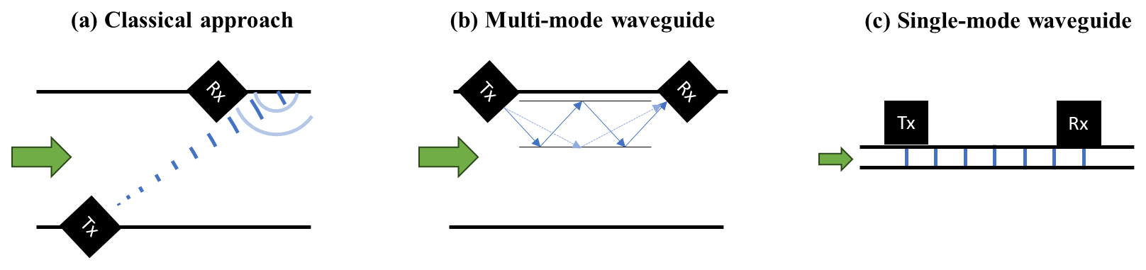
Figure 1 Schemes of alternative strategies to measure flow with acoustic signals. (a) Classical approach where the transmitter (Tx) and receiver (Rx) are arranged diagonally (see, for instance, Köchner et al., 1996). (b) Multi-mode waveguide approach disclosed by Mueller et al. (2014). (c) Single-mode waveguide approach introduced in this work.

In a single-mode waveguide, the acoustic excitation travels as a longitudinal wave along the duct without inner reflections – even if the duct does not follow a straight line. This is only possible if the excitation frequency is kept below a certain threshold such that the wavelength is too large to allow the formation of standing waves in the duct's cross-section (Trusler, 1991). The solution of the two-dimensional wave equation in an enclosed surface yields discrete solutions, the first of which is the trivial case of a constant pressure, followed by more complex pressure profiles – i.e. higher modes – that are only allowed above a certain frequency. If a pressure excitation enters a waveguide, its energy will be distributed into the allowed propagation modes; therefore, at low enough frequencies, only the first propagation mode will be activated. The reader is encouraged to observe this phenomenon of single-mode propagation in the measurements of Meykens et al. (1999) in a rectangular waveguide. A transmission of acoustic signals that is independent of the directivity of the transducer is also beneficial for applications where the gas composition changes, one practical case being the mixture of natural gas and hydrogen (Melaina et al., 2013). Even if a transducer is optimised to emit a focused beam through natural gas, the significantly lower density of hydrogen may cause the directivity pattern to transition towards an omnidirectional one, provoking undesired reflections that distort the signal. This effect would also be precluded if a single-mode waveguide is utilised.

A further advantage of single-mode waveguides concerns signal attenuation. In the classical arrangement, the wavelength of the pulse is expected to be much smaller than the diameter of the pipe, which results in a spherical wavefront that entails an amplitude loss inversely proportional to the travelled distance – even if there were no energy losses. On the other hand, the wavefront in a single-mode waveguide is forced to remain planar, thus excluding any sort of spreading losses. A further source of amplitude reduction is given by absorption. Energy absorption within the fluid brings about an exponential decay in the signal that is further multiplied by the spreading loss (Hutchins and Neild, 2012; Dahl et al. 2014). If the diagonal arrangement is to be used in a pipe of small dimensions (e.g. millimetre range), the excitation frequency ought to be increased correspondingly (e.g. MHz range), but at high frequencies the energy loss mechanisms of the gas become increasingly relevant – consider the case of “classical absorption”, for example, which increases quadratically with frequency (Trusler, 1991). If, instead, frequency is reduced below the threshold for single-mode propagation, absorption losses may be kept to a negligible amount. Nonetheless, absorption may become relevant in ducts of a very small diameter (e.g. sub-millimetre range) if this dimension becomes comparable to the thermal or viscous boundary layers, whose impact can only be ignored if the duct's smallest dimension is much larger than them.

In this work, we propose and test the concept of an acoustic flowmeter based on single-mode waveguides. Despite requiring operation at lower frequencies than the classical arrangement, this device may achieve a high resolution because its sound path (i.e. the distance between the transmitter and receiver) may be increased freely without concerns regarding beam drift or signal attenuation. Clearly, a large sound path implies a less compact device, but the overall size can be reduced by bending the duct without the risk of provoking reflections. An upper limit to the flow velocity that this system can measure is nevertheless expected after flow transitions from laminar to turbulent, which may cause significant distortions on the acoustic signals. Although this flowmeter concept could be applied to both liquids and gases, our implementation is indeed focused on gases. We aim thus to demonstrate the single-mode functioning principle and assess the capabilities of such a device to measure both speed of sound and flow velocity.

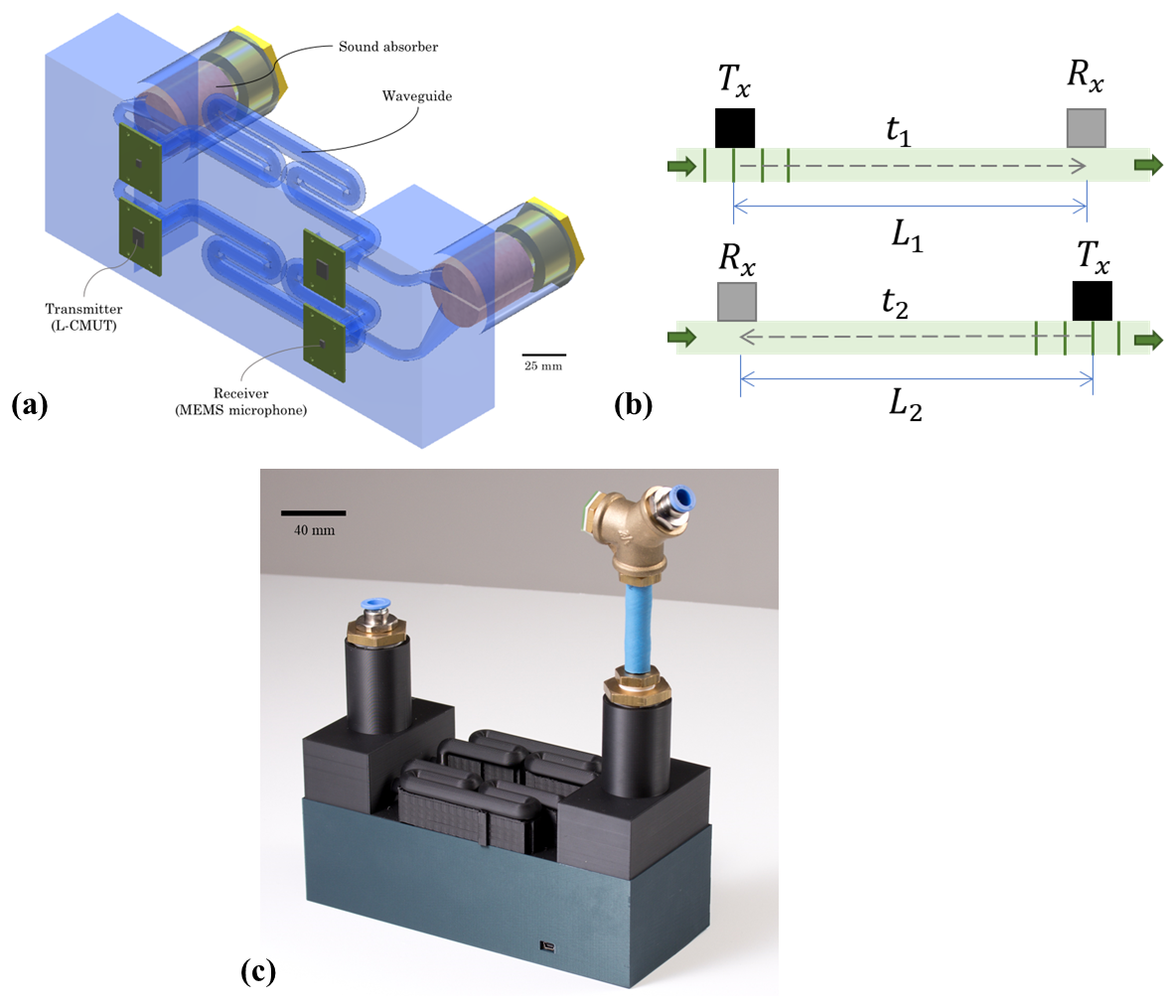
Figure 2 Depiction of a prototype single-mode waveguide flowmeter. (a) Accurate illustration of the fabricated prototype. (b) Simplified schematic of the waveguides, indicating the definition of the sound paths (L₁ and L₂) and the corresponding transit times (t₁ and t₂). (c) Photograph of the fabricated device, including the temperature and pressure sensors at the inlet. A gas is introduced at one of the ports and distributed equally into two branches that act as acoustic waveguides. Electroacoustic transducers are placed at opposite ends of each waveguide to measure the transit time of ultrasound both with the flow and against it.

2 System description

We constructed a waveguide flowmeter according to the schematic in Fig. 2. The device consists of two waveguides, each of which is coupled to an ultrasonic transmitter and a microphone at opposite ends. The housing that contains the waveguides was fabricated by fused deposition modelling. The gas is introduced into the housing via a G-$\mathrm{1}/\mathrm{2}$ fitting and split into two identical branches that act as acoustic waveguides of a circular cross-section (5 mm inner diameter). These branches are then joined together at the gas outlet. The purpose of these two branches is to split the flow into equal proportions and perform measurements in both directions: one where sound travels with the flow and one where it travels against it. Each branch is therefore coupled to an electroacoustic transmitter at one end and to a receiver at the opposite end. Given that sound is not only directed towards the waveguide but also diverted towards the gas inlet and outlet, sound absorbers (Basotect^® foam) were introduced to suppress acoustic interferences between the two waveguides. The diameter of 5 mm yields a threshold of 40 kHz for single-mode propagation in air (assuming a speed of sound of 343 m s⁻¹), which corresponds to a ratio between the diameter and wavelength of less than ∼ 0.586 (Trusler, 1991). These waveguides were purposely bent several times (radius of 6 mm) to reduce the overall size of the prototype and to verify the absence of inner reflections according to the theory. The design length of the waveguides is 354 mm, so the transit time is expected to be close to 1 ms. We further implemented temperature (Texas Instruments^® TMP117) and pressure sensors (STMicroelectronics^® ILPS28QSW) at the inlet of the system (see Fig. 2c). We used a microcontroller (STMicroelectronics^® ILPS28QSW) to generate and capture the signals of the transmitters and receivers with a sampling rate of 2 MHz.

Two different kinds of electrostatic micro-electromechanical system (MEMS) transducers were implemented for the transmission and reception of acoustic waves. The transmitter is a special kind of capacitive micromachined ultrasonic transducer (CMUT), which operates with laterally oscillating microbeams instead of vertically vibrating membranes. We thus denote it as “L-CMUT” (Monsalve et al., 2022). This L-CMUT has a relatively low Q factor that, despite dampening the response near its natural frequency, grants it a relatively large bandwidth. Its undamped eigenfrequency is expected at 50 kHz and its Q factor around 1.0, although deviations due to the manufacturing process may have taken place. The receiver, on the other hand, is a commercial MEMS microphone (Knowles^® SPH18C3LM4H-1), based on the classic membrane principle, whose natural frequency is expected at 40 kHz according to the fabricant. These electroacoustic devices may, at first glance, be understood as mechanical resonators, but it is important to note that they are subject to additional effects. The L-CMUT, being a nonlinear transducer governed by a Coulomb force, emits pulses with a certain distortion in the second harmonic. Hence, even if the threshold for single-mode operation of the waveguide is expected at 40 kHz, the presence of a second harmonic implies that the higher propagation modes may be activated when the L-CMUT is excited near 20 kHz. In addition, trials with the MEMS microphone revealed that, apart from the nominal resonance at 40 kHz, further peaks in its frequency response were observed between 30 and 50 kHz, as shown in more detail in the upcoming results.

Coupling these two transducers enables the transmission of wideband signals, which offer the possibility of a more accurate and robust time-delay estimation than single-frequency pulses through a calculation of the cross-correlation integral (Silvia, 1987; Weinstein and Weiss, 1984). The peak of the cross-correlation is an accurate estimator of the time shift between two signals that are otherwise identical (or scaled in amplitude). Pulses with a longer duration and a wider frequency content result in a sharper and higher peak of this integral, yielding higher accuracy in the estimation of the time delay. Moreover, the requirement for a minimum signal-to-noise ratio for accurate peak detection is reduced in signals with a wider frequency content, making the time-delay estimation more robust than in the narrowband case (Weinstein and Weiss, 1984).

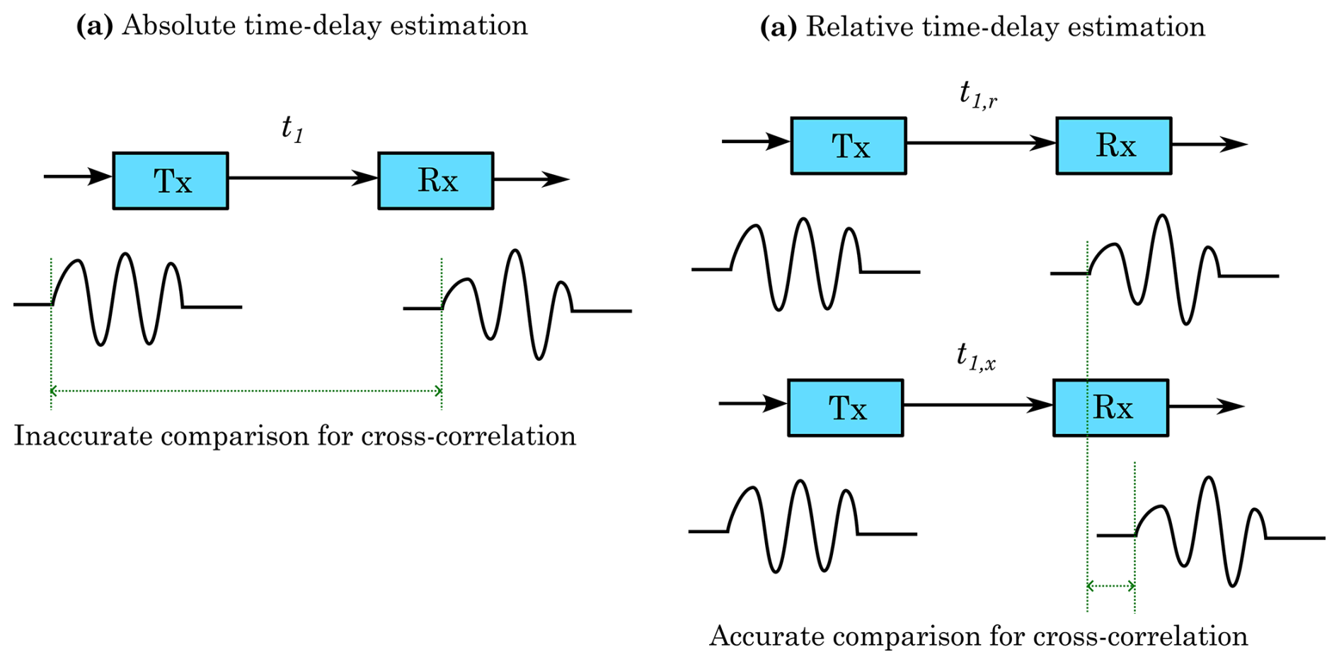
Figure 3 Illustration of the proposed method to increase the accuracy of the time-delay estimation by performing a relative comparison to a calibration measurement. (a) Direct calculation of the cross-correlation integral between the sent and received signal, suffering from inaccuracies because of the filtering effect of both the transmitter and the receiver on the measured signal. (b) Relative calculation of the cross-correlation integral between an arbitrary measurement and a reference measurement, whose signals can be more accurately compared as time-shifted versions of one another.

2.1 Calculation of the speed of sound and flow velocity

The classical method to calculate the flow velocity and speed of sound is based on the direct measurement of the travelling time of acoustic waves (Köchner et al., 1996); nevertheless; here we depart from this paradigm towards a relative time-delay estimation with respect to a reference signal, as this was proven to yield more accurate measurements. Our proposed methodology is illustrated in Fig. 3. If the time delay between the moment the signals are triggered and the moment they reach the receivers is measured (t₁ for path “1” and t₂ for path “2”), the calculation of the speed of sound (c) and flow velocity (v) is straightforward, as shown in Eqs. (1) and (2). The sound paths of each waveguide (L₁ and L₂) need not be identical, so they are left as independent variables. The estimation of this time delay requires comparing the sent signal against the received signal, but these two are not simply scaled and time-shifted versions of one another. This is due to the filtering effect of both the transmitter and the receiver on the signal, altering its final shape with respect to the computer-generated chirp. This may lead to inaccuracies in the position of the peak of the cross-correlation.

$$\begin{array}{}\text{(1)}& {\displaystyle }& {\displaystyle }\mathrm{2}c={\displaystyle \frac{L_{\mathrm{1}}}{t_{\mathrm{1}}}}+{\displaystyle \frac{L_{\mathrm{2}}}{t_{\mathrm{2}}}}\text{(2)}& {\displaystyle }& {\displaystyle }\mathrm{2}v={\displaystyle \frac{L_{\mathrm{1}}}{t_{\mathrm{1}}}}-{\displaystyle \frac{L_{\mathrm{2}}}{t_{\mathrm{2}}}}\end{array}$$

Instead of comparing the received signal against the sent signal, we compute the relative time shift between two received signals: an initial one used for calibration (for instance, without flow) and a later one obtained at the desired measurement. These two received signals are nearly identical in shape, so the cross-correlation between them offers a very accurate estimation of the relative time shift. The estimation of the travelling time of the calibration signal is still necessary to compute the sound paths of both waveguides, but it is performed only once. With this alternative strategy, the measured variables are not the transit times (t₁ and t₂) but the difference in the transit times with respect to those of the reference signals (Δt₁ and Δt₂). These transit time differences can be expressed as a function of the respective speeds of sound (at the reference condition, c_r, and during the measurement, c_x) and flow velocities (v_r and v_x) according to Eqs. (3) and (4).

$$\begin{array}{}\text{(3)}& {\displaystyle }& {\displaystyle }\mathrm{\Delta }{t}_{\mathrm{1}}={\displaystyle \frac{L_{\mathrm{1}}}{c_x+v_x}}-{\displaystyle \frac{L_{\mathrm{1}}}{c_{\mathrm{r}}+v_{\mathrm{r}}}}\text{(4)}& {\displaystyle }& {\displaystyle }\mathrm{\Delta }{t}_{\mathrm{2}}={\displaystyle \frac{L_{\mathrm{2}}}{c_x-v_x}}-{\displaystyle \frac{L_{\mathrm{2}}}{c_{\mathrm{r}}-v_{\mathrm{r}}}}\end{array}$$

Therefore, the speed of sound and flow velocity can be solved as follows:

$$\begin{array}{}\text{(5)}& {\displaystyle }& {\displaystyle }\mathrm{2}{c}_x={\displaystyle \frac{L_{\mathrm{1}}}{\mathrm{\Delta }{t}_{\mathrm{1}}+\frac{L_{\mathrm{1}}}{c_{\mathrm{r}}+v_{\mathrm{r}}}}}+{\displaystyle \frac{L_{\mathrm{2}}}{\mathrm{\Delta }{t}_{\mathrm{2}}+\frac{L_{\mathrm{2}}}{c_{\mathrm{r}}-v_{\mathrm{r}}}}},\text{(6)}& {\displaystyle }& {\displaystyle }\mathrm{2}{v}_x={\displaystyle \frac{L_{\mathrm{1}}}{\mathrm{\Delta }{t}_{\mathrm{1}}+\frac{L_{\mathrm{1}}}{c_{\mathrm{r}}+v_{\mathrm{r}}}}}-{\displaystyle \frac{L_{\mathrm{2}}}{\mathrm{\Delta }{t}_{\mathrm{2}}+\frac{L_{\mathrm{2}}}{c_{\mathrm{r}}-v_{\mathrm{r}}}}}.\end{array}$$

In order to increase the sensitivity of the time-delay estimation, peak detection with quadratic interpolation was performed on the cross-correlation. In other words, three points of the curve (maximum and two immediate neighbours) were taken to fit a parabola and thus interpolate the most likely location of the maximum with an accuracy beyond the sampling period. Although this improves the calculation of the “best estimate” of the transit time, its experimental uncertainty still ought to be regarded as half of the sampling period. This uncertainty is then propagated to estimate the error of the flow velocity and speed of sound by performing the corresponding partial derivatives in Eqs. (5) and (6). (See Taylor, 1997, for more details on the procedure for error propagation.)

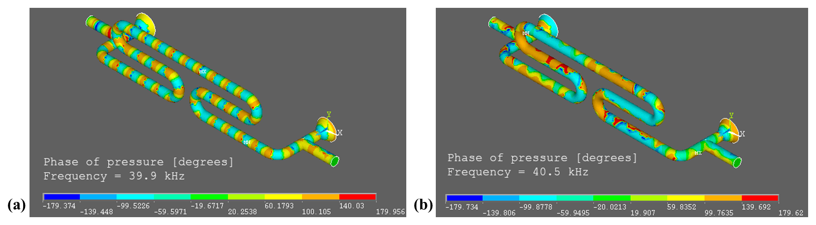
Figure 4 Transition of the steady-state propagation of ultrasound in the modelled waveguide as observed in the phase of the nodal pressure. (a) Phase of pressure slightly below the cutoff frequency (40 kHz), showing single-mode plane-wave propagation. (b) Phase of pressure slightly above the cutoff frequency, showing that a further mode has been activated and that a plane-wave front is no longer kept.

2.2 Simulation of wave propagation

With the aid of a finite-element model, it can be verified whether the expected plane-wave propagation below 40 kHz, even despite the curved shape of the waveguide, is to be expected. A three-dimensional model of the waveguide was constructed in ANSYS APDL (2023 R1), applying a mesh of FLUID220 elements (Helmholtz equation) of a size smaller than 0.9 mm (which corresponds to $\mathit{\lambda }/\mathrm{6}$ at 60 kHz). This geometry can be visualised in Fig. 4. The two cones at opposite ends of the waveguide are the acoustic ports where either the transmitter or the receiver is coupled. Next to these ports are the T sections where the gas is introduced into or led out of the waveguide. A certain measure of the acoustic excitation is expected to divert through these sections, so an absorbing layer (PML) was attached at their ends to account for this loss. Elsewhere, the boundary condition was left as the default Neumann one (sound hard) to account for the rigid walls. A constant surface velocity of 0.1 mm s⁻¹ was applied at one of the acoustic ports, and the nodal pressure was simulated in the frequency domain from 2 to 60 kHz. The plots in Fig. 4 show the radical transition in the progression of waves from 39.9 to 40.5 kHz. Slightly below 40 kHz, the phase of the nodal pressure appears as a sequence of rings following the path of the acoustic wave; that is, pressure waves do traverse the channel (including the bent sections) as a longitudinal wave. However, slightly above 40 kHz, the phase plot bears no resemblance to the previous case, indicating that the next higher propagation mode was activated.

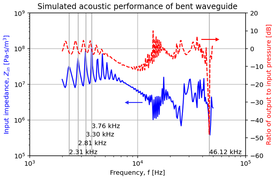
Figure 5 Simulated acoustic impedance at the input port and ratio of output to input pressure amplitude.

It is also instructive to observe the evolution of the acoustic impedance (ratio between pressure and volume velocity) at the input port, as well as the ratio of pressure at the output port with respect to the input port, shown in Fig. 5. The input impedance exhibits a series of peaks at low frequencies, which resemble a resonance pattern. This is not surprising, given that in a steady-state excitation the waves could be reflected back and forth between the input and output ports (although a portion of the waves is diverted at the T sections). If a standing wave is formed along the length of the waveguide, these peaks should correspond to an integer ratio between the sound path and $\mathit{\lambda }/\mathrm{2}$. Indeed, one can verify that the marked peaks match a sequence of 5, 6, 7, and 8 times $\mathit{\lambda }/\mathrm{2}$ for a length of approximately 0.36 m. These peaks are also observed in the ratio of input and output pressures. This ratio tends to oscillate near 0 dB at low frequencies, descending to near −10 dB around 8 kHz and then returning to 0 dB. It is noticeable that the output pressure is simulated to vanish at 46 kHz, where the acoustic excitation is fully lost at the T sections.

3 Characterisation

3.1 Acoustic behaviour

In order to select an appropriate frequency band for transmitting a wave packet, it is useful to measure the steady-state frequency response of the transmitter–channel–receiver system. It is desirable to find a range with a nearly flat transfer function (to reduce amplitude modulations), with the highest possible centre frequency (to increase resolution), and yet also unaffected by distortions caused by higher transmission modes. The frequency-dependent output of the receivers upon a constant-amplitude excitation of the transmitters (10 V amplitude, 30 V bias) was measured with an audio analyser (NTI Flexus FX 100) in the range of 800 to 80 kHz. In a further measurement, the receiver was replaced by a calibrated microphone (Microtech Gefell, MK 301E, $\mathrm{1}/\mathrm{4}$ in.) to obtain the actual acoustic pressure at the end of the waveguide and distinguish the influence of the receiver's own frequency response.

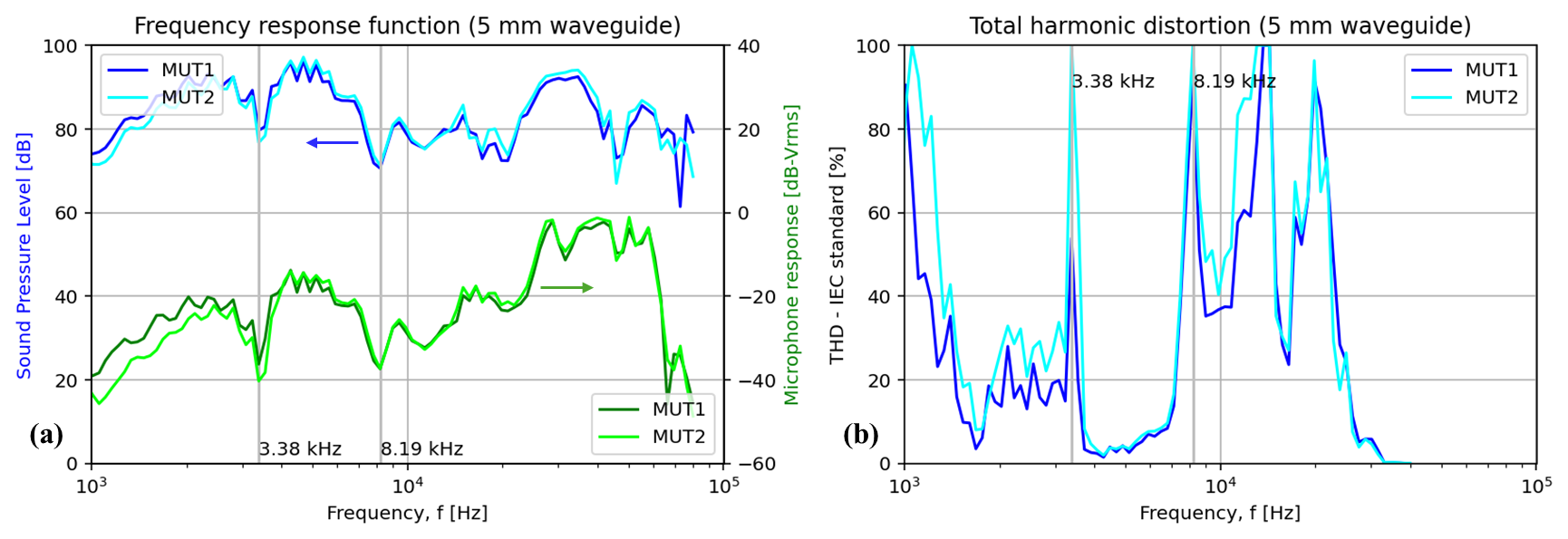
Figure 6 Steady-state frequency responses of the two pairs of transmitter–receiver systems, corresponding to each branch of the flowmeter. (a) Measurement of pressure at the output ports of the waveguides, both as measured by a calibrated microphone (in dB relative to 20 µPa-rms) and as recorded by the MEMS microphones (in dB-Vrms) used as receivers. (b) Corresponding plot of the total harmonic distortion (IEC standard) of the signals recorded by the MEMS microphones.

Figure 6 shows the measured steady-state frequency response of the waveguide, namely the pressure output (Fig. 6a) and the harmonic distortion (Fig. 6b). The ripples that were obtained in the simulation, corresponding to a resonance pattern, can also be observed in the measurement of pressure at low frequencies. The peaks at 2.4 and 3.2 kHz are relatively close to the respective peaks in the impedance simulation, and the peak at 2.8 kHz is matched in both curves. Nonetheless, the notches at 3.4 and 8.2 kHz were not predicted by the simulation. These minima in the pressure measurement correspond, interestingly, to peaks in the harmonic distortion. The region between these two frequencies is one where both a low signal distortion and a high sound pressure level (SPL) are observed, which makes it an interesting possibility for emitting a chirp. A further possibility would be the range above 8 kHz until about 20 kHz. Even though the simulation predicts that the cutoff frequency is rightly expected at 40 kHz, a significant amount of distortion was measured for frequencies above 8 kHz. This opens the possibility for higher modes to be excited at frequencies below 40 kHz (for instance, at 20 kHz due to the second harmonic). From 30 kHz onwards, there is a significant decrease in the distortion, as well as a mismatch between the measurement from the calibrated microphone and that from the MEMS microphones. This is an indication that the signal is heavily dominated by the microphone's own dynamic response at these higher frequencies. After a series of trials, the range between 9.8 and 18.2 kHz was found to offer a good trade-off between signal amplitude and distortion.

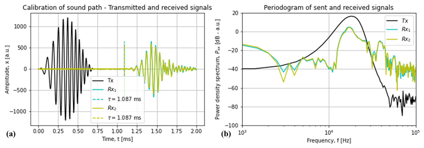
Figure 7 Readings of the microphones at both branches of the flowmeter at 0 L min⁻¹, having excited the transmitters with a linear chirp between 9.8–18.2 kHz with a Hann window. (a) Plot in the time domain marking the estimated time of arrival of the wave packets according to the cross-correlation integral. (b) Plot in the frequency domain (periodogram) of the sent and received signals.

3.2 Operation as a flowmeter

Having performed an acoustic characterisation, the L-CMUTs and MEMS microphones were connected to a microcontroller (STM32L476RG) and a self-developed circuit board with a custom amplifier and voltage supply. The system was set up to record signals in intervals of 2 ms with a sampling frequency of 2 MHz. Figure 7 shows the recording of the transmitted and received signals, both in the time domain and in the frequency domain. The time-domain plot reveals how the recorded signals nearly follow the shape of the transmitted chirp (9.8–18.2 kHz with Hann window), save for some distortions at the trailing edge. These distortions could be the result of a slower, higher mode of the waveguide that is excited due to a higher harmonic. The corresponding plot in the frequency domain (Fig. 7b) reveals that the received signals mostly follow the spectrum of the sent signal within the frequency band of the chirp, but a small peak near 40 kHz that was not present in the sent signal was indeed present in the reading of the microphones. Nonetheless, the presence of this distortion at the trailing edge did not affect the calculation of the time delay by cross-correlation. The modulation of both frequency and amplitude enabled accurate detection of the time of arrival of the wave packet. With the measured temperature of 22.9 °C and assuming a molar mass of air of 28.96 g mol⁻¹ (The Engineering Toolbox, 2004) – whilst ignoring the effect of relative humidity – we estimate that the speed of sound during the calibration measurement was 344 m s⁻¹, so the delay of 1.09 ms in both branches yields a sound path of 366 mm. This preliminary calibration, though perhaps not highly accurate from a metrology viewpoint, serves to verify the sensitivity of the device and the maximum flow that it can measure.

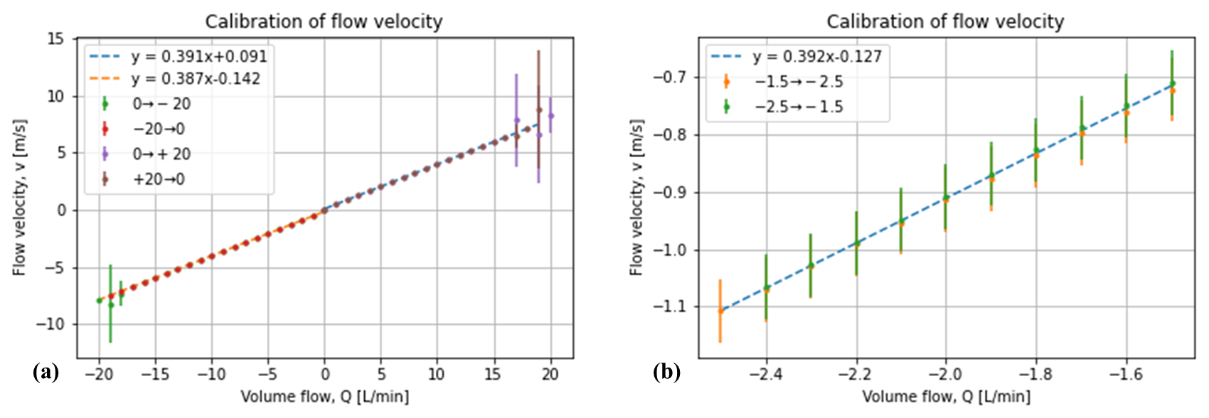
Figure 8 Correlation of the measured flow velocity and the configured volume flow in two distinct ranges. (a) Measurement from 0 to ± 20 L min⁻¹, in both increasing and decreasing steps and both feeding the gas into the inlet and the outlet. (b) Measurement around −2 L min⁻¹ in steps of 0.1 L min⁻¹ to estimate the resolution of the flowmeter.

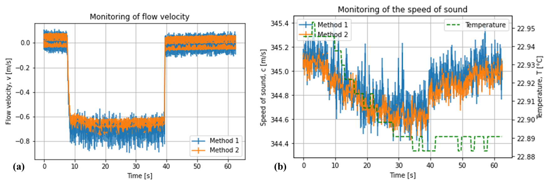
Figure 9 Continuous monitoring of (a) the flow velocity and (b) speed of sound for an experiment where a sudden flow was introduced into the device from a source of compressed air and then interrupted. Two evaluation methods are compared. Method 1 is the direct correlation between the transmitted and received signal; method 2 is the correlation between the received signal and a reference signal from a calibration measurement.

A mass flow controller (Bronkhorst^® EL-FLOW Select) was then used to introduce controlled flow of air into the waveguide flowmeter. In a first experiment, air was introduced at the inlet, and flow was varied from 0 to 20 L min⁻¹, first in increasing steps and then in decreasing steps back to 0 L min⁻¹, in order to detect any possible hysteresis. The flow was then introduced into the outlet, and the experiment was repeated to detect any possible asymmetry in the construction. At least 10 measurements were performed for each flow configuration. The results, revealed in Fig. 8a, show neither hysteresis nor asymmetry. The readings of flow velocity and the regulated volume flow follow a linear pattern with a slope that is nearly identical in both the “positive” and the “negative” flow measurements. This slope of 0.39 (m $/$ s) $/$ (L $/$ min) is equivalent to a cross-section of 21.4 mm² per waveguide (considering that flow is equally split between the two branches), which corresponds to a diameter of 5.2 mm – rather close to the design value of 5.0 mm. The linear regressions also report an intercept with a positive value for positive flows and a negative value for negative flows. This nonlinear behaviour around 0 L min⁻¹ (similar to the backlash effect in gears) is very likely due to the sound absorbers, which not only attenuate sound but also possibly oppose the flow until a certain threshold is reached. Values beyond ± 16 L min⁻¹ were excluded from the regression, as they were subject to higher errors due to noise. At these high flow rates, the passage of air itself emits a sound at low frequencies that is detected by the microphones and leads to clipping of the signal. A closer inspection reveals that this upper limit of 16 L min⁻¹ also corresponds to the critical Reynolds number of 2300 for a diameter of 5 mm. A second experiment was performed around −2 L min⁻¹, varying the flow in steps of 0.1 L min⁻¹ in order to estimate the resolution of the device. These steps of 0.1 L min⁻¹ are still above the precision of ± 5 mL min⁻¹ within which flow can be regulated with the controller. The results, presented in Fig. 8b, show a consistent slope with the wide-range measurement and a linear behaviour without hysteresis. Even though the reported values of flow velocity do increase sequentially within the steps of 0.1 L min⁻¹, the uncertainty bars (calculated according to the sampling rate) stop overlapping after a difference of ∼ 0.3 L min⁻¹.

Besides the measurement of flow velocity, it is also relevant to verify whether slight changes in the speed of sound can be detected by the device. A further experiment was conducted, where air inside the device was in equilibrium with the surroundings. Afterwards, flow from pressurised air was suddenly introduced and maintained for a certain amount of time. This flow was then abruptly interrupted so that the air from the surroundings entered the device again. The acoustic signals were recorded continuously at intervals of ∼ 0.16 s, and both the speed of sound and the flow velocity were calculated according to two methods. The first method is the direct cross-correlation between the transmitted and received signals, following Eqs. (1) and (2); the second method is the cross-correlation between the received signals and the previously recorded signals in the calibration measurement (Fig. 7). The results can be found in Fig. 9. The introduction of air from the pressurised source slowly reduced the speed of sound as the device was continuously exposed to it. Although a slight decrease in temperature of about 0.05 °C is reported, this is likely a spurious reading since the resolution of the sensor is 0.1 °C, and even if such a temperature decrease took place, it would not be sufficient to cause the decrease of 0.5 m s⁻¹. The decrease in the speed of sound was most likely caused by the source of air being not only slightly cooler but also drier than the atmospheric air. Once flow was interrupted, the speed of sound slowly increased towards its initial value, as air from the surroundings entered the device again. A rise in temperature was not measured, possibly because the sensor was placed at the port that was connected to the source. The stepwise introduction and withdrawal of air can be clearly observed in the measurement of the flow velocity. Comparison of the curves obtained by both evaluation methods (in both the speed of sound and the flow velocity) shows that the relative cross-correlation against the calibration signal (labelled as “method 2”) behaves more stably and yields a lower uncertainty than the direct cross-correlation against the sent signal. Notice, too, that no shift is observed between both curves or diverging patterns, which means that both evaluation methods are consistent with one another.

4 Conclusion

A novel method to measure flow with ultrasonic transducers, not based on the transmission of waves across the cross-section of the duct but rather along its length, was effectively implemented. By operating the transducers below a critical frequency, the duct itself performs as a single-mode waveguide where a wideband signal can be transmitted along large distances without spreading losses and internal reflections, obtaining an accurate estimation of the transit time via cross-correlation. This method is not subject to the drawbacks of beam drifting and multi-path reflections present in other acoustic flowmeters. The implemented waveguide flowmeter, coupled to a wideband MUT and a commercial MEMS microphone, was capable of detecting changes below 0.3 L min⁻¹ in a range up to 16 L min⁻¹ bidirectionally, as well as fluctuations in the speed of sound below 0.2 m s⁻¹. It exhibited a linear behaviour and no hysteresis. The range of the device was limited by noise related to the transition to turbulent flow, whereas its resolution was limited by the sampling rate of the microcontroller. The wideband characteristic of the transmitted signals enabled a robust estimation of the time delay, particularly by comparing the readings of the microphones against an initial reference signal instead of performing a direct comparison against the sent signal. This new concept may open opportunities for the development of gas counters, spirometers, and anemometers without mechanical parts, achieving a high resolution in the measurement of not only the flow velocity, but also the speed of sound, which can be used to diagnose alterations in the medium.