Detection of plastics in water based on their fluorescence behavior

Plastic waste is one of the biggest growing factors contributing to environmental pollution. So far there has been no established method to detect and identify plastics in environmental matrices. Thus, a method based on their characteristic fluorescence behavior is used to investigate whether plastics can be detected and identified in tap water under laboratory conditions. The experiments show that the identification of plastics as a function of water depth is possible. As the identification becomes more difficult with higher water depths, investigations with a highly sensitive imaging method were carried out to obtain an areal integration of the fluorescent light and thus better results.

1 Introduction

Nowadays, plastics are indispensable as storage, protection and packaging materials in all areas of industry worldwide. At the same time, the number of different types of plastics is constantly increasing, and the processes for recycling plastics are constantly being improved, in order to guarantee the highest possible quality for reuse. Nevertheless, plastics can only be reused if they are properly disposed of. Unfortunately, this is not always the case due to, for example, a lack of waste disposal systems. As a result, the environmental impact of plastic is currently growing immeasurably. American researchers found out that in 2010, a total of 275 million metric tons of plastic waste was produced in coastal regions of the earth, and, according to their calculation, 4.8 to 12.7 million metric tons of waste is disposed of in our oceans (Jambeck et al., 2015).

For example, a study from the University of Hong Kong shows that 27 909 plastic particles can be found in a volume of 100 m³ water in coastal regions off Hong Kong (Tsang et al., 2017). If a study from New Zealand in the coastal region of Queen Charlotte Sound is viewed, plastic pollution in Hong Kong seems harmless, as 763 000 particles were collected in 100 m³ water (Desforges et al., 2014). Research by the Alfred Wegener Institute for Polar and Marine Research (AWI) showed that between 0.53×10³ and 18×10³ particles can be extracted from sewage treatment plant filters (Primpke et al., 2017). Reports by federal environment agencies also point out the problem of microplastic pollution, the sources of emerging microplastic pollution and the current lack of detection methods (Liebmann et al., 2015; Essel et al., 2015).

However, the environmental pollution of plastic is not the only aspect of the problem. Studies by Malaysian and Canadian researchers reveal that plastics and microplastics are ingested by marine organisms such as fish, crabs and seabirds (Karami et al., 2017). For example, the AWI has shown that the most infested organisms are seabirds and fish. Large scattered parts of plastic are usually responsible for the contamination. In addition, there are also more and more publications that confirm the infestation of microplastics (Tekman et al., 2020). Thus, consuming these contaminated animals can also pose a health risk to humans.

At the moment, there are several identification methods for microplastics. A comparison of the two most suitable identification methods has been given by the AWI that compares micro-Raman spectroscopy and Fourier transform infrared spectroscopy (FTIR; Cabernard et al., 2018). Raman spectroscopy can be used to detect microplastics in water (Kniggendorf et al., 2019) because micro-Raman spectroscopy can detect one-third more microplastic particles at a size of 10 µm than FTIR (Cabernard et al., 2018; Anger et al., 2018). The simplest way for a good identification result is to use a focal plane array (FPA) detector in combination with micro-FTIR spectroscopy. However, the analysis process takes about 4 h. In addition, the complete process from the sample extraction, through chemical analysis and image processing, can take several weeks. In particular, the preparation and cleaning of the samples to remove unwanted secondary particles from the environment is very time-consuming (Anger et al., 2018; Silva et al., 2018). Thus, there is a lack of a fast identification method for microplastics directly in the environment (Ivleva et al., 2017; Zarfl, 2019; Primpke et al., 2020).

Nevertheless, there are two more methods that can detect and distinguish plastics under laboratory conditions. One of these is the separation of plastics due to their specific fluorescence decay times. The sample is excited with a laser light pulse, and the duration of the fluorescence is measured. The resulting fluorescence decay time is specific for each plastic and allows a distinction to be made (Langhals et al., 2015). Since the fluorescence decay times are in the range of nanoseconds, a fast synchronization and expensive devices are necessary for the realization of a measurement setup.

A second method is the differentiation of polymers due to their specific detection efficiency. After the excitation using a light-emitting diode, the reemitted fluorescence intensity is measured. Based on the fluorescence intensity, the number of fluorescent photons can be calculated using spectral arithmetic operations. If the absorption spectrum of the plastic is known, the number of absorbed photons can be calculated using Lambert–Beer's law. Using the number of fluorescent photons and absorbed photons, the detection efficiency can be calculated as the ratio of those parameters. In addition, an apparatus variable can be defined as the ratio of the number of photons detected by the detection unit to the number of absorbed photons (Wohlschläger et al., 2019).

Both measuring techniques use excitation wavelengths in the near-UV–VIS range (ultraviolet–visual range) of the electromagnetic spectrum. An advantage is that light in this wavelength region has a higher penetration depth in water as visible light. Additionally, fluorescence measurements are widely used in biomedical research to detect and identify even the smallest concentrations of substances in a surrounding matrix in a fast and easy way. Thus experiments have to be carried out if the measurement of the fluorescence properties is a fast and easy way to identify polymers in water.

In the following, it will be investigated whether plastics can be detected and identified in water due to the proposed detection efficiency or the specific apparatus variable. A theoretical model already published by Wohlschläger et al. (2019) is explained, which is used to calculate the detection efficiency. The absorption coefficient of the tap water used is experimentally determined in order to recalculate the detection efficiency which is used for the identification.

The contribution is divided into a refinement and modification of the previously published model by Wohlschläger et al. (2019). For the experiments, the test setup, the measurement procedure and an overview of the results are shown. A summary, a statement about the identifiability and a discussion of further research topics are given at the end.

2 Theoretical models

The following chapter firstly introduces the state of the art and then explains the modification of the theoretical models.

2.1 State of the art

A first, simple model for the detection and identification of plastic has already been presented by Wohlschläger et al. (2019). The components of this model are shown in Fig. 1. The excitation light source (1) emits a defined number of photons (2). The incident photons are partly transmitted, reflected (4) and absorbed. If a photon is absorbed, atomic internal conversions take place, and a fluorescent photon (5) is reemitted. The measurement unit (6) detects the fluorescent photons in dependency of the wavelength. The water layer (7) in Fig. 1 is not part of this model.

Figure 1 Schematic representation of the extended theoretical model for (a) the identification (Setup 1) and (b) the imaging detection (Setup 2) of plastics in water, with the light source (denoted by 1), the incident photons (2), the polymer sample (3), the reflected light (4), the fluorescent light (5), a wavelength-dependent detection unit (6), the height of the water (7), an edge filter (8) and an imaging device (9).

The light source for the excitation (1 in Fig. 1) is a UV LED with a central wavelength (CW) of 390 nm and a full width half maximum (FWHM) of 20 nm. An exact beam guidance for Eqs. (2), (4) and (5) is guaranteed by a microscope. The microscope also provides the input and output of the light with optical fibers and a magnification of ×20. A mini spectrometer serves as the detection unit (6 in Fig. 1a). Thus, the mini spectrometer is a wavelength-dependent detection unit; the wavelength-dependent number of photons can be obtained. Both the light source and the mini spectrometer are coupled to the microscope with an optical fiber.

A proposed specific detection efficiency is proposed as the relationship between the counted photons and the calculated amount of absorbed photons.

2.2 Theoretical model to detect and identify polymers in water

In order to investigate whether detection and identification in water is possible, the previous model is modified and extended to take the absorption of the water layer (7) into account (see Fig. 1). For that purpose, the absorption coefficient of the tap water used is measured and included in the theoretical model. The result gives the number of absorbed photons N_A calculated with Eq. (1), which is extended to the previous work with $\exp \left(-{\mathit{\alpha }}_{\mathrm{W}}\cdot d_{\mathrm{W}}\right)$:

$$\begin{array}{}\text{(1)}& N_{\mathrm{A}}=N_{\mathrm{E}}\cdot T_{\mathrm{M}}\cdot f_{\mathrm{12}}\cdot (\mathrm{1}-\exp \left(-{\mathit{\alpha }}_{\mathrm{P}}\cdot d_{\mathrm{P}}\right)\cdot \exp \left(-{\mathit{\alpha }}_{\mathrm{W}}\cdot d_{\mathrm{W}}\right)),\end{array}$$

where N_E is the number of photons incident on the polymer (see denotation 2 in Fig. 1), α_P is the polymer absorption coefficient, d_P is the thickness of the polymer, T_M is the transmission rate of the microscope, f₁₂ is the transfer factor between radiating surfaces, α_W is the absorption coefficient of water and d_W is the height of the water layer on the polymer sample.

After measuring the number of detected photons N_D, the number of fluorescent photons can be calculated using the equations of Wohlschläger et al. (2019) according to Eq. (2):

$$\begin{array}{}\text{(2)}& N_{\mathrm{F}}=\left(N_{\mathrm{D}}/Q_{\mathrm{S}}\right)\cdot \exp \left(-{\mathit{\alpha }}_{\mathrm{W}}\cdot d_{\mathrm{W}}\right)\cdot T_{\mathrm{M}}\cdot f_{\mathrm{21}},\end{array}$$

using the quantum efficiency of the mini spectrometer Q_S and the reverse transfer factor for radiating surfaces f₂₁.

According to Eq. (3), the detection efficiency DE can be calculated as the ratio of the number of fluorescence photons N_F and absorbed photons N_A:

$$\begin{array}{}\text{(3)}& \mathrm{DE}=N_{\mathrm{F}}/N_{\mathrm{A}}.\end{array}$$

Secondly, it can be used to calculate the specific apparatus variable DE_A following Eq. (4):

$$\begin{array}{}\text{(4)}& {\mathrm{DE}}_{\mathrm{A}}=N_{\mathrm{D}}/N_{\mathrm{A}}.\end{array}$$

In addition to the identification with the wavelength-dependent detection unit using Setup 1, an imaging method only for detecting the polymers in water is investigated, shown as Setup 2 in Fig. 1b. Therefore, the mini spectrometer (6) is replaced by a CMOS camera (9). Since the camera has no spectral resolution like the mini spectrometer, i.e., it cannot distinguish between reflected and fluorescent light, an optical filter (8) is used to block the reflected and scattered light of the polymer sample.

3 Experiments

In the following, the experimental setup, the sample preparation and the procedure for the investigations are presented.

3.1 Experimental setup

For the experiments, the previous setup is reused. It consists of a light source, a probe station and a mini spectrometer. For fluorescence excitation an NVUS233B UV LED from Nichia (Nichia, 2018) with a continuous waveform of 390 nm was used. The EPS150FA probe station (Cascade Microtech, 2018) is used on the one hand to connect all components, i.e., the light source and the mini spectrometer, and on the other hand as a microscope with the ability to adjust a magnification of ×20 for the experiments.

The experiments are done with a spectral detection unit, the Hamamatsu C10083CAH mini spectrometer (Hamamatsu, 2018a), which is schematically depicted in Fig. 1a (Setup 1). It has a resolution of 1 nm in the wavelength range from 300 to 1080 nm.

In order to do imaging examinations, the mini spectrometer is replaced by a C11440-36 CMOS camera from Hamamatsu (Hamamatsu, 2018b; see Fig. 1b; Setup 2). The camera provides a quantum efficiency of approx. 70 % in the region of 400 nm, which allows the detection of the low light fluorescence of the plastic. An AHF analysentechnik edge filter is integrated with a cutoff wavelength of 400 nm to only transmit light with wavelengths higher than 400 nm.

3.2 Determination of the absorption coefficient of the tap water used

Measurements in water depths of 3.0, 4.5, 6.0 and 8.0 mm have been done in order to determine the absorption coefficient of the tap water, which is used to recalculate the detection efficiency. The results give an exponential decrease of the light intensity detected by the spectrometer and the absorption coefficient of tap water, which can be calculated as 0.0053 mm⁻¹. The measured value is approximately 10 times higher than the literature value of pure water from Hale and Querry (1973). Thus, the tap water collected at the University of Rosenheim has a higher absorption due to minerals and substances which are not present in pure water.

3.3 Experimental procedure

The experiments have been done according to the flowchart which is shown in Fig. 2. It is important to note that the petri dish has a maximum filling height of 8.0 mm, and the working distance of the ×20 enlargement objective is 20 mm. Thus an inspection of deeper water layers cannot be done with the experimental setup. In order to compensate the inhomogeneity of the polymer surface, 20 measurements have been done in dry conditions and at 3.0, 4.5, 6.0, 7.0 and 8.0 mm water height above the polymers' surface.

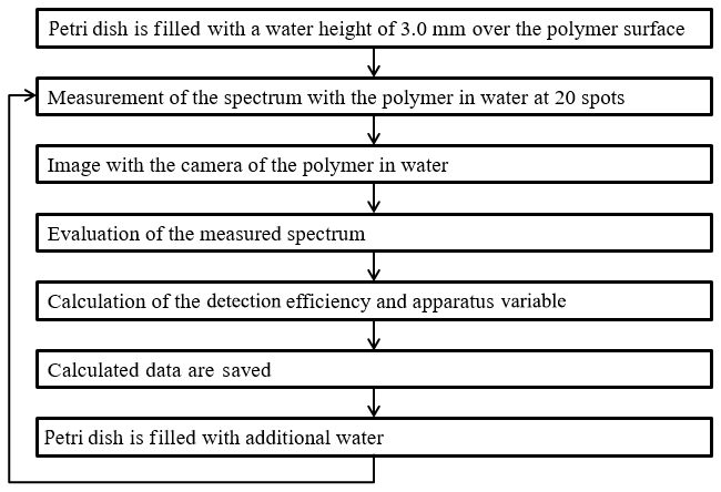
Figure 2 Flowchart for the measurement procedure of the polymer foils in 3.0, 4.5, 6.0, 7.0 and 8.0 mm water depth.

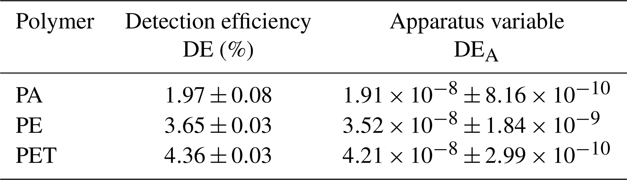
The measurements in dry conditions are done following the procedure described above in Sect. 2. The results are shown in Table 1 for the detection efficiencies and specific apparatus variables. The polymers are identifiable by their detection efficiency or their apparatus variable in dry conditions.

After determining the detection efficiency in dry conditions, the petri dish is filled to a water level of 3.0 mm water height over the plastic surface. After the 20 spots are measured, the spectra are saved into a table. The mini spectrometer has been replaced by the CMOS camera to take a picture of the polymer edge. The saved table is imported to MATLAB, and the mean values and the standard deviations are calculated assuming a Gaussian normal distribution. After the experiments with a water height of 3.0 mm, the petri dish is filled up to 4.5, 6.0, 7.0 and 8.0 mm with water. The procedure is repeated for every water level and every polymer.

Table 1 Experimental determined values for the detection efficiency and apparatus variable of the polymers PA, PE and PET.

3.4 Sample preparation

The examined polymer foils PA, PE and PET are cut into pieces of 2×2 cm and fastened in a petri dish using adhesive strips (see Fig. 3). This prevents the plastics from floating upwards, as they all have a lower density than water. The adhesive strips also have a fluorescence signal. Thus, only the parts of the polymers are illuminated which are not covered by the strips.

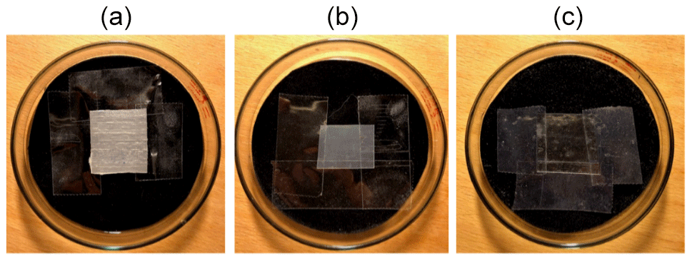
Figure 3 Polymer samples PA (a), PE (b) and PET (c) in a petri dish, attached with adhesive tape.

4 Experimental results with Setup 1 to identify the polymers in water

The evaluation of the measured data with Setup 1 shows that the apparatus variable and the detection efficiency change with an increasing water height. Figure 4 shows a decreasing detection efficiency (panel a) and the apparatus variable (panel b) as a function of the water layer.

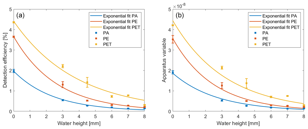
Figure 4 Representation of the fitting curves for the decreasing detection efficiency (a) and apparatus variable (b).

In order to determine the exponential decrease for both values, curves are fitted through the measured points of the detection efficiency and apparatus variable (see Fig. 4). The curves are modeled with an exponential fit following Eq. (5):

$$\begin{array}{}\text{(5)}& \mathrm{DE}=a\cdot \exp \left(b\cdot d_{\mathrm{W}}\right).\end{array}$$

The obtained values for the parameters a and b are entered in Table 2 for the fitted graphs of the detection efficiency and the apparatus variable, whereby the coefficient a indicates a polymer-specific value and b the intensity loss caused by the water in the setup. The values of coefficient b are identical, as they represent the optical losses due to the water in the setup. The values of coefficient a show no significant change if compared with the detection efficiency and apparatus variable in Table 1 because they are the polymer-specific values, which are measured in dry conditions. The goodness-of-fit parameter R² is calculated by the curve-fitting toolbox of MATLAB to determine how well the fitted graph fits the measured values (see Table 2). A value of R² close to 1 indicates that the curve fits the measured values almost exactly. The goodness-of-fit test shows that the fitted graphs represent the measured values with a very high probability.

Table 2 Determined coefficients a, b and R² of the exponential fit for detection efficiency DE and apparatus constant DE_A.

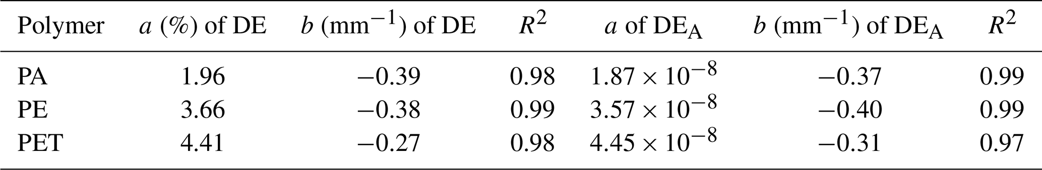
The coefficient b must not be interpreted as an absorption coefficient here because the absorption coefficient of water is 3 orders of magnitude smaller in the 400 nm wavelength region. The coefficient b includes all optical losses due to the water in the optical system of the microscope. The water layer acts like a lens here, and the focal plane of the objective lens of microscope is lost from which the detected light is emitted. Nevertheless, a fast and easy identification in tap water is possible with this technique.

5 Experimental results with Setup 2 to detect polymers in water

The pictures of the three polymer samples have been taken using Setup 2 with an exposure time of 0.1 s and a magnification of ×10 in water depths of 3.0, 6.0 and 8.0 mm. Figure 5 shows the pictures of PA (first row), PE (second row) and PET (third row), whereby the first one was taken in dry conditions, the second at 3.0 mm, the third at 6.0 mm and the fourth at 8.0 mm (from left to right). The measurements were done in different positions because the petri dish was removed from the microscope after each measurement in order to be filled to the next water level. After filling, the petri dish was placed under the microscope again, which leads to a new measuring spot. If the reemitted fluorescent light is low, a black artifact could be seen, which is caused by a third-party non-extractable particle in the microscope.

Figure 5 Images of the polymers PA, PE and PET in dry conditions and at 3.0, 6.0 and 8.0 mm water depths.

As the images show, a decrease of the fluorescence intensity is caused by the increasing water layer, but the polymers can be detected very well. PET has the highest fluorescence intensity, followed by PE and PA as the third row in Fig. 5 shows. The reason for this order is that PET has the highest detection efficiency, PE the second highest and PA the lowest; i.e., PET reemits more photons back to the camera than PE and PA. Thus, the detected fluorescence intensity of the camera is higher. In general, the detection of the polymers in water with the camera shows better results than the identification of the polymers in water with Setup 1. There is less effort to take one picture of a polymer sample in water than taking 20 measurements at different spots.

In order to also identify the polymers with a CMOS camera, the camera has to be calibrated with a probe normal. The fluorescence intensity could be measured in absolute dimensions and not only as a relative value. If absolute values were measured, an average value and a standard deviation could be calculated of all pixels of the image to determine the detection efficiency.

6 Conclusions

In summary, the experimental investigations have shown that plastics can be detected and identified in water. The previously published method has been extended with an optical loss coefficient for water in such a way that it is possible to detect and characterize the polymer samples in different water layers. The evaluation of experimental data shows consistent results with the detection efficiencies obtained earlier in Wohlschläger et al. (2019). An exponential decrease of the detection efficiency is observed as a function of the water layer thickness in the microscope setup. Although the optical effect of the water in the setup has a large influence, the identification of the plastics is still possible because the coefficient a of the detection efficiency and the apparatus variable are independent of the medium.

Unfortunately, the identification of real plastic samples in water is limited with this method because parameters like the thickness of the polymers are generally unknown but are required by the proposed model for identifying polymers with a detection efficiency and the apparatus variable.

The experiments have been successful in detecting the polymers in water due to their fluorescence behavior with an imaging system. For this purpose, the mini spectrometer has been replaced by a CMOS camera and an optical filter. Images have been taken with an exposure time of 0.1 s and a magnification of ×10 for each polymer. The results show that the polymers can be detected with an imaging system in water layers up to 8.0 mm. In general, it has been easier to detect the polymer films in water with the imaging system. Considering the non-optimized optical setup, it is expected that the detection and identification of microplastics in water can be further improved.

In the future, more experiments with both systems should be done. The influence of the water has to be further examined with different objectives. The exposure time of the camera could be increased to show if detection of the polymers is also possible in deeper water layers. Future investigations should also show whether the detection method can also be used to detect microplastics in water. If microplastics can be detected, further studies should prove that the microplastic particles can be distinguished from impurities like organic components, which are present in a high variety in real water samples. Also, other methods like fluorescence lifetime measurements may be applied to measure relative rather than absolute relationships of the fluorescence behavior of polymers.