the Creative Commons Attribution 4.0 License.
the Creative Commons Attribution 4.0 License.
 | 10 Nov 2020
Traceable measurements of harmonic (2 to 150) kHz emissions in smart grids: uncertainty calculation
Deepak Amaripadath
Etienne Toutain
Robin Roche
Fei Gao
The necessity of measuring harmonic emissions between 2 and 150 kHz is outlined by several standard committees and electrical utilities. This paper presents a measurement system and its traceable characterization designed to acquire and analyse voltages up to 230 V and currents up to 100 A with harmonics up to 150 kHz that may occur in smart grids. The uncertainty estimation is carried out and described in detail for both the fundamental and supraharmonics components. From a metrological point of view, ensuring the traceability of current measurements for frequencies higher than 100 kHz and dealing with the complexity of uncertainty determination are bottlenecks related to supraharmonics measurements that this paper proposes an approach to deal with.
- Article
(303 KB) - Full-text XML
- BibTeX
- EndNote


Although smart grid technology is deployed and operational in several countries, some areas of concern, such as power quality issues, still need technical improvements. The grid equipment is designed to satisfy the harmonic emission limits, but with an increased share of renewables and DC loads, the energy transfer is mediated by power electronics, which is a primary cause of high-frequency phenomena. Disturbances from these renewable energy sources are generally larger in magnitude, less regular and with a higher frequency than those from traditional generation sources and loads, making power quality (PQ) measurements difficult to perform. The state-of-the-art analysis indicates that supraharmonic emissions (emissions from grid equipment in the frequency range of 2 to 150 kHz) are a significant PQ issue in the smart grids (Klatt et al., 2013; Rönnberg et al., 2016). There is equipment, such as electrical appliances, photovoltaic inverters and electric vehicle chargers, that has power electronic converters with active and passive switching considered non-intentional sources of supraharmonic emissions, whereas transmitters of power line communication (PLC) are considered intentional sources of supraharmonic emissions. The effects of supraharmonic emissions, like interferences in the electrical network generating irregularities in the equipment operation (Unger et al., 2005; Zavoda et al., 2015) or interferences with PLC transmissions operating in the frequency range of 9 to 500 kHz (Rönnberg et al., 2011), can have a significant economic impact. It is therefore important to quantify supraharmonic emissions in order to detect and limit their harmful effects.
Recommendations concerning the measurement system and method exist in some standards (IEC, 2003, 2015). However, the suprahamonic emissions are mainly measured in a laboratory testing environment and for individual equipment. The artificial main networks are usually used to simulate the mains during these measurements, but their characteristics are representative of former electricity networks. Aiming at obtaining a representation of supraharmonic emissions occurring in a residential smart grid, we adopted an approach based on a metrologically characterized measurement system and the design of experiments (Montgomery, 2008). This innovative approach creates a multi-factor design to maximize the obtained information with a minimum number of measurements but relevant configurations. Both the method and the measurement system were used on Concept Grid, a French platform designed to study the new smart grid equipment. Details about the design of experiments and the measurement results are given in the PhD thesis (Amaripadath, 2019). The present paper focuses on the measurement system and its metrological characterization providing more details with respect to Istrate et al. (2020).
There are several papers (Rönnberg et al., 2017) that describe the measurement methods but very few (Klatt et al., 2013) dedicated to the measurement system or to the uncertainty calculation. The main challenges in measuring supraharmonic emissions between 2 and 150 kHz are (a) the low amplitudes of voltages and currents at high frequencies (from 1 % to less than 0.1 % of the 50 Hz voltage or current fundamental component) requiring high sensitivity and wide-band transducers to accurately detect these emissions and (b) the signal recording with high resolution and wide dynamic range to detect even the smallest emissions. The measurement system presented in this paper was designed to satisfy certain criteria listed below.
-
To use the dynamics and the resolution of the digitizer for the most accurate measurement. Voltage and current are acquired on four distinctive channels, the supraharmonic components being acquired once the 50 Hz components are filtered.
-
To ensure the electrical safety of the measuring devices and the operator by using an isolation transformer, an optical isolator and current sensors based on electromagnetic induction.
-
To have, as much as possible, sensors that connect to the power grid in a non-invasive way.
2.1 Setup constitution
The setup schematic is illustrated in Fig. 1, where EUT symbolizes the equipment under test connected to the grid (EV chargers, heat pumps, PV inverters, household appliances, etc.). The voltage is acquired on two channels: analog inputs AI0 and AI1. The isolating transformer with a ratio of 230 V : 10 V steps down the grid voltage, while the 2 : 1 resistive divider acts like a load for the transformer and reduces the voltage level to be compatible with the data acquisition card input. Signal processing of AI0-acquired data provides information about the 50 Hz fundamental voltage.
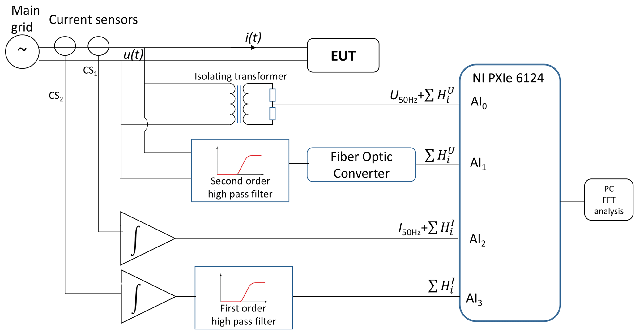
The supraharmonic voltage components are measured using channel AI1, which consists of a second order passive high-pass filter (HPF) with a cut-off frequency of 590 Hz that filters the fundamental component. The HPF is followed by an electrical-to-optic and optic-to-electrical converter system, which transmits analog and digital information via fiber optic cable. The isolation between the network and the recorder is ensured as well as the safety of both user and equipment.
The current is also acquired on two channels: AI2 and AI3. Two openable Rogowski coils are used as current sensors with the following characteristics:
-
current sensor CS1: 120 A peak current; 50 mV A−1 sensitivity; 0.23 Hz–0.6 MHz bandwidth;
-
current sensor CS2: 50 A peak current; 100 mV A−1 sensitivity; 0.45 Hz– 1.0 MHz bandwidth.
The 50 Hz current component is given by the analysis of AI2 data. To get the information on the (2 to 150) kHz current harmonics, a first-order high-pass filter (with 590 Hz cut-off frequency) is added before acquiring the data on AI3. The output voltages of the current sensors are compatible with the data acquisition input levels.
The data acquired from the electric grid with a 1 MS s−1 sampling rate are treated by software developed in LabView. The voltage and current waveforms in the time domain are converted into the frequency domain using the fast Fourier transform algorithm. The processing is performed on windows of 200 ms duration according to IEC (2003) and uses a flat-top window. The entire measurement setup was characterized and metrologically calibrated as described in the next section.
2.2 Traceable calibration and uncertainty
In order to identify the quality and the correction factors of the designed measurement system as well as to ensure its traceability, the constitutive components were calibrated at LNE, the French National Metrology Laboratory. The input voltages and currents used for characterization are selected based on the literature and real grid measurement analysis. The measured quantities are traceable to the International System of Units through the calibration of the reference voltage source, the standard current monitors, and the time base, all in reference to the national French primary standards.
All calibrations were performed in a controlled environment: temperature-regulated room at (23.0±1.0) ∘C, relative humidity of less than 60 %. The uncertainties generated by the temperature variations are negligible (10−6 order) compared with all other components. Therefore, they do not appear in the uncertainty budgets.
2.2.1 Acquisition of raw voltage on AI0
The raw voltage signal contains both the fundamental and harmonics components. It can be written as in Eq. (1):
where U1, f1 and ϕ1 denote the amplitude, the frequency and the phase of the fundamental component; Un and ϕn refer to the amplitude and the phase of the nth-order harmonic.
Even if the raw voltage is acquired on the AI0 channel, the researched information concerns mainly the fundamental component. Therefore, the whole acquisition channel was characterized for 50 Hz voltages up to 230 V. A high-accuracy voltage source (calibrator) was used to generate the necessary input voltage Ucal that varied from 100 to 230 V. The isolating transformer plus divider and the acquisition card with AI0 input (Fig. 1) were characterized simultaneously. The amplitude of the fundamental can be written as
where Ucal is the input voltage, represents the conversion coefficient to be applied for the whole acquisition chain and εdd, , εnoise, and εimped are the relative errors for daily drift, fast Fourier transform (FFT) windowing, signal noise and cable impedance.
The standard deviation of the conversion coefficient relative to its average value is and indicates a good linearity between 100 and 230 V. The average value is applied in computations, and the standard deviation is considered uncertainty.
By applying the law of propagation of uncertainties to Eq. (2) according to the guide to the expression of uncertainty (JCGM, 2008), the following relative combined uncertainty is obtained:
The combined uncertainty associated with U1 is composed of the standard uncertainties related to the following.
-
The voltage source, Ucal: the calibration, the drift between the emission of the calibration certificate and its use, the temperature fluctuation; the uncertainty is obtained from the calibration certificate.
-
The conversion coefficient, ; the uncertainties are given by the standard deviation of the linearity with the input voltage and the standard deviation of 20 repetitions.
-
The daily drift, εdd of the acquisition chain (in case of long-term voltage surveillance); the drift is followed over 1 week and is given by the slope of the linear fit of the measured voltage value: .
-
The FFT windowing, ; the amplitude of the 50 Hz fundamental was determined by applying a known input voltage and different FFT windows like Hanning, Hamming, Blackmann–Harris, Blackmann and flat top. The minimum relative error is obtained for a flat-top window. All further mathematical treatment includes this window. Since no correction is applied, the uncertainty term is the obtained relative error (JCGM, 2008).
-
The signal noise, εnoise; the effect of noise was estimated by injecting random noise from 0 % to 1 % of the fundamental amplitude. The maximum error obtained for 1 % added noise is considered uncertainty.
-
The cable impedance influence, εimped; the effect of impedance is studied by changing the length of the connection cables. The obtained error corresponds to 1 m coaxial cable length, 4 times greater than the reference.
Table 1Uncertainty budget for fundamental and (2 to 150) kHz voltage harmonics.

The contributions to the global uncertainty budget are listed in Table 1. The expanded uncertainty is obtained from the combined standard uncertainty by applying a coverage factor k=2 that corresponds to a coverage probability of 95.45 %.
2.2.2 Acquisition of (2 to 150) kHz voltage harmonics on AI1
The voltage supraharmonics are acquired on channel AI1 (Fig. 1) once the fundamental component is filtered. The transfer function of the measurement channel including the high-pass filter, the optical converter and the AI1 acquisition channel was obtained by varying the amplitude of the input voltage from 20 mV up to 3.5 V and its frequency from 2 kHz up to 150 kHz. This acquisition channel presents nonlinear variations with both the input voltage amplitude and the frequency. The gain variation of the transfer function presents higher nonlinearities for lower voltages (between 20 mV and 1.5 V). It is worth mentioning here that careful attention must be paid to the usage of a calibrator when voltages of less than 200 mV are generated. As it is designed for a 50 Ω load, it is necessary to use an inductive divider with gigaohm impedance as the load. Otherwise, the appropriate corrections must be applied. The high-pass filter of this acquisition channel has an impedance of 2 kΩ with influence on the characterization measurements. Therefore, corrections are applied for voltages from 20 mV to 1.5 V. The standard deviation of the gain values from 1.5 to 3.5 V is . The average value of the corrected gain is considered to determine the harmonic amplitudes, and the standard deviation is taken into account as the uncertainty component.
The frequency response reflects mainly the characteristic of the high-pass filter. Channel attenuation varies between 0.6 and 2 dB for frequencies between 2 and 10 kHz (higher attenuation for lower frequency). In this interval, the necessary corrections are applied. As previously, the average value of the corrected gain is used to determine the harmonic amplitudes, while the standard deviation, from 10 to 150 kHz, contributes to the uncertainty budget.
The uncertainty budget for the amplitude of voltage harmonics is obtained in a similar way to that for the 50 Hz voltage. Uncertainty components listed in Table 1 are estimated for 0.12 V and 20 kHz frequency.
2.2.3 Acquisition of raw current on AI2
The current signal is acquired by means of inductive sensors (Rogowski coil type) that generate a voltage proportional to the supply current. The equation that links the measurement results to the input current is
where and represent the amplitudes of voltages determined after acquisition for the fundamental component on channel AI2 and, for supraharmonics, on AI3; is the conversion coefficient of the Rogowski coil 1 and the AI2 channel and is the conversion coefficient of the Rogowski coil 2, the high-pass filter and the AI3 channel (Fig. 1).
Table 2Uncertainty budget for fundamental and (2 to 150) kHz current harmonics.
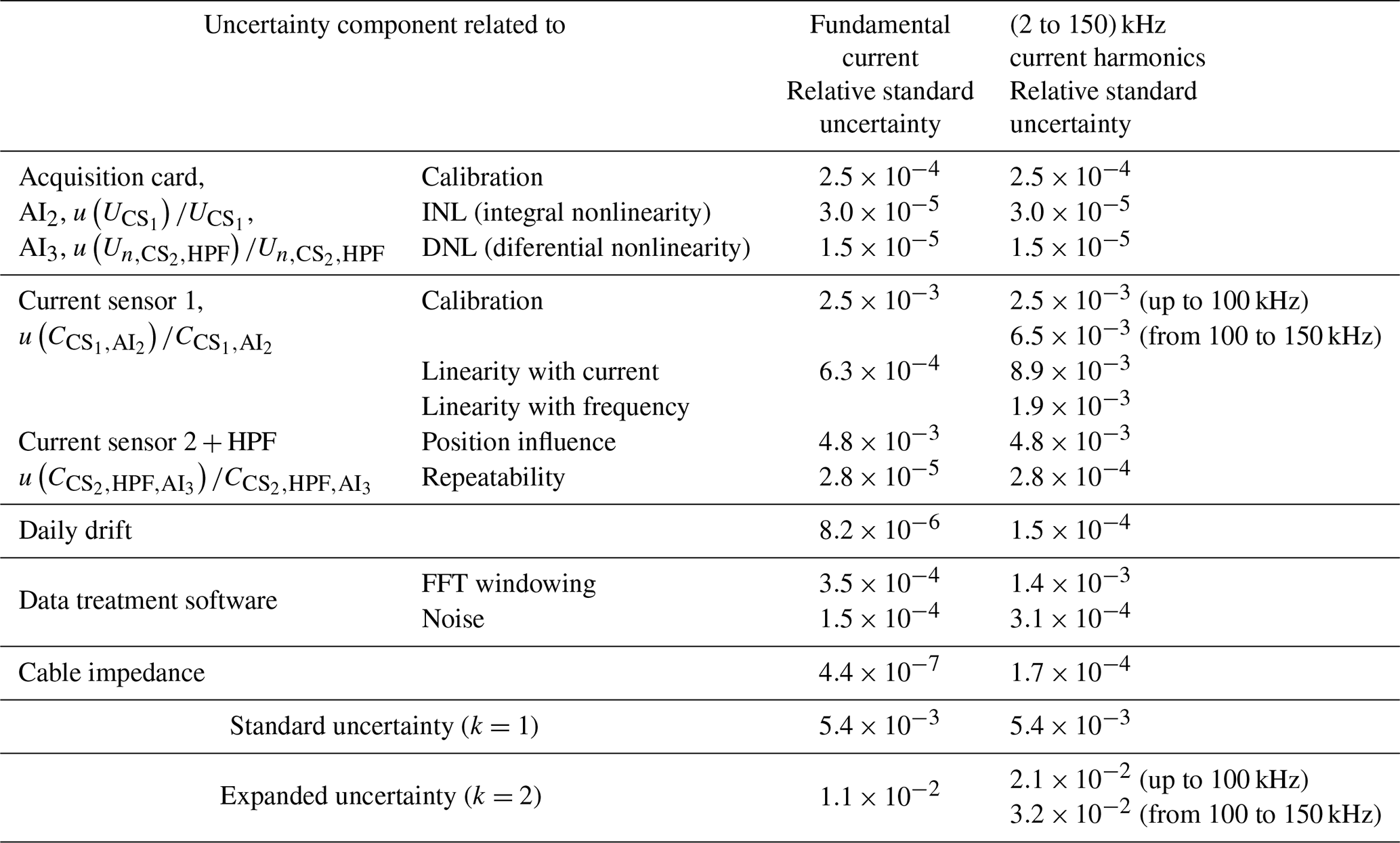
The AI2 acquisition channel is mainly used to determine the fundamental component of the current. The linearity of the conversion coefficient was verified for the interval 5 to 100 A with a 50 Hz sinusoidal current. The average value of the conversion coefficient, 48.6 mV A−1, is considered in the data treatment, and the relative standard deviation on the studied interval contributes to the uncertainty budget.
By applying the law of propagation of uncertainties to the first term of Eq. (4), the following relative combined uncertainty is obtained for the fundamental value of the current signal:
The uncertainty components determined by statistical methods (e.g., repeatability, noise), listed in Table 2, are estimated for the 100 A, 50 Hz sinusoidal current that generates 5.0 V.
2.2.4 Acquisition of (2 to 150) kHz current harmonics on AI3
Current-like voltage supraharmonics have low-level amplitudes (a few milliampères) for frequencies going up to 150 kHz. Considering the conversion coefficients of the current sensors, it is expected to measure very low voltages (10−6 to 10−3 V). Measuring such low voltages at 150 kHz requires careful attention (as mentioned in Sect. 2.2.2), but the traceability of these measurements can be ensured by national metrology institutes. It is more challenging to ensure the traceability of AC currents for frequencies higher than 100 kHz due to the rarity of the available methods (mainly AC/DC current transfer) and to the difficulties in generating hundreds of milliampères or more at frequencies higher than 100 kHz. The used current sensors are calibrated with the LNE-developed methods and standards (Fortune et al., 2014).
The transfer function of the measurement channel composed of the Rogowski coil 2, high-pass filter and AI3 acquisition channel is obtained for input currents with amplitudes varying from 20 mA to 1 A and frequencies from 2 to 150 kHz.
The gain variation with the current level presents a relative standard variation of with higher dispersion for lower currents (less than 200 mA). The average value of the conversion coefficient is used for further computations with the associated standard uncertainty.
The frequency response was obtained for 1 A input current of variable frequency. The obtained curve reflects the high-pass filter characteristic with a higher attenuation of frequencies between 2 and 5 kHz. The necessary corrections are applied. The standard deviation of the conversion coefficient relative to the average value is from 5 to 150 kHz.
All other uncertainty components are estimated for the 200 mA, 150 kHz input current signal. Table 2 presents the uncertainty budget for the amplitude of (2 to 150) kHz harmonics.
A measurement platform was designed to study the supraharmonic emissions in the grid in the frequency range of 2 to 150 kHz. Its metrological characterization is described in detail. The obtained expanded uncertainties with a coverage factor of k=2 (95.45 % coverage probability) are for the 50 Hz voltage, for (2 to 150) kHz voltage harmonics, for the 50 Hz current, and for the (2 to 150) kHz current harmonics. The obtained uncertainties for the (2 to 150) kHz harmonics are less than ±5 % for the measured values as requested by the IEC (2003) standard. The highest uncertainty, 3.2 %, is obtained for the measurement of current harmonics for frequencies higher than 100 kHz. The current sensor and the high-pass filter introduce the most important uncertainty components. The higher uncertainties for supraharmonics are due to the low level of voltages and currents (10−3 order). Therefore, the obtained uncertainties can be reduced through improvements in the linearity of filters and current sensors and through the implementation of digital signal processing algorithms.
The values presented in the article are based on the following:
-
the CMCs (Calibration and Measurement Capabilities) of LNE declared on KCDB (https://www.bipm.org/kcdb/, last access: 9 November 2020) (KCDB, 2020);
-
the calibration certificates existing in the LNE laboratory (these contribute to guarantee the measurement traceability to the International System of Units);
-
the results of characterizations presented in detail in the thesis Amaripadath (2019).
DI, DA and RR contributed to conceptualization, investigation, validation and writing. DI, DA and ET performed data curation and acquisition, investigation, and formal analysis. DI and DA proposed the methodology. DI, RR and FG ensured the project administration and supervision.
The authors declare that they have no conflict of interest.
This article is part of the special issue “Sensors and Measurement Science International SMSI 2020”. It is a result of the Sensor and Measurement Science International, Nuremberg, Germany, 22–25 June 2020.
The main work was performed under the H2020 MEAN4SG project (grant number 676042 MEAN4SG). The validation work and the open-access publication fees are covered by the 18NRM05 SupraEMI project.
This paper was edited by Klaus-Dieter Sommer and reviewed by two anonymous referees.
Amaripadath, D.: Development of Tools for Accurate Study of Supraharmonic Emissions in Smart Grids, PhD thesis, Université Bourgogne Franche-Comté, France, 199 pp., available at: https://tel.archives-ouvertes.fr/tel-02498270 (last access: 9 November 2020), 2019.
Fortune, D., Istrate, D., Ziade, F., and Blanc, I.: Measurement method of AC current up to 1 MHz, in: Proc. of 20th IMEKO TC-4, 15–17 September 2014, Benevento, Italy, 35–39, 2014.
IEC: EMC Part 4–7: Testing and measurement techniques – General guide on harmonics and interharmonics measurements and instrumentation, for power supply systems and equipment connected thereto, IEC 61000-4-7, 2003.
IEC: EMC Part 4–30: Testing and measurement techniques – Power quality measurement methods, IEC 61000-4-30, 2015.
Istrate, D., Amaripadath, D., Toutain, E., Roche, R., and Gao, F.: Traceable Measurements of Harmonic (2−) Emissions in smart Grids, in: Proc. of SMSI, 22–25 June 2020, Nuremberg, Germany, https://doi.org/10.5162/SMSI2020/E3.2, 2020.
JCGM: 100: 2008: Guide to the expression of uncertainty in measurement (GUM), BIPM, available at: https://www.bipm.org/fr/publications/guides/gum.html (last access: 9 November 2020), 2008.
KCDB: Calibration and Measurement Capabilities – CMCs, available at: https://www.bipm.org/kcdb/, last access: 9 November 2020.
Klatt, M., Meyer, J., Schegner, P., Koch, A., Myrzik, J., Darda, T., and Eberl, G.: Emission Levels Above 2 kHz – Laboratory Results and Survey Measurements in Public Low Voltage Grids, CIRED, IET, 10–13 June 2013, Stockholm, Sweden, 1–4, https://doi.org/10.1049/cp.2013.1102, 2013.
Montgomery, D. C.: Design and Analysis of Experiments, 7th Edn., John Wiley & Sons, New York, USA, 2008.
Rönnberg, S. K. and Bollen, M. H. J.: Power Quality Issues in the Electric Power System of the Future, Elect. J., 29, 49–61, https://doi.org/10.1016/j.tej.2016.11.006, 2016.
Rönnberg, S. K., Bollen, M. H. J., and Wahlberg, M.: Interaction between Narrowband Power-Line Communication and End-User Equipment, IEEE T. Power Deliv., 26, 2034–2039, 2011.
Rönnberg, S. K., Bollen, M. H. J., Amaris, H., Chang, G. W., Gu, I. Y. H., Kocewiak, L. H., Meyer, J., Olofsson, M., Ribeiro, P. F., and Desmet, J.: On waveform distortion in the frequency range of 2 kHz–150 kHz – Review and research challenges, Elect. Power Syst. Res., 150, 1–10, 2017.
Unger, C., Krüger, K., Sonnenschein, M., and Zurowski, R.: Disturbances due to Voltage Distortion in the kHz Range – Experiences and Mitigation Measures, in: 18th International Conference and Exhibition on Electricity Distribution (CIRED), Turin, Italy, 1–4, 2005.
Zavoda, F., Ronnberg, S. K., Bollen, M. H. J., Meyer, J., and Desmet, J.: Power Quality and EMC Issues with Future Electricity Networks, in: Proc. of 23rd CIRED, 15–18 June 2015, Lyon, France, 1–5, 2015.