the Creative Commons Attribution 4.0 License.
the Creative Commons Attribution 4.0 License.
 | 27 Nov 2020
Random gas mixtures for efficient gas sensor calibration
Tobias Baur
Manuel Bastuck
Caroline Schultealbert
Tilman Sauerwald
Andreas Schütze
Applications like air quality, fire detection and detection of explosives require selective and quantitative measurements in an ever-changing background of interfering gases. One main issue hindering the successful implementation of gas sensors in real-world applications is the lack of appropriate calibration procedures for advanced gas sensor systems. This article presents a calibration scheme for gas sensors based on statistically distributed gas profiles with unique randomized gas mixtures. This enables a more realistic gas sensor calibration including masking effects and other gas interactions which are not considered in classical sequential calibration. The calibration scheme is tested with two different metal oxide semiconductor sensors in temperature-cycled operation using indoor air quality as an example use case. The results are compared to a classical calibration strategy with sequentially increasing gas concentrations. While a model trained with data from the sequential calibration performs poorly on the more realistic mixtures, our randomized calibration achieves significantly better results for the prediction of both sequential and randomized measurements for, for example, acetone, benzene and hydrogen. Its statistical nature makes it robust against overfitting and well suited for machine learning algorithms. Our novel method is a promising approach for the successful transfer of gas sensor systems from the laboratory into the field. Due to the generic approach using concentration distributions the resulting performance tests are versatile for various applications.
- Article
(5024 KB) - Full-text XML
- BibTeX
- EndNote


Despite impressive advances in sensitivity, selectivity and response time of gas sensor systems over the last decades (Marco and Gutierrez-Galvez, 2012; Sharma et al., 2018), there is a striking lack of publications on successful field tests or real-world applications. A search on Google Scholar (from 31 March 2020) returns more than 3.4 million results for “gas sensor + material” and 553 000 results for “gas sensor + “data processing””, but only around 28 000 results for “gas sensor + “field test””. At the same time, field tests are a crucial link to the successful implementation of gas sensors in large-volume consumer applications (Borrego et al., 2016; Castell et al., 2017). Also, from our own experience field test data very often are hard to interpret due to deviations from the ideal conditions during the original lab calibration, for example in terms of baseline and dynamics. We believe that one main issue hindering successful field tests is the lack of appropriate realistic calibration procedures for modern gas sensor systems. Calibration is only a side note in many works, as a vehicle to show the performance of a new material or data processing method. The experimental design often consists of a few fixed concentration levels per gas, and, in many cases, the sensor is exposed to one and only one target gas at a time. The resulting data are relatively easy to evaluate in terms of sensitivity, selectivity and speed of response, but of little use for complex real-world scenarios.
Virtually all applications – for example, air quality (Castell et al., 2017; Spinelle et al., 2017), fire detection (Kohl et al., 2001; Fonollosa et al., 2016), detection of explosives (Tomchenko et al., 2005; Yu et al., 2005) and breath analysis (Bajtarevic et al., 2009; Lourenço and Turner, 2014) – require selective, quantitative measurements in an ever-changing background of interfering gases. A sensor calibration with single substances (as, for example, in the datasets of Fonollosa et al., 2015a, b; Fonollosa, 2016; Bastuck and Fricke, 2018) does not reveal any masking effects or other gas interactions altering the sensor response. Some publications take this into account by performing calibration with gas mixtures (Sundgren et al., 1991; Wolfrum et al., 2006; Zhang et al., 2013; Fonollosa, 2015; Sauerwald et al., 2018). Most of these except two (Zhang et al., 2013; Fonollosa, 2015) use between three and five fixed concentration levels for each gas. This quantization of a continuous quantity can, with too few levels, easily lead to overfitting due to systematic errors in the experimental equipment, contamination1 of validation data through repetitions or misleading model performance measures.
In the past we could show good results in interlaboratory tests, as a first step towards a transferable calibration, with sequential calibration (Spinelle et al., 2017; Bastuck et al., 2018a; Sauerwald et al., 2018). However, there is still a gap between calibrating a sensor for interlaboratory tests and real-word scenarios (Sauerwald et al., 2018; Karagulian et al., 2019).
In this paper, we present and test a calibration scheme based on the method of random effects (Oehlert, 2000). It tackles the mentioned issues by drawing random concentrations from predefined distributions of a, theoretically, arbitrary number of gases. The result is a large number of gas exposures for calibration, each a unique mixture of all available gases. The approach is easy to configure and use, can be applied to a wide range of target applications, and is shown to be superior to sequential calibration.
2.1 Study design
The calibration method with randomized gas mixtures is shown using the example of indoor air quality (IAQ) but can be applied to any application and target variable. The gases used for this study were chosen to represent different approaches in IAQ assessment. Volatile organic compounds (VOCs) are an important indicator of IAQ, as many of the substances show irritating or even toxic behavior. Generally, a VOC is any organic compound that can be found in the gas phase at room temperature. The European Union defines VOC as any organic compound with an initial boiling point less than or equal to 250 ∘C measured at standard pressure of 101.3 kPa (Anon, 2004). In analytical chemistry these VOCs are normally divided into three subgroups: very volatile organic compounds, volatile organic compounds and semi-volatile organic compounds. Specific sampling and measurement protocols are associated with each group. However, from a health perspective, there is no need to treat these groups separately since both toxic and harmless compounds can be found in each. We will, therefore, subsume all three groups under the term VOC for direct-measuring gas sensor systems. The total sum of VOCs, TVOC (total VOCs), is one target value that can be used for calibration and is, for example, defined by the German Environment Agency (UBA) for IAQ classification (Seifert, 1999; Anon, 2007). A study on behalf of the UBA (Hofmann and Plieninger, 2008) lists the statistical distribution of more than 300 different VOCs in indoor environments. The VOCs can be divided into interfering VOCs and target VOCs with regard to human health: while the former are harmless in usual concentrations, the latter are mostly toxic or carcinogenic. Measuring all of these hundreds of VOCs in varying concentrations is not feasible, so a preselection must be made based on the expected concentrations. Since our equipment (Helwig et al., 2014; Leidinger et al., 2018) is limited to six gases plus humidity, two representatives each were selected for inorganic background gases, interfering VOCs and target VOCs.
The carrier gas stream consists of zero air with varying humidity plus the background gases carbon monoxide and hydrogen. Carbon monoxide is a ubiquitous gas with highly variable concentrations ranging from the atmospheric background at 150 ppb (Schleyer et al., 2013) up to several ppm (WHO Regional Office for Europe, 2010). The atmospheric background concentration of hydrogen is 500 ppb (Schleyer et al., 2013). We could not find any studies on H2 concentration in indoor air. We assume large fluctuations up to the ppm range (Schultealbert et al., 2018b) since hydrogen is emitted by humans (Levitt, 1969; Tomlin et al., 1991) and can, like CO2, be another indicator for human presence. For interfering VOCs we selected acetone and toluene, two common representatives with high average concentrations (Hofmann and Plieninger, 2008) but negligible health effects. The interfering gases were added to achieve a realistic TVOC concentration in indoor air (Hofmann and Plieninger, 2008). To represent the TVOC concentration with only two gases, they are supplied at 10 to 20 times the typical indoor concentrations. The target VOCs are two carcinogenic gases, formaldehyde and benzene. The concentration range of these target gases is based on the observed statistical distribution in indoor air (Hofmann and Plieninger, 2008) and WHO guidelines (WHO Regional Office for Europe, 2010; Anon, 2016). Since only a limited number of VOCs are present in this configuration, the sum of all measured VOCs is defined as VOCsum to clearly distinguish it from the common TVOC term.
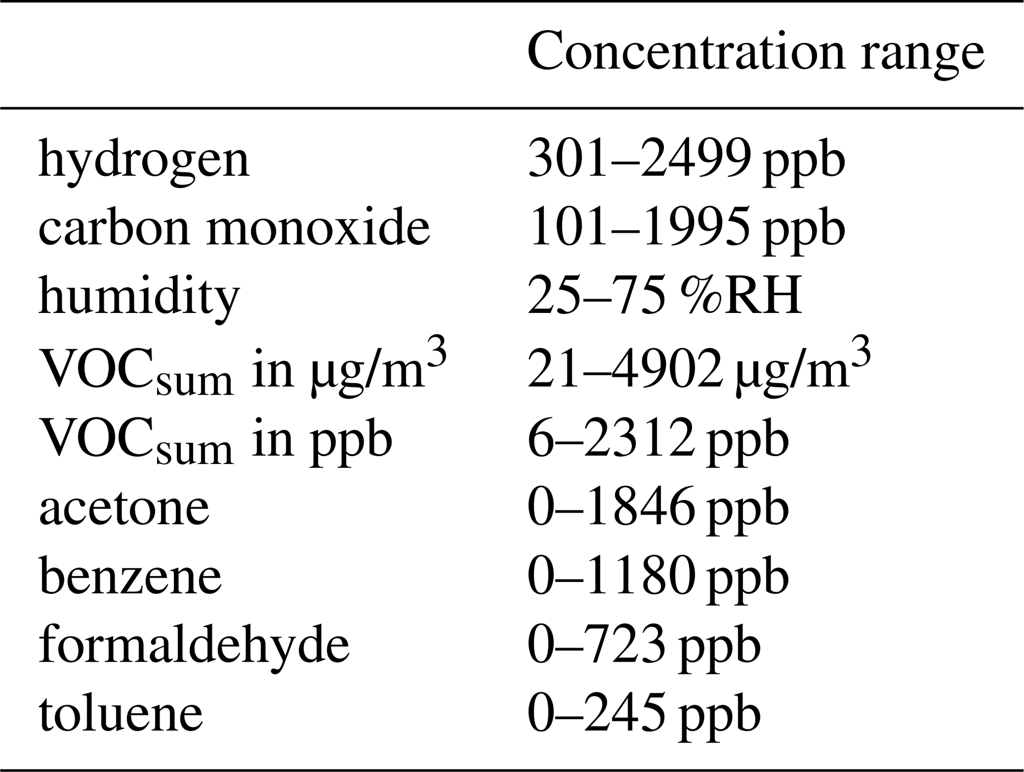
The random mixtures were generated using a Python script (Bastuck, 2019) which iteratively determines the ratios of all components as shown schematically in Fig. 1. To generate a randomized gas mixture, the concentrations of the background components (carbon monoxide, hydrogen and humidity) and VOCsum were varied independently of each other. The concentrations of humidity, carbon monoxide, hydrogen and VOCsum are uniformly distributed over a realistic range (see Table 1). For the generation of the single VOC concentrations, the randomly selected VOCsum concentration is divided into several steps. First, the ratio of interfering (VOCinterfering) and target (VOCtarget) VOCs in VOCsum is randomly selected to be between 0 and 20 % target VOC. Second, VOCinterfering and VOCtarget are again divided randomly into the individual VOCs, both with a ratio between 0 and 100 %. The parameters for the generation are shown in Table 1, and the resulting concentration ranges for the single gases and VOCsum in Table 2.
Due to an error in the measurement setup, the concentrations of toluene and benzene were swapped, and the concentrations planned for benzene were offered as toluene and vice versa. Therefore, the concentration levels of the carcinogenic benzene are rather high in this study compared to their true occurrence, while the concentrations of toluene are unusually low (ppb range). This does not have any impact on the general conclusions drawn from this experiment, but the results for selective quantification of these two VOCs should be interpreted with caution. The concentration distributions of the individual gases can be found in Fig. A1. Each randomized gas mixture was supplied to the sensors for 20 min each. Twelve measurements with 99 randomized gas mixtures each were conducted over a period of 5 weeks, resulting in a total of 1188 randomized gas mixtures.
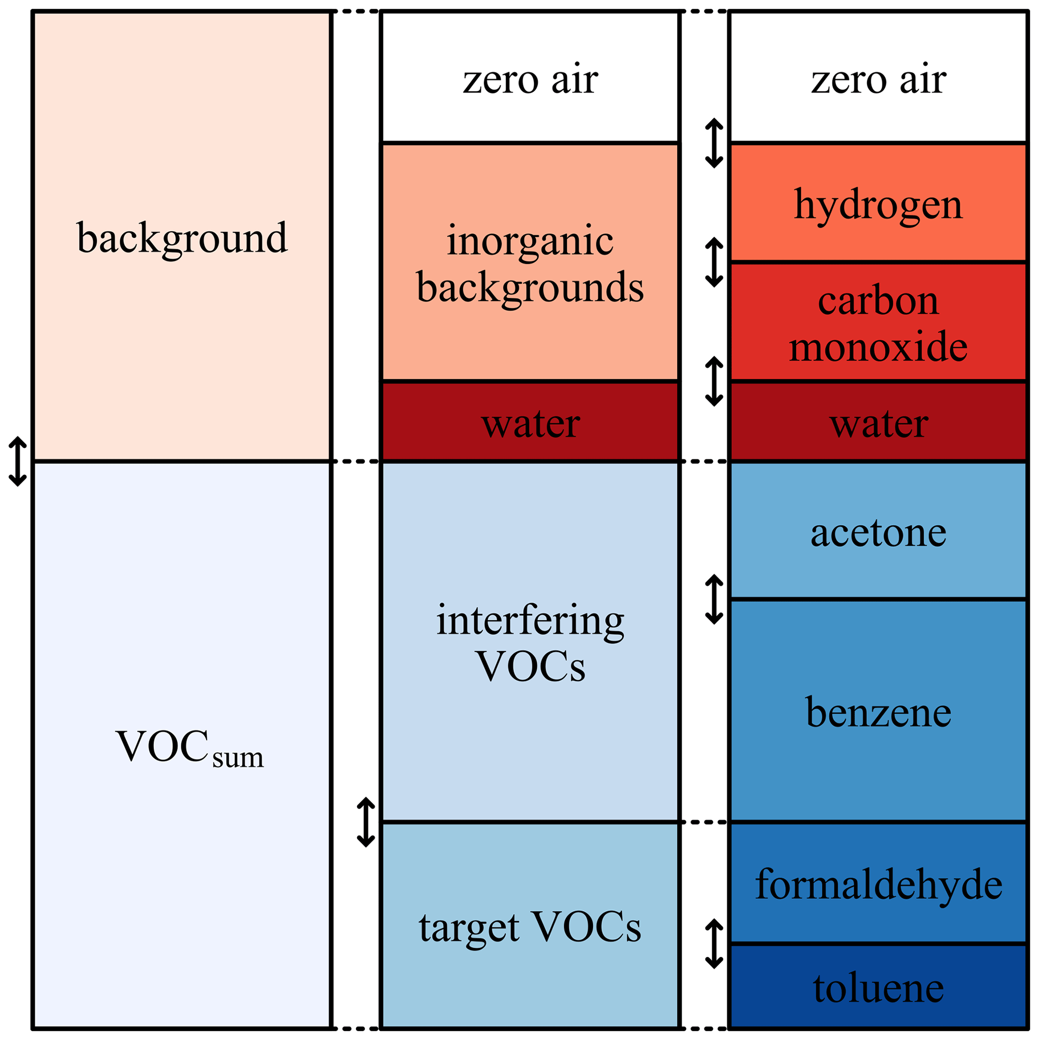
Figure 1Schematic overview of the random gas mixture generation. The scheme can be adapted to reflect different applications. Please note that this figure represents the measurement as it was actually performed, taking into account the accidental swapping of benzene (which should have been a target) and toluene (which should have been an interferent).
Table 1Parameters for the generation of randomized gas mixtures.
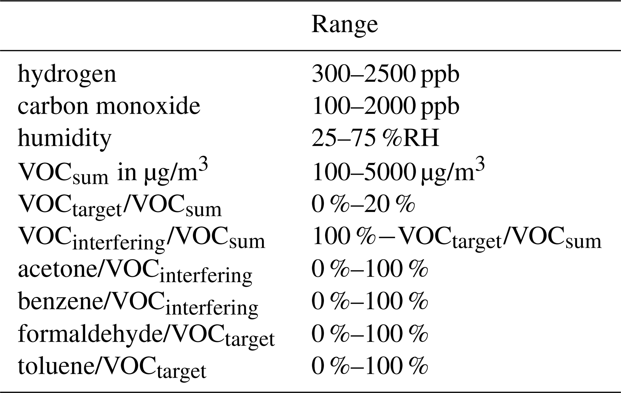
Table 2Resulting concentration ranges by the generation of randomized gas mixtures.
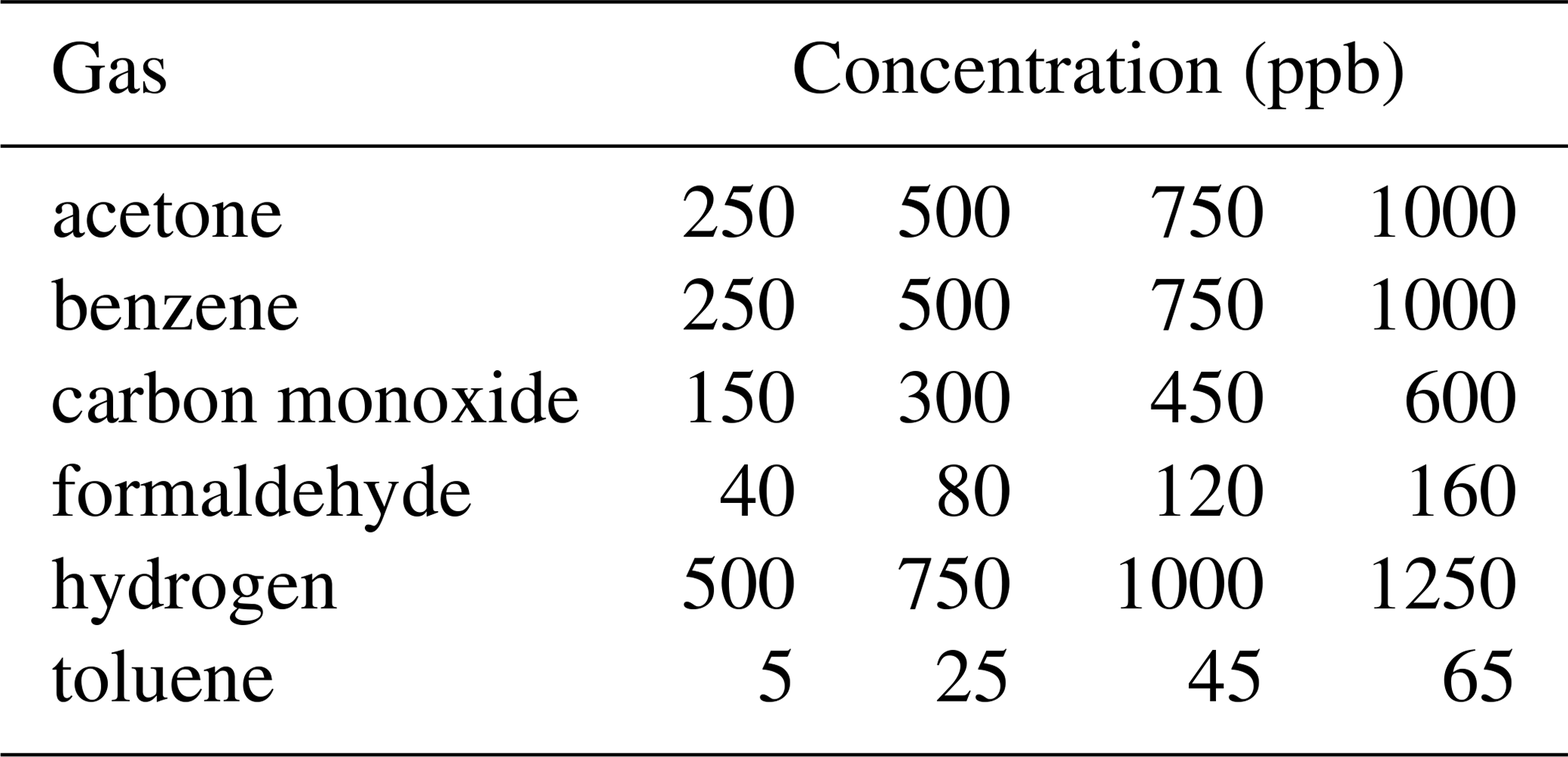
To compare the performance of our novel approach with a conventional sequential calibration strategy (one gas at a time, ascending concentration levels), a gas profile of this kind was measured for comparison. Each gas was supplied at four different concentrations (see Table 3), which were kept constant for 20 min. The background gases (hydrogen and carbon monoxide) were always kept at their atmospheric concentrations (500 and 150 ppb) except during their exposures as target gas. The profile was repeated three times at different relative humidities – 25, 50 and 75 %RH – resulting in a total of 72 different gas exposures. The comparison was made only for the gas concentration ranges which were common to both calibration profiles.
Table 3Gas concentrations used for the sequential calibration.
2.2 Setup
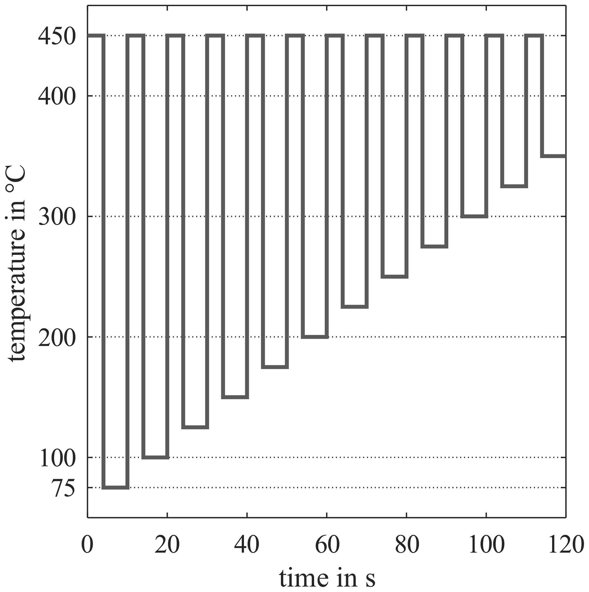
In the overall measurement setup, a total of 11 different sensors were tested, seven of them metal oxide semiconductor gas sensors (MOS) and four gas-sensitive field effect transistors (GasFET). An overview of the results of all systems for a reduced dataset with the last five measurements and a slightly different evaluation method can be found in Bastuck (2019). The results and findings in this paper are shown for two analog sensors from ams, namely AS-MLV and AS-MLV-P2.They were chosen due to our long experience with these two types of sensors (Baur et al., 2015, 2018b; Schütze et al., 2017; Schultealbert et al., 2018a). In recent interlaboratory tests we have also found that transferring a sensor calibration from one laboratory to another works with these types of sensor. However, we have also seen that missing gas concentrations can lead to misinterpretation in our models. In Sauerwald et al. (2018) we trained interfering gases with only a few gas concentrations, since each additional concentration would have meant a doubling of time. Therefore, we had problems with an extended humidity range, which was not covered by our calibration. In Bastuck et al. (2018a) we had a similar problem with hydrogen. Those previous issues make them good candidates for this study on a more efficient calibration strategy. The sensors were not operated in the operating modes recommended by the respective manufacturers, but with a self-designed temperature-cycled operation (TCO) (Gramm and Schütze, 2003; Baur et al., 2015; Schütze and Sauerwald, 2019). The temperature cycle is chosen to benefit from the highly sensitive differential surface reduction (DSR) method (Baur et al., 2018b). The total cycle for the presented sensors with a duration of 120 s is shown in Fig. 2. The MOS sensors were operated with electronics with logarithmic conductance measurement and resistance-based temperature control developed in our lab (Baur et al., 2018a).
The gas mixtures were supplied by our gas mixing apparatus (GMA), which is described in detail in Helwig et al. (2014) and Leidinger et al. (2018). It consists of several mass flow controllers (MFCs) to supply carrier gas (zero air) and add the desired gas concentrations from gas cylinders. A two-stage cleaning process generates the zero air (Leidinger et al., 2018). Hydrocarbons (larger than C3) are removed efficiently in the first step with a carbon filter system. In the second step, humidity is removed with a pressure swing, and smaller hydrocarbons as well as hydrogen and carbon monoxide are removed by catalytic conversion. The test gases from the cylinders are diluted twice to achieve very low and highly variable concentrations while avoiding the impact of different impurities contained in the synthetic air (Helwig et al., 2014). Humidity is supplied from a washing bottle with HPLC-grade water at room temperature (22 ∘C), which is flushed with zero air at the desired flow rate.
Since several sensors ran in the same experiment and should not affect each other, the total flow of 400 mL / min supplied by the GMA was split into four independent lines. To ensure proper split ratios, flow restrictions (10 cm of 1∕16”) were installed in each line, dominating the total flow resistance of each line, given that the rest of the setup is built with 1∕8” tubing (<25 cm per line, PTFE and stainless steel). The sensor chambers are made of PTFE and aluminum.
2.3 Evaluation methods
The evaluation is performed with the open-source software DAV3E (Bastuck et al., 2018b) and can be divided into five steps: feature extraction, dimensionality reduction, regression, hyperparameter optimization and testing. For feature extraction, the 120 s sensor cycle is divided into 120 equidistant ranges. In each of these ranges, the mean value and slope, in total 240 features per sensor cycle, are computed. To prevent overfitting during modelling, a dimensionality reduction with principal component analysis (PCA) is carried out. For the next steps of modelling, the first 20 principle components are used as features. The quantification of the desired target value (concentration of a single gas or a partial gas mixture, e.g., VOCsum) is performed with partial least squares regression (PLSR). For hyperparameter optimization and testing we use two different procedures. For evaluations with reduced datasets of the measurement we use the holdout method for testing; for instance, 10 % of the dataset is excluded from training. For hyperparameter optimization – i.e., the determination of the number of PLSR components – a 10-fold cross-validation is applied. For evaluations with the complete dataset, a nested cross-validation, also known as double cross-validation (Stone, 1974), is performed for testing and hyperparameter optimization. We perform an outer 10-fold cross-validation for testing, by randomly dividing the data in 10 parts once. One part in turn is set aside as the test dataset, while all other parts comprise the training dataset and are used to optimize the hyperparameters of the model. For this optimization, we also perform a 10-fold cross-validation on the training dataset for different numbers of PLSR components. In the inner loop, the training dataset of the outer loop is also randomly divided into 10 parts; nine parts are used for training and one for the hyperparameter validation. For nested cross-validation we treat all sensor cycles within the same gas exposure as one unit (group-based). Otherwise, very similar cycles could end up in both the training and test dataset of an iteration, effectively “contaminating” the training data and leading to over-optimistic performance estimates. The mean predictive performance for these validation sets is calculated for each number of PLSR components over the inner and outer loop. The best number of PLSR components is decided as the minimal number of PLSR components still giving a good2 predictive performance.
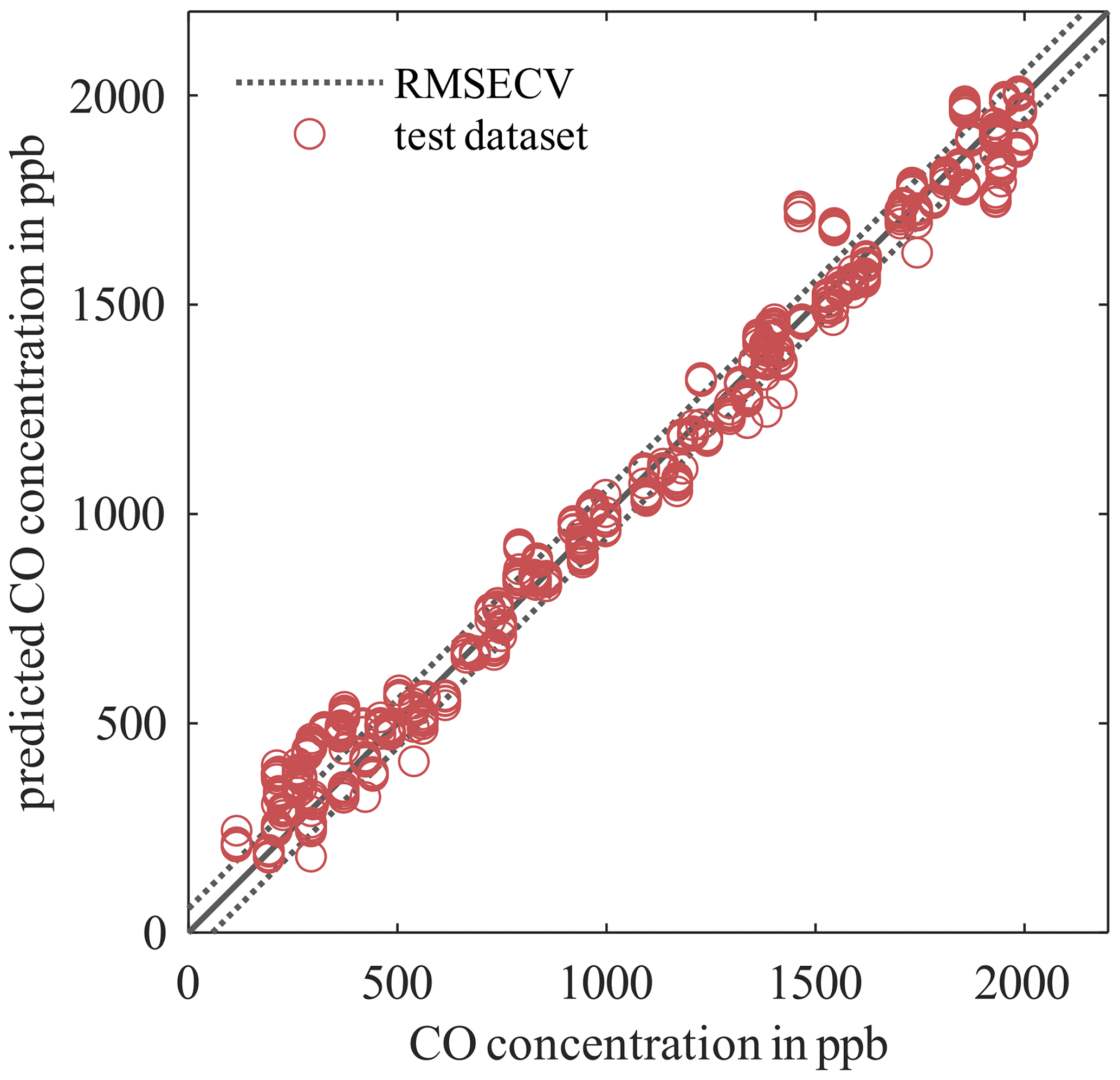
Figure 3PLSR model for the AS-MLV-P2 for quantification of carbon monoxide (CO). The model was calculated and 10-fold cross-validated from a reduced dataset with 198 randomized gas mixtures (measurements 8 and 9). The model was tested with 99 randomized gas exposures containing seven cycles each (measurement 10, open circles).
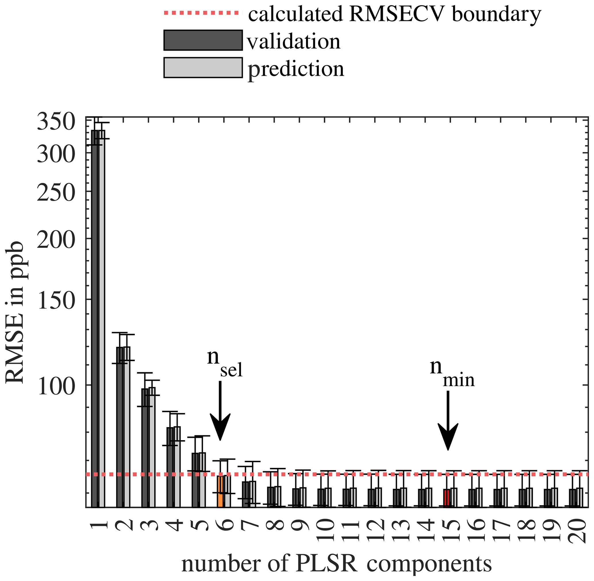
Figure 4Calculated RMSECV (hyperparameter optimization) and RMSEP (testing) with error bars depending on the number of PLSR components for the AS-MLV-P2 for the carbon monoxide model. The dotted red line indicates the boundary for the calculation of the minimum number of PLSR components, and the orange marked bar shows the RMSECV at the resulting number of components according to Eq. (2).

Figure 5Coefficient of determination (R2) for AS-MLV and AS-MLV-P2 for different models. Calculation of the regression model with the complete dataset with 10-fold nested cross-validation for hyperparameter optimization (PLSR components) and testing. The number of PLSR components of the model, determined with Eq. (2), is given in parentheses.
Generally, different metrics are used to describe the performance of a regression model. Arguably the most prevalent is the coefficient of determination R2, which describes the ratio of the explained to the total variance. Its range from 0 to 100 % is, however, hard to interpret in terms of, for example, accuracy and precision of a model. This interpretation becomes much easier for the root-mean-square error (RMSE) since it has the same unit as the model output. A distinction is made between the RMSE of calibration (RMSEC) for the training, the RMSE of cross-validation (RMSECV) for hyperparameter optimization and the RMSE of prediction (RMSEP) for testing. However, expecting the same precision between two models covering different concentration ranges is unrealistic. An RMSE of 50 ppb would be considered quite poor for formaldehyde (having an exposure limit of 80 ppb) but excellent for hydrogen. Since we choose the concentration ranges for all gases based on realistic data, it seems natural to define a metric “dynamic range” (DNR) as
with the maximum concentration cmax, t and the root-mean-square error RMSEt for the target t. While not transferrable to arbitrary applications, the DNR allows comparison of sensor and model performances for different gases and concentration ranges in this case.
To find the optimal number of PLSR components, we calculate the for each number of PLSR components n∈N, for all 10 cross-validation folds in all 10 testing folds . Thereby, the maximum number of PLSR components is limited to the number of predictor variables, in this case, the 20 first principle components. The RMSECVn is the mean value over all folds at the same n. We selected the number of PLSR components nsel with Eq. (2). This means we take the minimum number of PLSR components for which the RMSECVn is less than the plus the standard deviation of at the point of the minimum. A visualization of the data evaluation procedure can be found in Appendix B as pseudocode. Figure 4 shows the selection of the best number of PLSR components according to Eq. (2).

Figure 6Root-mean-square error of prediction (RMSEP) for AS-MLV and AS-MLV-P2 for different models. Calculation of the regression model with the complete dataset with 10-fold nested cross-validation for hyperparameter optimization (PLSR components) and testing. The number of PLSR components, determined with Eq. (2), is given in parentheses.
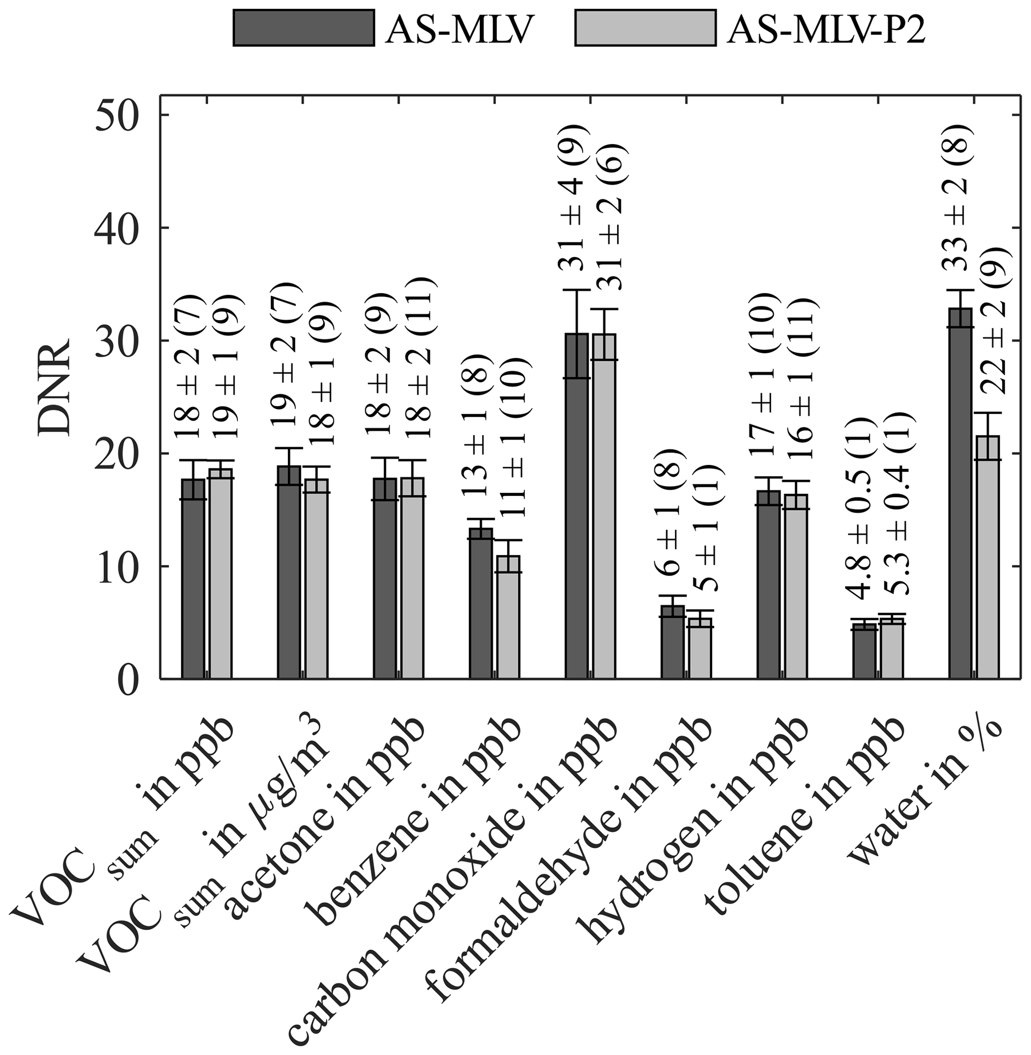
Figure 7Dynamic range (DNR) for AS-MLV and AS-MLV-P2 for different models. Calculation of the regression model with the complete dataset with 10-fold nested cross-validation for hyperparameter optimization (PLSR components) and testing. The number of PLSR components, determined with Eq. (2), is given in parentheses.
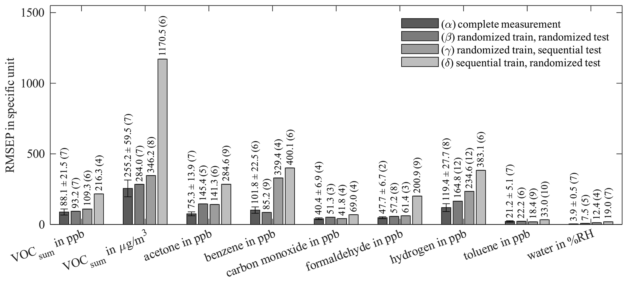
Figure 8Root-mean-square error of prediction (RMSEP) of AS-MLV-P2 for different training and testing models. All models use 10-fold cross-validation for hyperparameter optimization; the resulting number of PLSR components, determined with Eq. (2), is given in parentheses. A detailed description of (α)–(δ) is given in Table 4.
Twelve measurements were performed. Each of the 1188 gas exposures contains 10 sensor cycles. Due to the time constant of the gas exchange, we omitted two sensor cycles at the beginning and one cycle at the end of the gas exposure in the evaluation. Therefore, we have a total of seven useful cycles per gas exposure, amounting to 8316 from the complete measurement campaign. Two and a half measurements (numbers 5, 6 and 7), in sum 245 random gas exposures, had formaldehyde completely missing because the bottle had run empty. Additionally, 74 random gas exposures are missing for the AS-MLV-P2 and 115 for the AS-MLV due to issues with the sensor system. Therefore, we can use 828 (AS-MLV) or 869 (AS-MLV-P2) random gas exposures for formaldehyde models and 1073 (AS-MLV) or 1114 (AS-MLV-P2) for all other models.
Figure 3 shows an example of a PLSR model for the AS-MLV-P2 for quantification of carbon monoxide. For better visualization we reduced the dataset: this model was trained with 198 randomized gas exposures (measurements 8 and 9); the hyperparameter optimization was done by 10-fold cross-validation. The dotted lines show the RMSECV of the hyperparameter optimization; the red circles show the predicted carbon monoxide concentration from 99 additional randomized gas exposures (measurement 10). A good agreement of the reduced dataset with an RMSECV of 57.3 ppb and a RMSEP of 73.9 ppb is found. This means the unknown measurement can be predicted with a DNR of 27 in the range of 100 to 2000 ppb carbon monoxide.
For the evaluation of the complete measurement campaign, 10-fold nested cross-validation is used. Figure 4 shows the hyperparameter optimization for the selection of the number of PLSR components according to Eq. (2) as an example for the quantification of carbon monoxide with the AS-MLV-P2. The dark and light grey bars show the RMSECV and the RMSEP, respectively; the error bars indicate the standard deviation of the cross-validation folds. The red bar indicates the absolute minimum of the RMSECV at nmin=15. The dotted red line represents the as a boundary for selecting the number of PLSR components. The orange bar indicates the RMSECV for the number of PLSR components nsel selected according to Eq. (2), i.e., the minimum number with an RMSECV below the defined boundary, in this case nsel=6. It shows that we can achieve a similarly good result – i.e., low RMSECV – with a small number of PLSR components compared to the minimum of the RMSECV.
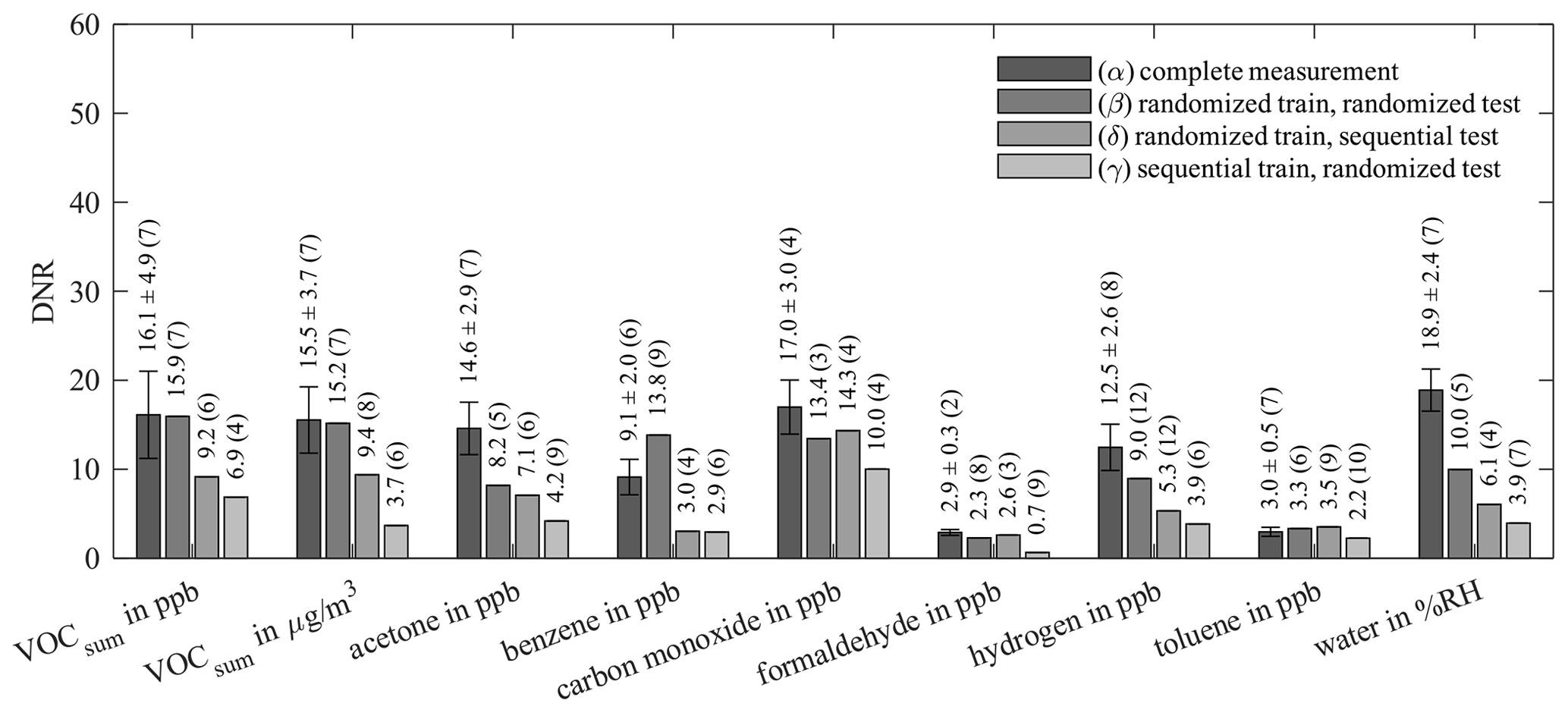
Figure 9Dynamic range (DNR) of AS-MLV-P2 for different training and testing models. All models use 10-fold cross-validation for hyperparameter optimization; the resulting number of PLSR components, determined with Eq. (2), is given in parentheses. A detailed description of (α)–(δ) is given in Table 4.
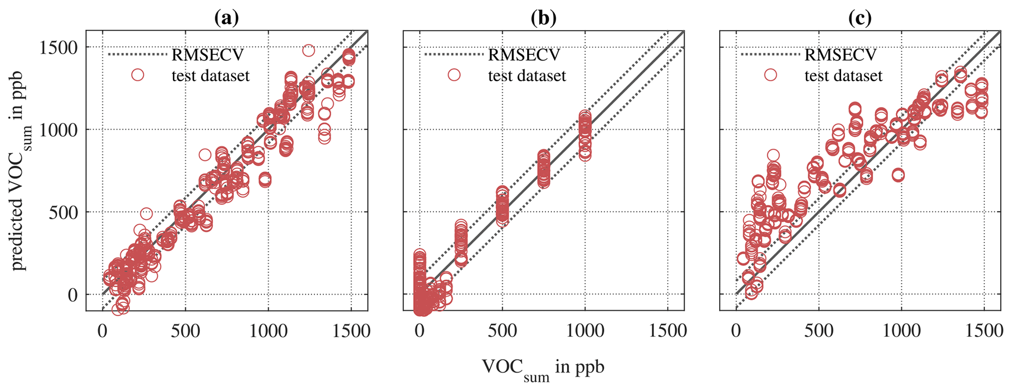
Figure 10PLSR models for AS-MLV-P2 for quantification of VOCsum in ppb for different training and testing models. (a) Randomized training and testing (Table 4, α). (b) Randomized training and sequential testing (Table 4, β). (c) Sequential training and randomized testing (Table 4, δ).
Figure 5 shows the R2 value for both AS-MLV and AS-MLV-P2 for different models. All models except the model for formaldehyde and toluene achieve an R2 over 0.86, and even over 0.94 with the exclusion of benzene. This indicates that a satisfying quantification of VOCsum and all gases except formaldehyde and toluene is possible with both sensors. The performance of the models is assessed with the RMSEP in Fig. 6 and the DNR in Fig. 7. Similar RMSEP values are achieved with both sensors for the different models. The regression models of AS-MLV and AS-MLV-P2 show the best performance for carbon monoxide with a DNR of 31. The regression models for acetone and hydrogen also achieve satisfactory results with a DNR between 16 and 18. The DNR for benzene with a value of 13 is relatively low considering the (unrealistically) high concentrations. The two gases with very low concentrations, toluene and formaldehyde, cannot be selectively quantified in this complex background, indicated by a DNR below 6. VOCsum can be quantified with a DNR of 18–19 independent of the unit (µg/m3 or ppb). This is interesting because the two dominating VOCs, acetone and benzene, represent different chemical classes and have a 30 % difference in molecular weight.
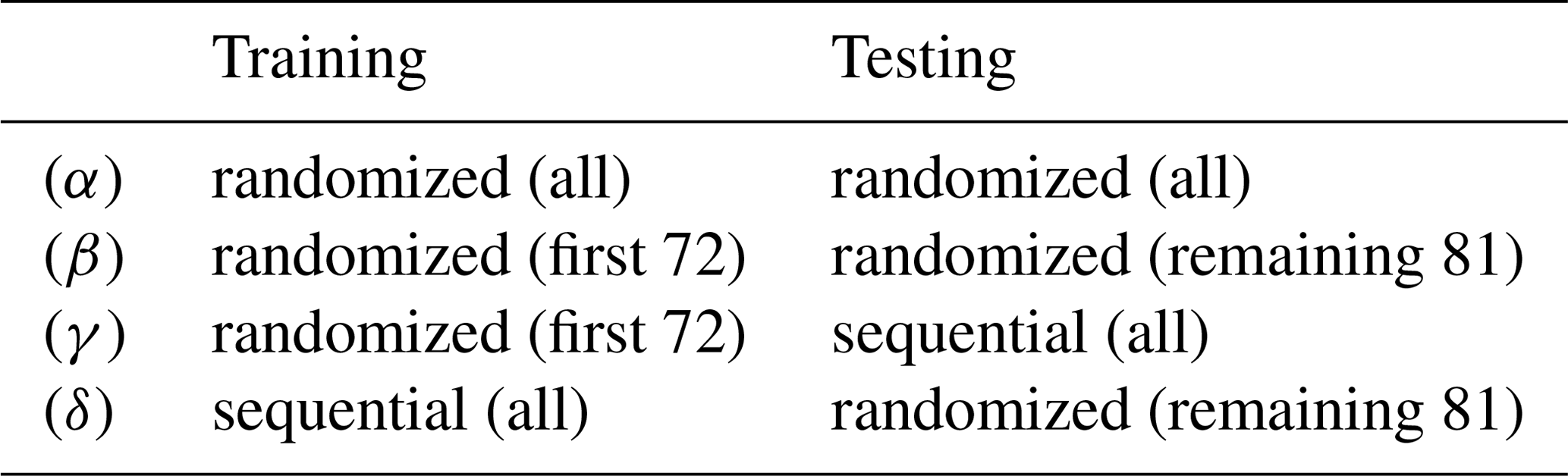
For a comparison between randomized and sequential calibration methods, we compare different combinations of training/validation and testing (Table 4). For compatibility, the randomized dataset with a higher concentration dynamic is reduced to a dataset in which all concentrations are in the range of 0–120 % of the sequential measurement, resulting in 153 gas exposures. The distribution of all gases and VOCsum is shown in Fig. A2. Since the last six gas exposures (75 %RH, 750 and 100 ppb benzene, all formaldehyde concentrations) are missing from the sequential dataset due to a technical error, there are 66 sequential gas mixtures in total. Combination (α) shows the evaluation of the reduced randomized dataset with 153 gas exposures. For the evaluation we used 10-fold nested cross-validation for hyperparameter optimization and testing like the evaluation in Figs. 6 and 7. We split the reduced dataset from the randomized measurement for combinations (β) to (δ) into two datasets. The first dataset contains the first 72 randomized gas exposures for training and hyperparameter optimization, and the second dataset the remaining 81 for testing. This allows us to compare randomized calibration with sequential testing and vice versa. The hyperparameter optimization during the training was always based on 10-fold cross-validation for randomized and sequential training.
Comparing the results of (α) and the previous evaluation in Figs. 6 and 7 shows the influence of reducing the randomized dataset for better compatibility with the sequential test scenario. The results of (α) and (β) show the influence of the two different evaluations. (γ) explores the prediction ability of a model trained with randomized data for sequential data, and (δ) vice versa. The performances of these four models are compared in Fig. 8 (RMSEP) and Fig. 9 (DNR) for the AS-MLV-P2. The AS-MLV shows similar results and can be found in Figs. C1 and C2. The RMSEPs of the models with randomized training (α) to (γ) are close together. The only exception is sequential testing – i.e., model (γ) – for benzene, producing a significantly larger RMSEP. The reverse case – i.e., model (δ) predicting randomized data after a sequential training – results in considerably larger RMSEPs in practically all cases. Despite the RMSEPs being similar for (α) to (γ) and Fig. 6, the DNR (Fig. 9) reveals the superiority of the results shown in Fig. 7 trained with a larger concentration range. The comparison between the randomized (β, γ) and sequential (δ) training of the reduced dataset only shows similar performance for carbon monoxide. The randomized data are obviously more challenging to predict and, at the same time, provide a better model with a higher DNR for prediction, which is to be expected due to the much larger variability of the background. At the same time, this allows for more efficient training closer to reality, since one data point is obtained for each gas from each gas mixture.
Table 4Combinations of training including hyperparameter optimization and testing datasets for a comparison between randomized and sequential calibration methods for the reduced dataset.
Comparing the PLSR models for VOCsum (in ppb) for combinations (β), (γ) and (δ) from Table 4 indicates that classical sequential calibration (see Fig. 10b) is a subset of the randomized calibration presented here (see Fig. 10a). The models trained with randomized mixtures in Fig. 10a and b show a slightly larger RMSECV compared to the sequential training shown in Fig. 10c. However, only these random models can accurately and precisely predict both the randomized and sequential dataset. The sequentially trained (and validated) model in Fig. 10c achieves a slightly lower RMSECV but fails to predict the more complex randomized dataset. Note that the measurement duration for both datasets is identical.
In this paper an efficient and effective gas sensor calibration based on randomized gas mixtures is presented. The results are compared with a classical calibration strategy based on individual gas exposures with sequentially increasing concentrations and fixed steps. While a model trained with data from the sequential calibration performs poorly in the more realistic case of complex gas mixtures, the novel randomized calibration achieves very promising results for all tested datasets, making it more effective. Since generating the required data with randomized gas mixtures does not take more time (and could, potentially, take considerably less for more targets) than the classical sequential calibration strategy, it is also more efficient. Our method was developed and tested with the real-world application of indoor air quality monitoring in mind and thus presents an important tool for the successful transfer of chemical sensors from the laboratory to the field. Its statistical nature makes it robust against overfitting and well suited for machine learning algorithms.
Since only single gases were measured sequentially in the study presented here, an investigation of the performance and stability of sequential calibrations with fully sampled combinations should follow for a more complete comparison to the randomized strategy. The aim of these investigations should be to determine the ideal number of randomized mixtures for obtaining a reliable model for predicting the concentration of an individual gas or a gas mixture. To check for generalizability, tests with different mixture compositions, for example by replacing one or two gases, will also be considered.
The six gases investigated in this work are probably not enough to fully characterize the performance of sensors for indoor air quality assessment, especially for a quantification of a single VOC. Therefore, the complexity, for example the number of backgrounds and interfering and target gases, should be rigorously increased in order to get closer to reality. A next step is the development of new gas mixing apparatus allowing a higher number of gases to be measured. By testing different distributions, efficiency and performance could be further improved. In addition, extensive field tests with reference analysis are necessary to demonstrate the advantage of the calibration strategy for real-world applications.
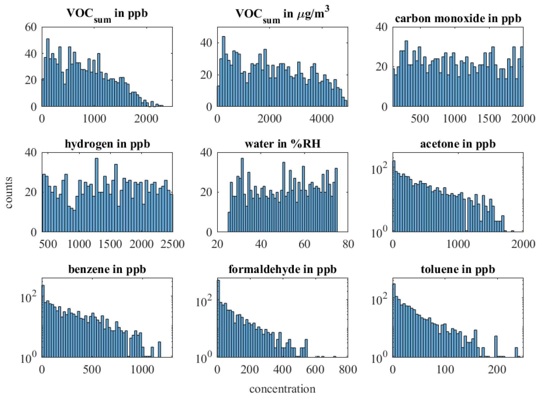
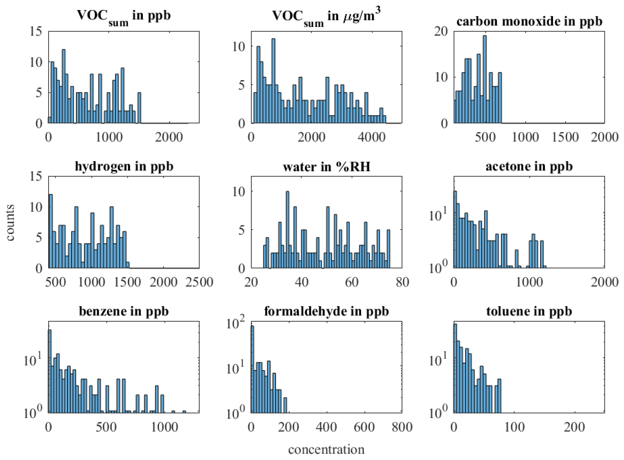
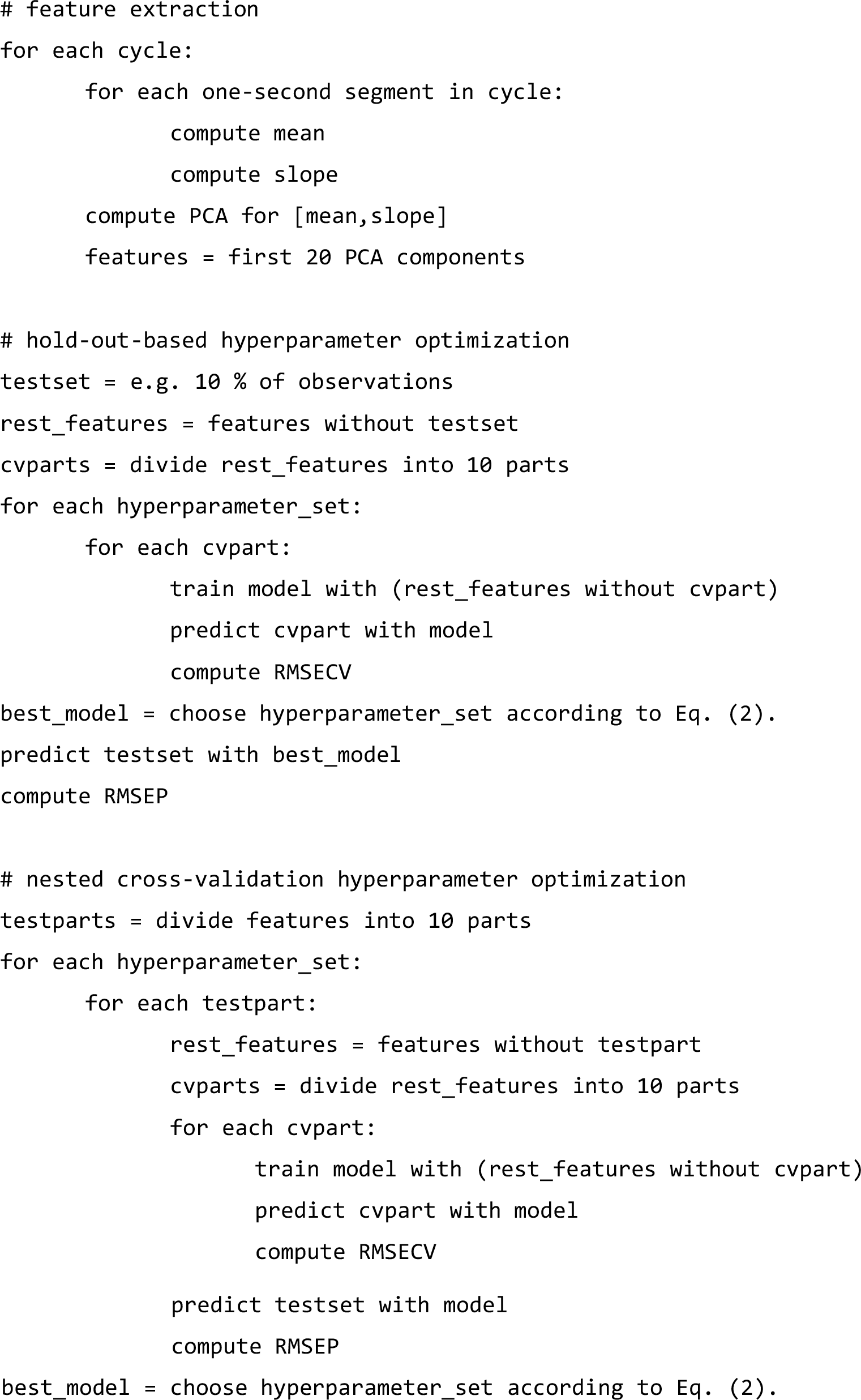
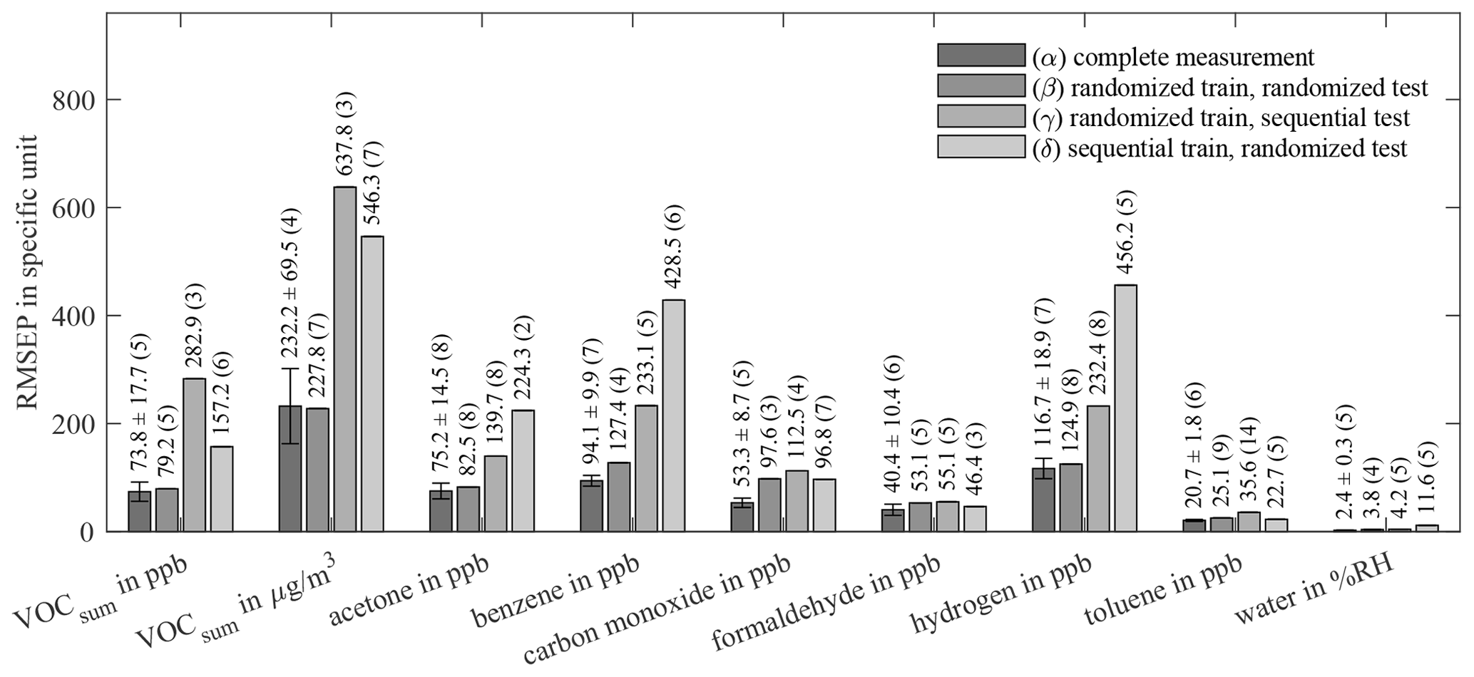
Figure C1Root-mean-square error of prediction (RMSEP) of AS-MLV for different training and testing models and targets. All models use 10-fold cross-validation for hyperparameter optimization; the resulting number of PLSR components, determined with Eq. (2), is given in parentheses. A detailed description of (α)–(δ) is given in Table 4.
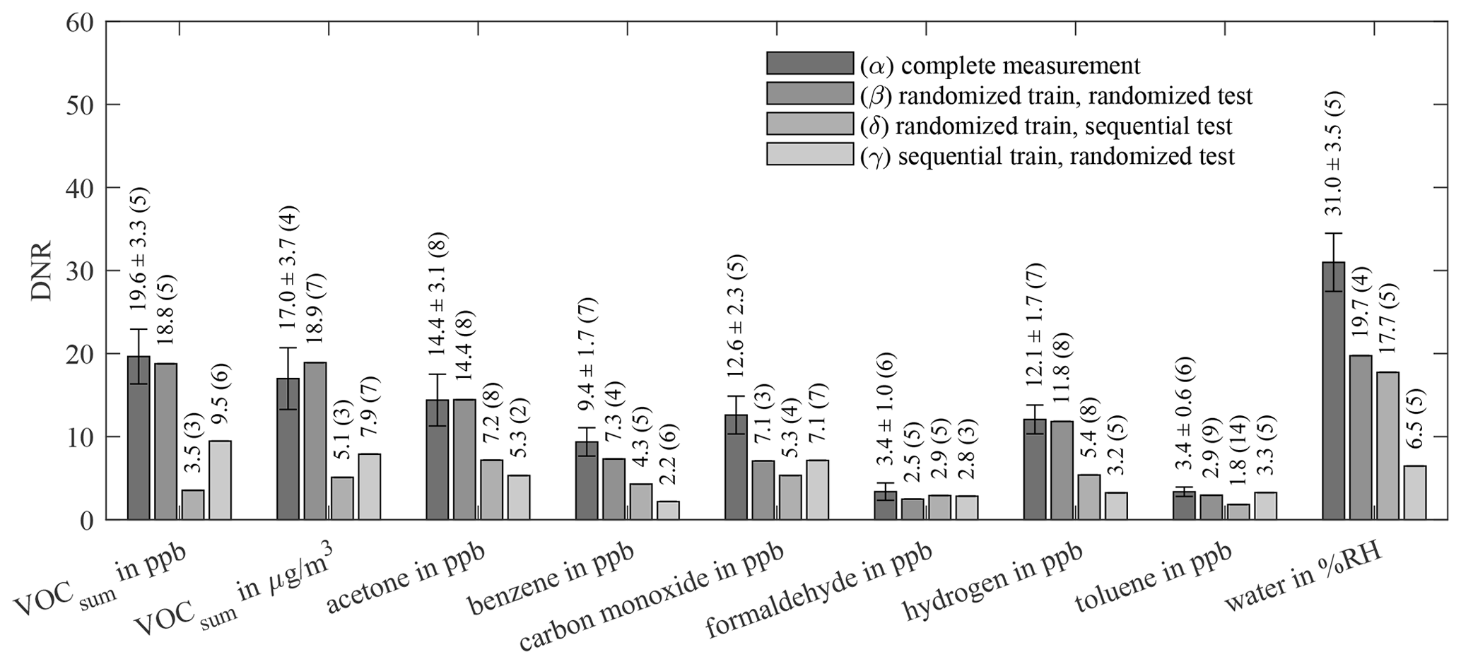
Figure C2Dynamic range (DNR) of AS-MLV for different training and testing models and targets. All models use 10-fold cross-validation for hyperparameter optimization; the resulting number of PLSR components, determined with Eq. (2), is given in parentheses. A detailed description of (α)–(δ) is given in Table 4.
The data presented in this article are stored in an internal system according to the guidelines of the German Research Foundation (DFG). The data for the evaluation can also be found at https://doi.org/10.5281/zenodo.4264224 (Baur et al., 2020).
TB, MB and CS conceptualized the project. TB and CS built the setup for the MOS sensors. MB wrote the software for the randomized calibration. TB and MB performed the measurements and evaluation. TB visualized the results and wrote with MB and CS the original draft of the paper. TS and AS reviewed and edited the paper.
The authors declare that they have no conflict of interest.
This article is part of the special issue “Dresden Sensor Symposium DSS 2019”. It is a result of the “14. Dresdner Sensor-Symposium”, Dresden, Germany, 2–4 December 2019.
We acknowledge support by the Deutsche Forschungsgemeinschaft (DFG, German Research Foundation) and Saarland University within the funding program Open Access Publishing.
This paper was edited by Winfried Vonau and reviewed by two anonymous referees.
Anon: Directive 2004/42/EC of the European Parliament and of the Council of 21 April 2004 on the limitation of emissions of volatile organic compounds due to the use of organic solvents in certain paints and varnishes and vehicle refinishing products and amendi, available at: https://eur-lex.europa.eu/eli/dir/2004/42/2019-07-26 (last access: 27 May 2020), 2004.
Anon: Beurteilung von Innenraumluftkontaminationen Mittels Referenz- und Richtwerten?: Handreichung der Ad-hoc-Arbeitsgruppe der Innenraumlufthygiene- Kommission des Umweltbundesamtes und der Obersten Landesgesundheitsbehörden, Bundesgesundheitsblatt – Gesundheitsforschung – Gesundheitsschutz, 50, 990–1005, https://doi.org/10.1007/s00103-007-0290-y, 2007.
Anon: Richtwert für Formaldehyd in der Innenraumluft, Bundesgesundheitsblatt – Gesundheitsforschung – Gesundheitsschutz, 595, 1040–1044, https://doi.org/10.1007/s00103-016-2389-5, 2016.
Bajtarevic, A., Ager, C., Pienz, M., Klieber, M., Schwarz, K., Ligor, M., Ligor, T., Filipiak, W., Denz, H., Fiegl, M., Hilbe, W., Weiss, W., Lukas, P., Jamnig, H., Hackl, M., Haidenberger, A., Buszewski, B., Miekisch, W., Schubert, J., and Amann, A.: Noninvasive detection of lung cancer by analysis of exhaled breath, BMC Cancer, 9, 348, https://doi.org/10.1186/1471-2407-9-348, 2009.
Bastuck, M.: Improving the Performance of Gas Sensor Systems with Advanced Data Evaluation, Operation, and Calibration Methods, Linköping University Electronic Press, Linköping, 2019.
Bastuck, M. and Fricke, T.: Temperature-modulated gas sensor signal, Zenodo, https://doi.org/10.5281/ZENODO.1411209, 2018.
Bastuck, M., Baur, T., Richter, M., Mull, B., Schütze, A., and Sauerwald, T.: Comparison of ppb-level gas measurements with a metal-oxide semiconductor gas sensor in two independent laboratories, Sens. Actuators, B, 273, 1037–1046, https://doi.org/10.1016/j.snb.2018.06.097, 2018a.
Bastuck, M., Baur, T., and Schütze, A.: DAV3E – a MATLAB toolbox for multivariate sensor data evaluation, J. Sens. Sens. Syst., 7, 489–506, https://doi.org/10.5194/jsss-7-489-2018, 2018b.
Baur, T., Schütze, A., and Sauerwald, T.: Optimierung des temperaturzyklischen Betriebs von Halbleitergassensoren, Tech. Mess., 82, 187–195, https://doi.org/10.1515/teme-2014-0007, 2015.
Baur, T., Schultealbert, C., Schütze, A., and Sauerwald, T.: Device for the detection of short trace gas pulses, Tech. Mess., 85, 496–503, https://doi.org/10.1515/teme-2017-0137, 2018a.
Baur, T., Schultealbert, C., Schütze, A., and Sauerwald, T.: Novel method for the detection of short trace gas pulses with metal oxide semiconductor gas sensors, J. Sens. Sens. Syst., 7, 411–419, https://doi.org/10.5194/jsss-7-411-2018, 2018b.
Baur, T., Bastuck, M., and Schultealbert, C.: Random gas mixtures for efficient gas sensor calibration: Dataset, Zenodo, https://doi.org/10.5281/zenodo.4264224, 2020.
Borrego, C., Costa, A. M., Ginja, J., Amorim, M., Coutinho, M., Karatzas, K., Sioumis, T., Katsifarakis, N., Konstantinidis, K., De Vito, S., Esposito, E., Smith, P., André, N., Gérard, P., Francis, L. A., Castell, N., Schneider, P., Viana, M., Minguillón, M. C., Reimringer, W., Otjes, R. P., von Sicard, O., Pohle, R., Elen, B., Suriano, D., Pfister, V., Prato, M., Dipinto, S., and Penza, M.: Assessment of air quality microsensors versus reference methods: The EuNetAir joint exercise, Atmos. Environ., 147, 246–263, https://doi.org/10.1016/j.atmosenv.2016.09.050, 2016.
Castell, N., Dauge, F. R., Schneider, P., Vogt, M., Lerner, U., Fishbain, B., Broday, D., and Bartonova, A.: Can commercial low-cost sensor platforms contribute to air quality monitoring and exposure estimates?, Environ. Int., 99, 293–302, https://doi.org/10.1016/j.envint.2016.12.007, 2017.
Fonollosa, J.: Gas sensor array under dynamic gas mixtures Data Set, UCI Machine Learning Repository, available at: https://archive.ics.uci.edu/ml/datasets/Gas+sensor+array+under+dynamic+gas+mixtures (last access: 31 March 2020), 2015.
Fonollosa, J.: Twin gas sensor arrays Data Set, UCI Machine Learning Repository, available at: https://archive.ics.uci.edu/ml/datasets/Twin+gas+sensor+arrays (last access: 31 March 2020), 2016.
Fonollosa, J., Rodríguez-Luján, I., and Huerta, R.: Chemical gas sensor array dataset, Data in Brief, 3, 85–89, https://doi.org/10.1016/j.dib.2015.01.003, 2015a.
Fonollosa, J., Rodríguez-Luján, I., Trincavelli, M., and Huerta, R.: Dataset from chemical gas sensor array in turbulent wind tunnel, Data in Brief, 3, 169–174, https://doi.org/10.1016/j.dib.2015.02.014, 2015b.
Fonollosa, J., Solórzano, A., Jiménez-Soto, J. M., Oller-Moreno, S., and Marco, S.: Gas sensor array for reliable fire detection, Procedia Engineer., 168, 444–447, https://doi.org/10.1016/j.proeng.2016.11.540, 2016.
Gramm, A. and Schütze, A.: High performance solvent vapor identification with a two sensor array using temperature cycling and pattern classification, Sens. Actuators, B, 95, 58–65, https://doi.org/10.1016/S0925-4005(03)00404-0, 2003.
Helwig, N., Schüler, M., Bur, C., Schütze, A., and Sauerwald, T.: Gas mixing apparatus for automated gas sensor characterization, Meas. Sci. Technol., 25, 055903, https://doi.org/10.1088/0957-0233/25/5/055903, 2014.
Hofmann, H. and Plieninger, P.: Bereitstellung einer Datenbank zum Vorkommen von flüchtigen organischen Verbindungen in der Raumluft, WaBoLu-Hefte, 5, 161, 2008.
Karagulian, F., Barbiere, M., Kotsev, A., Spinelle, L., Gerboles, M., Lagler, F., Redon, N., Crunaire, S., and Borowiak, A.: Review of the Performance of Low-Cost Sensors for Air Quality Monitoring, Atmosphere, 10, 506, https://doi.org/10.3390/atmos10090506, 2019.
Kohl, D., Kelleter, J., and Petig, H.: Detection of Fires by Gas Sensors, Sensors Updat., 9, 161–223, https://doi.org/10.1002/1616-8984(200105)9:1<161::AID-SEUP161>3.0.CO;2-A, 2001.
Leidinger, M., Schultealbert, C., Neu, J., Schütze, A., and Sauerwald, T.: Characterization and calibration of gas sensor systems at ppb level – a versatile test gas generation system, Meas. Sci. Technol., 29, 015901, https://doi.org/10.1088/1361-6501/AA91DA, 2018.
Levitt, M. D.: Production and excretion of hydrogen gas in man, The New England journal of medicine, 281, 122–127, https://doi.org/10.1056/NEJM196907172810303, 1969.
Lourenço, C. and Turner, C.: Breath Analysis in Disease Diagnosis: Methodological Considerations and Applications, Metabolites, 4, 465–498, https://doi.org/10.3390/metabo4020465, 2014.
Marco, S. and Gutierrez-Galvez, A.: Signal and data processing for machine olfaction and chemical sensing: A review, IEEE Sens. J., 12, 3189–3214, https://doi.org/10.1109/JSEN.2012.2192920, 2012.
Oehlert, G. W.: A First Course in Design and Analysis of Experiments, University of Minnesota Digital Conservancy, W. H. Freeman & Company, ISBN-10: 0-7167-3510-5, 2000.
Sauerwald, T., Baur, T., Leidinger, M., Reimringer, W., Spinelle, L., Gerboles, M., Kok, G., and Schütze, A.: Highly sensitive benzene detection with metal oxide semiconductor gas sensors – an inter-laboratory comparison, J. Sens. Sens. Syst., 7, 235–243, https://doi.org/10.5194/jsss-7-235-2018, 2018.
Schleyer, R., Bieber, E., and Wallasch, M.: Das Luftnetz des Umweltbundesamt, available at: https://www.umweltbundesamt.de/sites/default/files/medien/378/publikationen/das_luftmessnetz_des_umweltbundesamtes_bf_0.pdf (last access: 19 November 2020), 2013.
Schultealbert, C., Baur, T., Schütze, A., and Sauerwald, T.: Facile quantification and identification techniques for reducing gases over a wide concentration range using a MOS sensor in temperature-cycled operation, Sensors, 18, 744, https://doi.org/10.3390/s18030744, 2018a.
Schultealbert, C., Baur, T., Schütze, A., and Sauerwald, T.: Investigating the role of hydrogen in the calibration of MOS gas sensors for indoor air quality monitoring, Conference Proceedings Indoor Air, 15th Conference of the International Society of Indoor Air Quality & Climate, oral presentation, 22–27 July 2018, Philadelphia, PA, USA, 2018b.
Schütze, A. and Sauerwald, T.: Dynamic operation of semiconductor sensors, in: Semiconductor Gas Sensors, edited by: Jaaniso, R. and Tan, O. K., 385–412, Woodhead Publishing Series in Electronic and Optical Materials, 385–412, 2019.
Schütze, A., Baur, T., Leidinger, M., Reimringer, W., Jung, R., Conrad, T., and Sauerwald, T.: Highly Sensitive and Selective VOC Sensor Systems Based on Semiconductor Gas Sensors: How to?, Environments, 4, 20, https://doi.org/10.3390/environments4010020, 2017.
Seifert, B.: Richtwerte für die Innenraumluft Die Beurteilung der Innenraumluftqualität mit Hilfe der Summe der flüchtigen organischen Verbindungen (TVOC-Wert), Bundesgesundheitsblatt – Gesundheitsforschung – Gesundheitsschutz, 42, 270–278, https://doi.org/10.1007/s001030050091, 1999.
Sharma, B., Sharma, A., and Kim, J. S.: Recent advances on H2 sensor technologies based on MOX and FET devices: A review, Sens. Actuators, B, 262, 758–770, https://doi.org/10.1016/j.snb.2018.01.212, 2018.
Spinelle, L., Gerboles, M., Kok, G., Persijn, S., and Sauerwald, T.: Review of Portable and Low-Cost Sensors for the Ambient Air Monitoring of Benzene and Other Volatile Organic Compounds, Sens, 17, 1520, https://doi.org/10.3390/s17071520, 2017.
Stone, M.: Cross-Validatory Choice and Assessment of Statistical Predictions, J. Roy. Stat. Soc. B Met., 36, 111–133, https://doi.org/10.1111/j.2517-6161.1974.tb00994.x, 1974.
Sundgren, H., Winquist, F., Lukkari, I., and Lundstrom, I.: Artificial neural networks and gas sensor arrays: quantification of individual components in a gas mixture, Meas. Sci. Technol., 2, 464, https://doi.org/10.1088/0957-0233/2/5/008, 1991.
Tomchenko, A. A., Harmer, G. P., and Marquis, B. T.: Detection of chemical warfare agents using nanostructured metal oxide sensors, Sensor. Actuat. B-Chem., 108, 41–55., 2005.
Tomlin, J., Lowis, C., and Read, N. W.: Investigation of normal flatus production in healthy volunteers, Gut, 32, 665–669, https://doi.org/10.1136/gut.32.6.665, 1991.
WHO Regional Office for Europe: WHO guidelines for indoor air quality: selected pollutants, Copenhagen, available at: https://www.ncbi.nlm.nih.gov/books/NBK138705/ (last access: 19 November 2020), 2010.
Wolfrum, E. J., Meglen, R. M., Peterson, D., and Sluiter, J.: Calibration transfer among sensor arrays designed for monitoring volatile organic compounds in indoor air quality, IEEE Sens. J., 6, 1638–1643, https://doi.org/10.1109/JSEN.2006.884558, 2006.
Yu, C., Hao, Q., Saha, S., Shi, L., Kong, X., and Wang, Z. L.: Integration of metal oxide nanobelts with microsystems for nerve agent detection, Appl. Phys. Lett., 86, 1–3, https://doi.org/10.1063/1.1861133, 2005.
Zhang, L., Tian, F., Liu, S., Guo, J., Hu, B., Ye, Q., Dang, L., Peng, X., Kadri, C., and Feng, J.: Chaos based neural network optimization for concentration estimation of indoor air contaminants by an electronic nose, Sensor. Actuat. A-Phys., 189, 161–167, https://doi.org/10.1016/j.sna.2012.10.023, 2013.
The term “contamination” here refers to observations used in the training of a model “spilling” or “leaking” into datasets used for validation or testing. Predicting observations used in the training usually results in deceivingly better model performance.
The definition of “good” in this context is arbitrary. We defined it as a model with an average error less than the minimum achieved error at any number of components plus 1 standard deviation.
- Abstract
- Motivation
- Experimental
- Results and discussion
- Conclusion and outlook
- Appendix A: Appendix A: Histogram of the complete and reduced dataset
- Appendix B: Pseudocode for data evaluation
- Appendix C: Results of the AS-MLV for comparison between randomized and sequential calibration
- Data availability
- Author contributions
- Competing interests
- Special issue statement
- Acknowledgements
- Review statement
- References