Influence of synchronization within a sensor network on machine learning results

Process sensor data allow for not only the control of industrial processes but also an assessment of plant conditions to detect fault conditions and wear by using sensor fusion and machine learning (ML). A fundamental problem is the data quality, which is limited, inter alia, by time synchronization problems. To examine the influence of time synchronization within a distributed sensor system on the prediction performance, a test bed for end-of-line tests, lifetime prediction, and condition monitoring of electromechanical cylinders is considered. The test bed drives the cylinder in a periodic cycle at maximum load, a 1 s period at constant drive speed is used to predict the remaining useful lifetime (RUL). The various sensors for vibration, force, etc. integrated into the test bed are sampled at rates between 10 kHz and 1 MHz. The sensor data are used to train a classification ML model to predict the RUL with a resolution of 1 % based on feature extraction, feature selection, and linear discriminant analysis (LDA) projection. In this contribution, artificial time shifts of up to 50 ms between individual sensors' cycles are introduced, and their influence on the performance of the RUL prediction is investigated. While the ML model achieves good results if no time shifts are introduced, we observed that applying the model trained with unmodified data only to data sets with time shifts results in very poor performance of the RUL prediction even for small time shifts of 0.1 ms. To achieve an acceptable performance also for time-shifted data and thus achieve a more robust model for application, different approaches were investigated. One approach is based on a modified feature extraction approach excluding the phase values after Fourier transformation; a second is based on extending the training data set by including artificially time-shifted data. This latter approach is thus similar to data augmentation used to improve training of neural networks.

1 Introduction

In the Industry 4.0 paradigm, industrial companies have to deal with several emerging challenges of which digitalization of the factory is one of the most important aspects for success. In digitalized factories, sometimes also referred to as “Factories of the Future” (FoF), the “Industrial Internet of Things” (IIoT) forms the networking basis and allows users to improve operational effectiveness and strategic flexibility (Eichstädt, 2020; Schütze et al., 2018). Key components of FoF and IIoT are intelligent sensor systems, also called cyber-physical systems, and machine learning (ML), which allow for the automation and improvement of complex process and business decisions in a wide range of application areas. For example, smart sensors can be used to evaluate the state of various components, determine the optimum maintenance schedule, or detect fault conditions (Schneider et al., 2018b), as well as to control entire production lines (Usuga Cadavid et al., 2020). To make full use of the wide-ranging potential of smart sensors, the quality of sensor data has to be taken into account (Teh et al., 2020). This is limited by environmental factors, sensor failures, measurement uncertainty, and – especially in distributed sensor networks – by time synchronization errors between individual sensors. Confidence in ML algorithms and their decisions or predictions requires reliable data and therefore a metrological infrastructure allowing for an assessment of the data quality. In this contribution, a software toolbox for statistical machine learning (Schneider et al., 2017, 2018b; Dorst et al., 2021a) is used to evaluate large data sets from distributed sensor networks under the influence of artificially generated time shifts to simulate synchronization errors. One aspect to address time synchronization problems in distributed sensor networks is improved time synchronization methods to provide a reliable global time for all sensors. Many different synchronization methods are proposed for sensor networks (Sivrikaya and Yener, 2004). However, improved time synchronization might not be possible or be too costly, especially in existing sensor networks which were often never designed for sensor data fusion, so the ML approach can be improved to achieve a more robust model with acceptable results as demonstrated in this contribution.

2 Test bed for data acquisition

Predictive maintenance, based on reliable condition monitoring, is a requirement for reducing repair costs and machine downtime and, as a consequence, increasing productivity. Therefore, an estimation of the remaining useful lifetime (RUL) of critical components is required. Since we are using a data-driven model, this cannot be done directly without reference data. A test bed for electromechanical cylinders (EMCs) with a spindle drive equipped with several sensors is used. This specific test bed was used as it contains a large variety of sensor domains and allows for physical interpretation. Because most industrial ML problems only use a subset of these sensors, the approaches of the chosen test bed can be transferred. In this test bed, long-term speed driving and high load tests are carried out until a position error of the EMC occurs, i.e., until the device under test (DUT) fails. Characteristic signal patterns and relevant sensors can be identified for condition monitoring as well as for RUL estimation of the EMCs. Figure 1 shows the scheme of the test bed. Simplified, the setup of the test bed consists of the tested EMC and a pneumatic cylinder which simulates the variable load on the EMC in axial direction. All parameters of the working cycle can be set by using a LabVIEW GUI.

Figure 1 Basic scheme of the EMC test bed (Helwig et al., 2017).

A typical working cycle lasts 2.8 s. It consists of a forward stroke and a return stroke of the EMC as well as a waiting time of 150 ms between both linear movements. The movements are always carried out with approximately maximum speed and maximum acceleration. The stroke range of the EMC is between 100 and 350 mm in the test bed. The combination of high travel speed (200 mm s⁻¹), high axial force (7 kN), and high acceleration (5 mm s⁻²) leads to fast wear of the EMC. The error criterion for failure of the EMC is defined as a too large deviation between the nominal and actual position values; i.e., the test is stopped as soon as the specified position accuracy (position accuracy < 30 mm) is no longer fulfilled due to increased friction.

To gather as much data as possible from different sensor domains for a comprehensive condition monitoring, the following 11 sensors are used within the test bed (Schneider et al., 2018a):

• one microphone with a sampling rate of 100 kHz;

• three accelerometers with 100 kHz sampling rate, attached at the plain bearing, at the piston rod, and at the ball bearing;

• four process sensors (axial force, pneumatic pressure, velocity, and active current of the EMC motor) with 10 kHz sampling rate each;

• three electrical motor current sensors with 1 MHz sampling rate each.

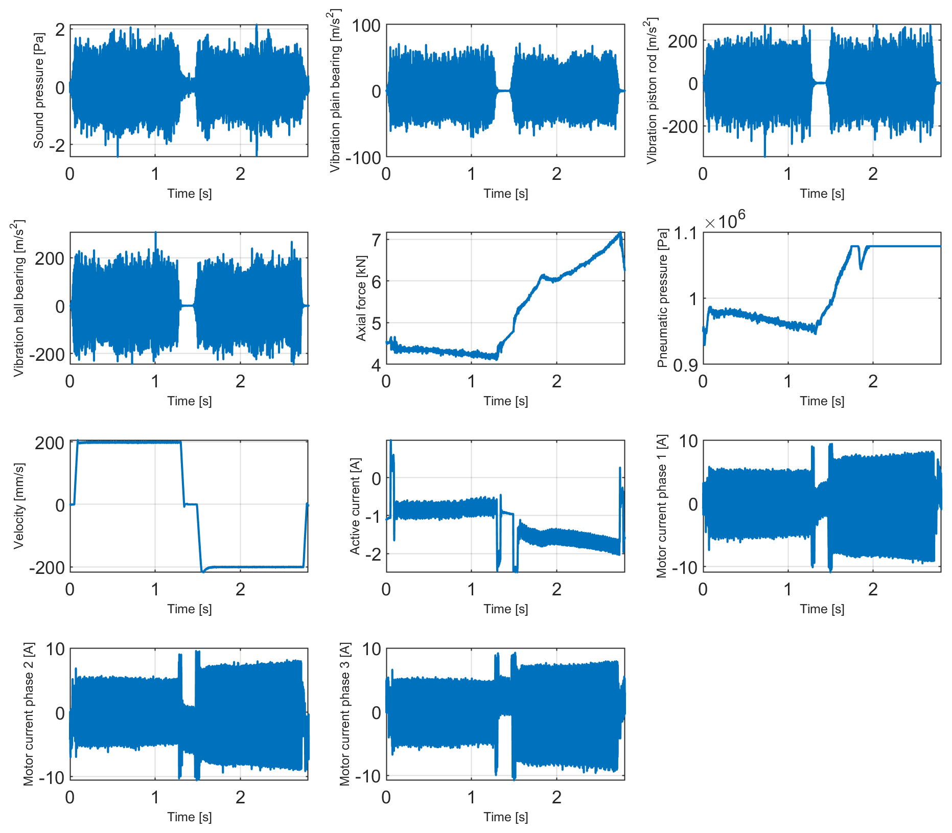
In Fig. 2, the raw data for one cycle and all sensors is shown. The collected data reflect the functionality of the EMC and its decrease during the long-term test. For data analysis, which is described in more detail in the next section, various EMCs were tested until the position error occurred. The typical lifetime of an EMC under these test conditions was approx. 629 000 cycles corresponding to roughly 20 d and generated an average of 12 TB of raw data.

Figure 2 Raw data recorded during one cycle by 11 sensors expressed in SI units.

3 ML toolbox for data analysis

The ML toolbox developed by Schneider et al. (2018b) is used for RUL analysis in this contribution. It can be applied in a fully automated way, i.e., without expert knowledge and without a detailed physical model of the process. After acquisition of the raw data, feature extraction and selection as well as classification and evaluation are performed, as shown in Fig. 3.

Figure 3 Schematic of the automatic toolbox for condition monitoring using machine learning, adapted from Dorst et al. (2019).

3.1 Feature extraction

In the beginning, unsupervised feature extraction (FE) is performed, i.e., without knowledge of the group to which the individual work cycle belongs, in this case the current state of aging (RUL). Features are generated from the repeating working cycles of the raw data. As there is no method that works well for all applications, features are extracted from different domains by five complementary methods:

• Adaptive linear approximation (ALA) divides the cycles into approximately linear segments. For each linear segment, mean value and slope are extracted as features from the time domain (Olszewski et al., 2001).

• Using principal component analysis (PCA), projections on the principal components are determined and used as features, representing the overall signal (Wold et al., 1987).

• The best Fourier coefficient (BFC) method extracts the 10 % of amplitudes with the highest average absolute value over all cycles and their corresponding phases as features from the frequency domain (Mörchen, 2003).

• The best Daubechies wavelet (BDW) algorithm is based on a wavelet transform, and as for BFC, the 10 % of the wavelet coefficients with the highest average absolute value over all cycles are chosen as features from the time-frequency domain.

• In general, information is also included in the statistical distribution of the measurement values. These features are extracted from a fixed number of equally sized segments of a cycle by the four statistical moments (SMs) of mean, variance, skewness, and kurtosis.

The objective of FE is to concentrate information in as few features as possible whilst achieving a precise prediction of the RUL. The FE methods are applied to all sensor signals and all cycles. This results in five feature sets with a large number of features in each. However, the number of features is still too high after performing feature extraction for Big Data applications, such as RUL estimation of the EMC as described in the previous section. Due to the insufficient data reduction in this step, feature selection is carried out with the extracted features to prevent the “curse of dimensionality” (Beyer et al., 1999).

3.2 Feature selection

Feature selection (FS) is a supervised step; i.e., the group to which each cycle belongs is known. In the case of the RUL estimation of the EMC, the target value is the used lifetime with a resolution of 1 %. As for feature extraction, no method alone can provide the optimum solution for all applications, so three different complementary methods are used for feature selection in the ML toolbox:

• Recursive Feature Elimination Support Vector Machine (RFESVM) uses a linear support vector machine (SVM) to recursively remove the features with the smallest contribution to the group separation from the set of all features (Guyon and Elisseeff, 2003; Rakotomamonjy, 2003).

• The RELIEFF algorithm is used when the groups cannot be separated linearly. This algorithm finds the nearest hits and nearest misses for each point by using k-nearest neighbors with the Manhattan norm (Kononenko and Hong, 1997; Robnik-Šikonja and Kononenko, 2003).

• Pearson correlation is used as a third method for feature (pre)selection because of its low computational cost. The features are sorted by their correlation coefficient to the target value. This coefficient indicates how large the linear correlation between a feature and the target value is.

Preselection based on Pearson correlation is performed to reduce the feature set to only 500 features before applying the RFESVM or RELIEFF algorithms to reduce the computational costs. After ranking the features with a feature selection algorithm, a 10-fold cross-validation (explained later) is carried out for every number of features to find the optimum number of features. Thus, the most relevant features with respect to the classification task are selected, and features with redundant or no information content are removed from the feature set.

In addition to reducing the data set, this step also avoids overfitting, which often occurs when the number of data points for developing the classification model is not significantly greater than the number of features.

3.3 Classification

The classification is carried out in two steps: a further dimensionality reduction followed by the classification itself. The further dimensionality reduction is based on linear discriminant analysis (LDA). It performs a linear projection of the feature space into a g−1-dimensional subspace for g groups which represent the corresponding system state. The intraclass variance, the variance within the classes, is minimized while the interclass variance, the variance between the classes, is maximized (Duda et al., 2001). Thus, the distance calculation in the classification step has only a complexity of g−1. The actual classification is carried out using the Mahalanobis distance; see Eq. (1):

$$\begin{array}{}\text{(1)}& d_{\mathrm{Mahal}}\left(\mathit{x}\right)=\sqrt{(\mathit{x}-\mathit{m}{)}^{\top }{\mathbf{S}}^{-\mathrm{1}}(\mathit{x}-\mathit{m})}.\end{array}$$

Here x denotes the vector of the test data, m the component-wise arithmetic mean, and S the covariance matrix of the group. For each data point, the Mahalanobis distance indicates how far it is away from the center of the data group, taking the group scattering into account. In order to classify the data, each sample is labeled with the class that has the smallest Mahalanobis distance. Points of equal Mahalanobis distance from a center graphically form a hyperellipse in the g−1-dimensional LDA space.

3.4 Evaluation

The k-fold stratified cross-validation (CV) is used for evaluation (Kohavi, 1995). This means the data set is randomly divided into k subsets, with k∈ℕ. Stratified means that each of the k subsets has approximately the same class distribution as the whole feature set. In the ML toolbox, k is usually set to 10. Thus, one group forms the test data set and nine groups form the training data set, from which the ML model is generated.

3.5 Automated ML toolbox

The automatic ML toolbox compares the 15 combinations that are achieved by combining all feature extraction methods and all selection methods. The cross-validation error, i.e., the percentage of misclassified cycles by the 10-fold cross-validation, is automatically calculated for each of the 10 permutations resulting from the 10-fold cross-validation and for each of the 15 FE/FS combinations. To compare the result of the different combinations, the mean of the 10 cross-validation errors (one cross-validation error per fold) per combination is used. The minimum value of all the 15 cross-validation errors (one error per combination) leads to the best combination of FE/FS method. Thus, finding the best combination of one feature extraction and one feature selection method for the current application case is a fully automated process that is performed offline. The actual classification is then carried out online by using only the best of the 15 combinations, which results in a low computational effort during application.

4 Application of the ML toolbox on test bed data

The basis for this contribution is a lifetime test of an EMC which originally lasted 20.4 d and consists of 629 485 cycles. Only 1 s of the synchronous phase of the return stroke (duration 1.2 s) for each working cycle is evaluated with the ML toolbox. During this 1 s period, the velocity is constant and the load is highest as the EMC is pulling against a constant load provided by the pneumatic cylinder; see Fig. 4. Thus, this 1 s period is suitable for ML problems.

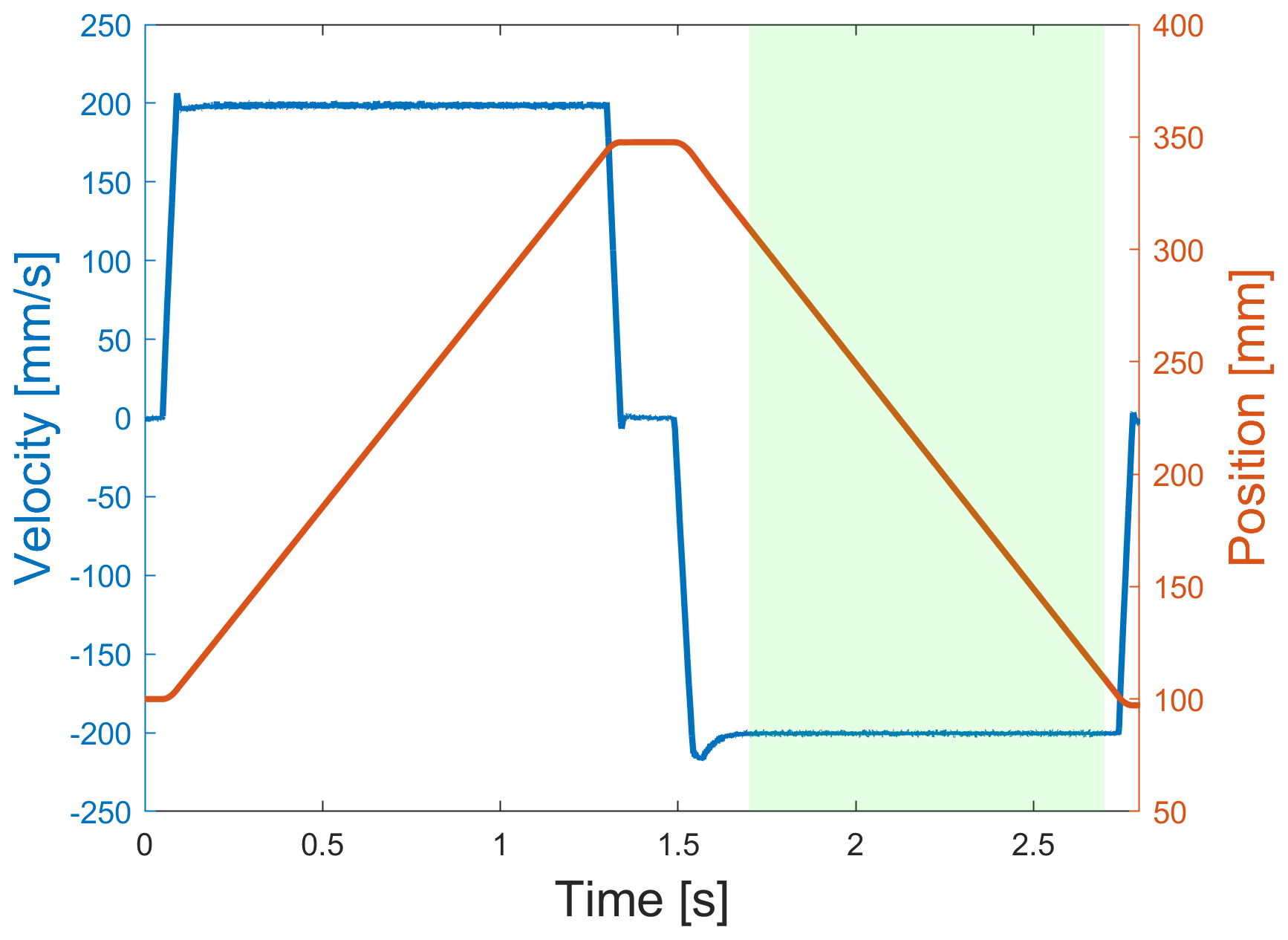
Figure 4 Working cycle depicted as position (red) and velocity (blue) consisting of forward stroke, waiting time, and return stroke, as well as the period (green) evaluated for estimation of the RUL.

For this full data set, where all sensors have their original sampling rate, the minimum cross-validation error of 8.9 % was achieved with 499 features and a combination of BFC and Pearson correlation together with the previously described LDA classifier (Schneider et al., 2018c). Pearson correlation was only used as selector due to the high computational time of RFESVM and RELIEFF for the full data set with 629 485 cycles. Feature extraction together with feature selection leads to a data reduction of approximately a factor of 60 000 in this case; i.e., the originally recorded 12 TB of raw data for this EMC is reduced to a feature set of approximately 200 MB.

To reduce computational costs and to allow us to study various influencing factors on the classification performance, a reduced data set with only every hundredth cycle is used in this contribution. A further reduction of the computational costs could be achieved by reducing the sampling rate of the data. To test the influence of lower sampling rates, several data sets with different sampling rates are used, and it can be observed that the best results across all used sampling rates are always achieved with a combination of BFC and RFESVM. As shown in Fig. 5, the minimum 10-fold cross-validation error of the EMC data sets with sampling rates of 1 kHz and more is nearly the same. Thus, the quality of the prediction is not influenced by a lower sampling rate. The minimum cross-validation error (18.15 %) is achieved with the 5 kHz data set, but with the 2 kHz version, the cross-validation error increases only slightly in the second decimal place (18.18 %). Thus, it is not necessary to use a data set with a higher sampling rate, and due to less computational costs, the 2 kHz data set is chosen for this contribution. It seems that several relevant features are in the range between 250 Hz and 1 kHz and, based on the Nyquist criterion, are thus contained in this data set. All further results in this contribution are based on the 2 kHz resolution data set of an EMC with 6292 cycles (1.1 GB) and time-shifted versions of this data set. The 2 kHz raw data set is available online for further analysis (Dorst, 2019).

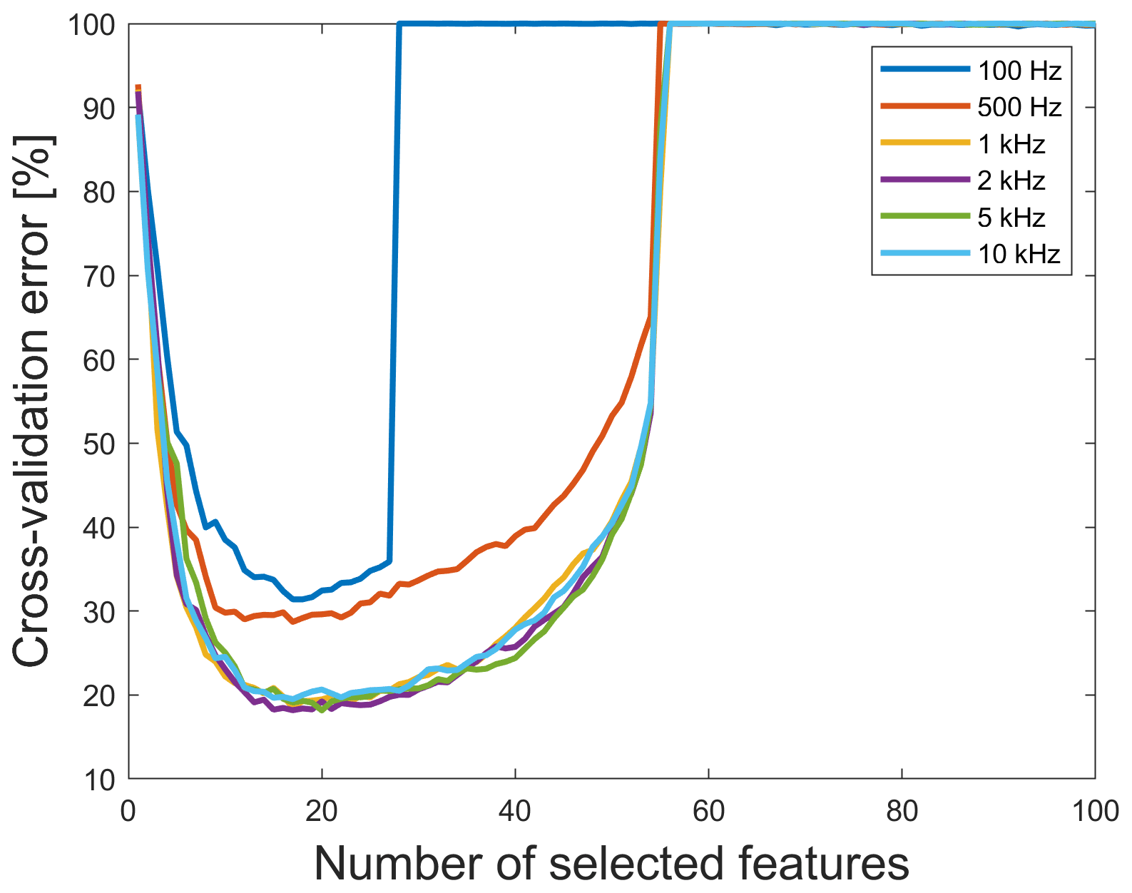
Figure 5 The 10-fold cross-validation error vs. number of selected features for data sets with different sampling rate using BFC as extractor and RFESVM as selector.

For this data set, the lowest cross-validation error is reached with features extracted from the frequency domain with BFC and RFESVM as selector. The cross-validation error for the 15 FE/FS combinations can be found in Table 1.

Table 1 Cross-validation error for different FE/FS combinations.

The lowest cross-validation error with 18.18 % misclassifications occurs when using only 17 features as shown in Fig. 6. The large increase of the cross-validation error when using 54–56 features or more in Figs. 5 and 6 can be understood considering the covariance matrices S used for calculation of the Mahalanobis distance. These covariance matrices have a reciprocal condition number of about 10⁻¹⁹ in 1-norm, which means that they are ill-conditioned. A reason for the ill-conditioned covariance matrices is the low number of cycles (only 62, which results from the 1 % resolution of the RUL together with 6292 cycles) per target class and the nearly equal number of features.

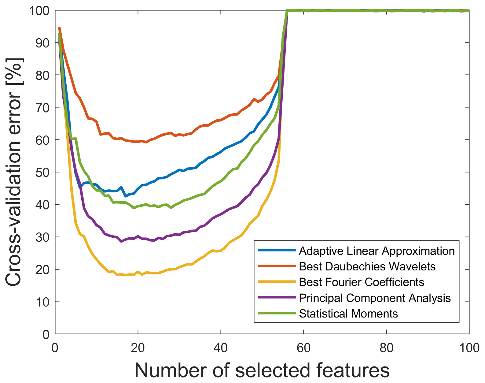
Figure 6 The 10-fold cross-validation error vs. number of selected features for the original 2 kHz data set without time shift using RFESVM as selector. For a better visibility, only results with RFESVM as selector are shown.

Since 11 sensors are used within the test bed, Fig. 7 shows which sensors are contributing to the 17 most important features for the RUL prediction using BFC as the feature extractor and RFESVM as selector. It can be clearly seen that five features each (i.e., 29 %) are derived from the microphone and the active current data. For further analysis, it is important to note that 12 of the 17 best Fourier coefficient features represent amplitudes.

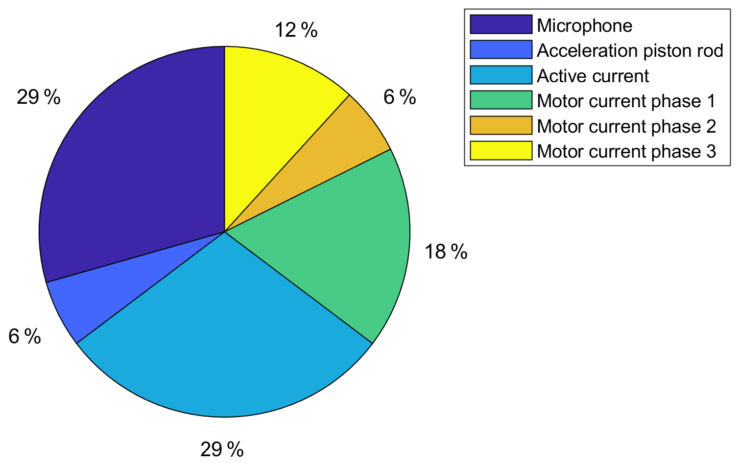
Figure 7 The 17 most important features by sensors, selected with RFESVM. Only 6 of the 11 sensors contribute to the 17 most important features.

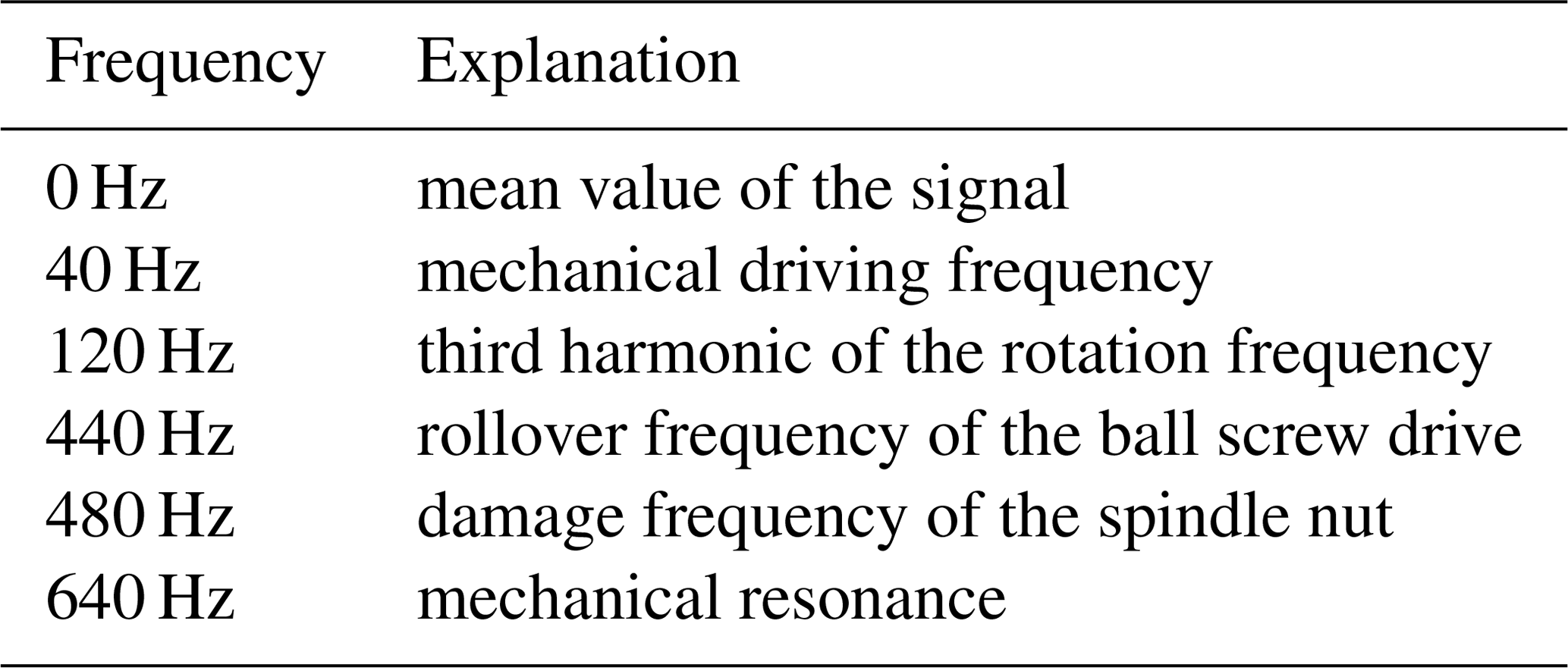
To check the plausibility of the results, Fig. 8 shows that these 17 most relevant features are within the range 0 to 640 Hz. Thus, using the 1 kHz data set would lead to a loss of relevant features (640 Hz). The dominant frequency here is 120 Hz (five features) which represents the third harmonic of the rotation frequency. The explanation for the other frequencies can be found in Table 2 (cf. Helwig, 2018).

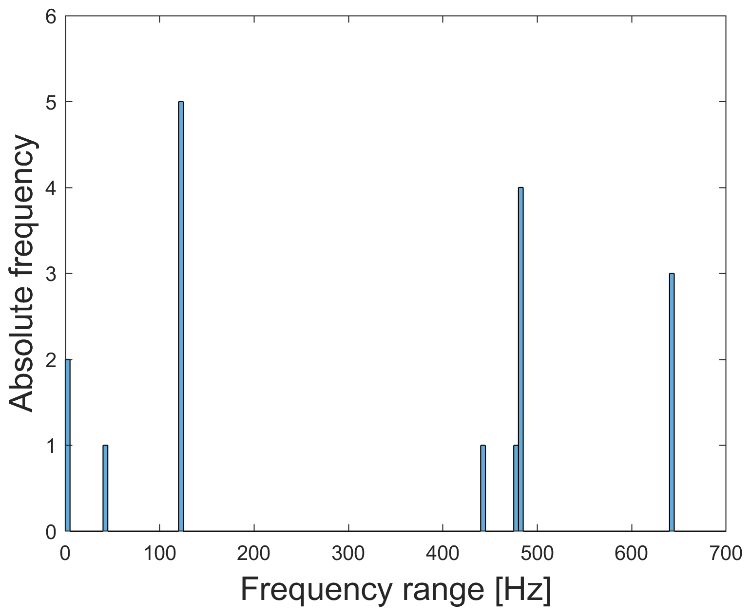
Figure 8 Frequency range of the 17 most relevant features. The frequencies of all relevant features are ≤640 Hz.

Table 2 Explanation of the frequencies of the 17 most relevant features. The 17 most relevant features are physically explainable.

5 Synchronization problems and their effects on machine learning results

Synchronization between different sensors is important to enable data analysis. Correctly performed data fusion is crucial for applications, e.g., in industrial condition monitoring (Helwig, 2018). Synchronization problems there simply means that the raw data of the sensors' cycles are shifted against each other. The feature extraction is carried out for every sensor and all features are packed together in the classifier. As the temporal localization of effects can play a role in ML, synchronization problems can lead to poor classification results like later shown in this contribution.

To analyze the effects of synchronization problems between the individual sensors installed within the test bed and their effect on the lifetime prognosis, time-shifted data sets downsampled to 2 kHz are used. Thereby, the raw data set with full resolution, mentioned in Sect. 4, serves as basis to simulate synchronization errors. These errors are simulated by manipulating the raw data set with random time shifts between the individual sensors' cycles in the 1.0 s window of the return stroke. The maximum time shift of a cycle is ±50 ms in relation to the original time axis to ensure that only data from the return stroke are used for all sensors. The minimal possible time shift is ±0.1 ms as the lowest sampling rate over all sensors is 10 kHz.

Clock synchronization is a topic of research still today (Yiğitler et al., 2020). As shown in this contribution, it is important to think about clock synchronization, because if not, then there will be serious issues with the results. For distributed sensor networks, the considered time shifts are in a range that can be expected (Tirado-Andrés and Araujo, 2019).

After simulating these errors with the raw data set, the different time-shifted data sets are downsampled to 2 kHz to reduce computational complexity. Analysis is carried out using time-shifted data sets with a minimum of ±0.1 ms per cycle (based on the time axis of the 2 kHz raw data set) and sensor up to a maximum of ±50 ms per cycle and sensor. The time-shifted values in every cycle for every sensor are randomly generated with a discrete uniform distribution. This means that the time shift for all samples of one single cycle is the same but not for the same cycle over all sensors. The best combination of FE/FS algorithm for all five time-shifted data sets is BFC as extractor together with RFESVM as selector. An increase in the cross-validation error is observed with increasing random time shifts for all sensors (cf. Table 3). For random time shifts between 0.1 and 1 ms, the cross-validation error is nearly the same; the change is only in the first decimal place. Using random time shifts with more than ±50 ms leads to a significant decrease of the classification performance. A likely reason for this decrease is probably that not only data from the synchronous phase of the return stroke are used, but also some data from the acceleration or deceleration phase of the return stroke are included in the evaluated 1 s period. To depict the effect of increasing random time shifts on the prediction performance more clearly, the cross-validation error using BFC as extractor, RFESVM as selector, and time shifts from 0.1 to 50 ms between all 11 sensors are shown in Fig. 9 vs. the number of features. Every model was trained with the specific time-shifted data set. It can be clearly seen that small time shifts only have a minor effect on the cross-validation error, whereas time shifts of 1 ms or more increase the cross-validation error noticeably. One reason is that the variance in the data increases by increasing random time shifts and makes it harder for the model to learn. For constant time shifts, on the other hand, the cross-validation error is nearly the same as for the raw data set (cf. Fig. 10), because every cycle is shifted by the same constant time, which does not affect the Fourier coefficients. Although, random time shifts have no influence on the amplitude spectrum in theory, but because of the experimental setup, there can occur cross-influences that make model building harder.

Table 3 Cross-validation error for the 2 kHz raw data set and 2 kHz data sets with different time shifts with BFC as extractor and RFESVM as selector.

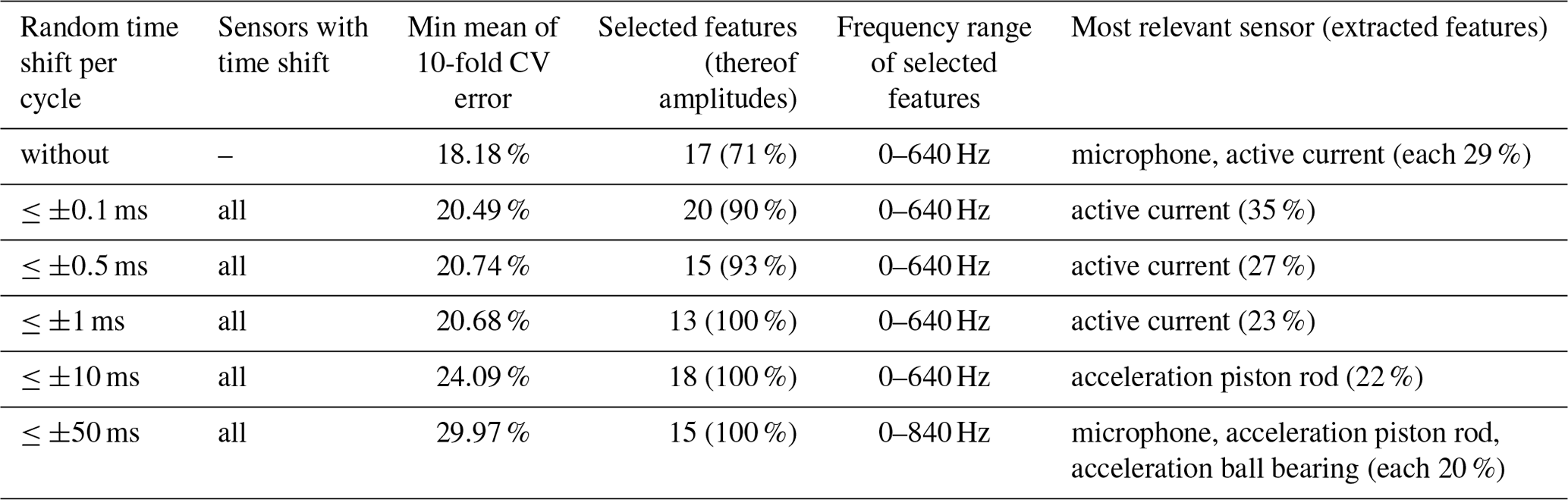
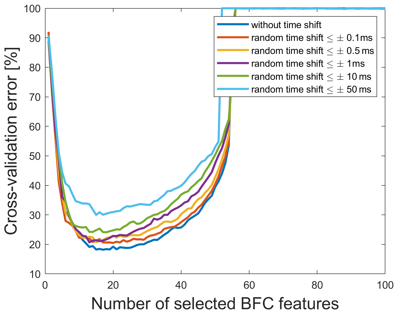
Figure 9 Cross-validation errors vs. the number of selected BFC features for different random simulated synchronization errors using RFESVM as selector.

Figure 10 Cross-validation errors vs. the number of selected BFC features for constant shifted time windows with RFESVM as selector.

Since most of the results resulting from time-shifted data sets are almost equivalent to those obtained for the 2 kHz raw data set, not all results are explicitly discussed in this contribution. Only the data set with time shifts of maximum ±50 ms for all sensors' cycles is considered in more detail here. On the one hand, this time shift is the maximum possible when taking into account the cycle length of 2.8 s and evaluating a full second of the return stroke, and on the other hand, this time shift provides the worst cross-validation error for the combination of BFC and RFESVM. As shown in Fig. 11, the minimum cross-validation error is now 29.97 %, which is significantly worse than for the original data set without time shifts (18.18 %).

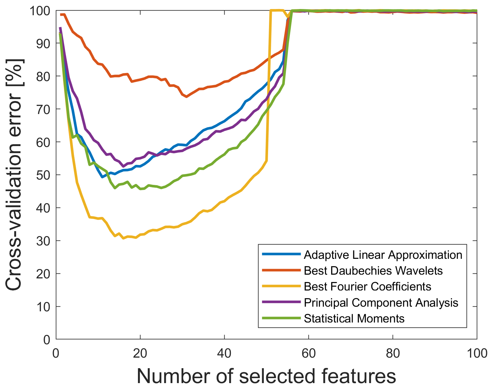
Figure 11 Cross-validation error vs. number of selected features for a maximum time shift of ±50 ms and RFESVM as selector. For a better visibility, only the results with RFESVM as selector are shown.

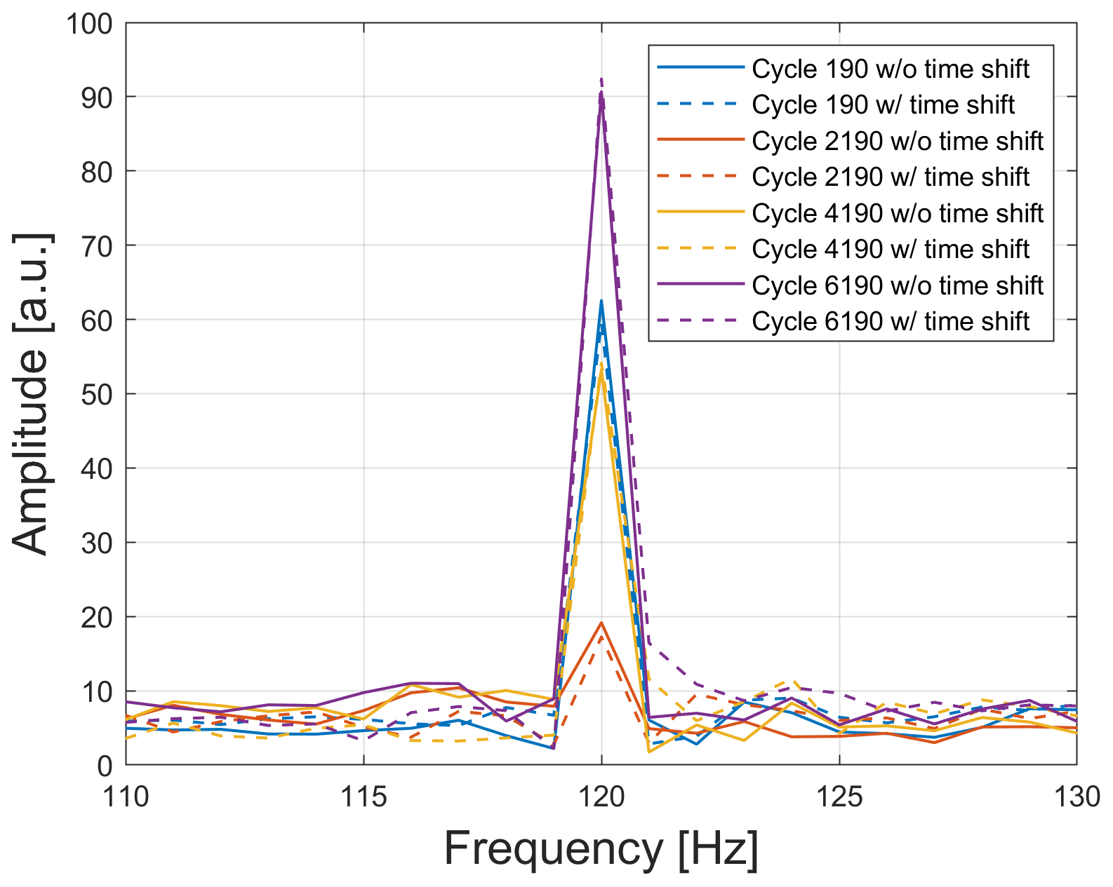
Figure 12 Best feature according to RFESVM (120 Hz of the active current) for the 2 kHz raw data set and the data set with random time shift of maximum 50 ms for three different cycles.

Figure 12 shows the frequency spectra for the 120 Hz feature of the active current (1 of the 17 most relevant features) for different cycles of the raw data set and the data set with random time shift of maximum 50 ms. It can be clearly seen that this amplitude feature changes during the lifetime of the axis, but for different time-shifted data sets, it is nearly the same for the same cycle as for the raw data set. This is shown exemplary here with only one time-shifted data set.

For explanation of this behavior, let x(t) denote the real-valued time domain signal for which information is available at discrete time points t₀, …, t_N−1. The discrete Fourier transform (DFT) for the real-valued sequence X=(X₀, …, $X_{N-\mathrm{1}}{)}^{\top }$ is defined as

$$\begin{array}{}\text{(2)}& {\widehat{\mathit{X}}}_k=\sum _{n=\mathrm{0}}^{N-\mathrm{1}}{\mathit{X}}_n\exp \left(-j{\displaystyle \frac{\mathrm{2}\mathit{\pi }n}{N}}k\right)\mathrm{for}k=\mathrm{0},\mathrm{\dots },N-\mathrm{1}.\end{array}$$

If the DFT of the signal x(t) is given by ${\widehat{\mathit{X}}}_k$, the DFT for the time-shifted signal x(t−s) is given by

$$\begin{array}{}\text{(3)}& {\widehat{\mathit{X}}}_{k,\mathrm{shifted}}={\widehat{\mathit{X}}}_k\exp \left(-j{\displaystyle \frac{\mathrm{2}\mathit{\pi }n}{N}}s\right)\mathrm{for}k=\mathrm{0},\mathrm{\dots },N-\mathrm{1}.\end{array}$$

The spectrum of the time-shifted signal is thus calculated from ${\widehat{\mathit{X}}}_k$, where each spectral component k experiences a frequency-proportional (linear) phase shift of $\exp \left(-j\frac{\mathrm{2}\mathit{\pi }}{N}s\right)$. The amplitude spectrum of the time-shifted signal remains unchanged. Therefore, the amplitudes are robust against time shifts as seen in Fig. 12.

In industrial environments, there are often two different issues when using machine learning. First, there are synchronization problems within a sensor network which can be simulated here by training the model with the raw data set and applying the trained model on the data sets with different random time shifts. Figure 13 shows the classification error using a 10-fold cross-validation, which means the training per fold is carried out with 5663 random cycles of the 2 kHz raw data set; the remaining cycles of different data sets are used for the testing. It can be clearly seen that the classification error increases the larger the time shifts get. The classification error of 17.33 % is reached when applying the model only to the raw test data without time shifts. Applying the model built only with the raw data to time-shifted data with ±0.1 ms already leads to a significant increase of the classification error (48.17 %). Thus, it is crucially important that the different sensors and cycles are synchronized. But when data are not well synchronized or if there is no information about the synchronization, the results can be improved somewhat by excluding the phase features, which can also be seen in Fig. 13. For the data set with ±1 ms time shift, the result can be improved from 95.87 % using the model with amplitudes and the phases to 44.99 % when removing the phases out of the model.

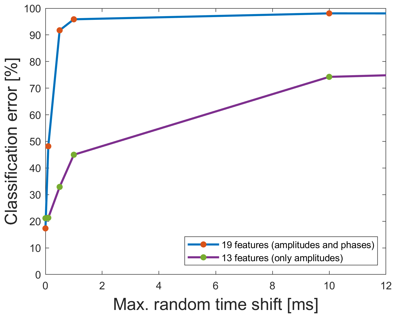
Figure 13 Classification error for one fold of the 10-fold cross validation using the raw data set for the model training and applying this model to data sets with different maximum random time shifts. Red dots represent models based on both amplitude and phase features, while green dots represent models using amplitude data only.

The second important issue is the choice of the time frame. Figure 14 shows that the time frame must be chosen exactly the same for all data sets, because the classification rate for one fold of the 10-fold cross-validation worsens from 17.33 %, applying the raw data for the testing, to 69.63 %, applying the data set with a time frame shifted by only 0.1 ms when using the model trained with the 2 kHz raw data set. In this case, it is also possible to improve the results by removing the phases from the model. For the data with the constant time shift of 0.1 ms, removing the phases and thus using only a model with amplitudes leads to a classification error of 22.26 % instead of 69.63 %.

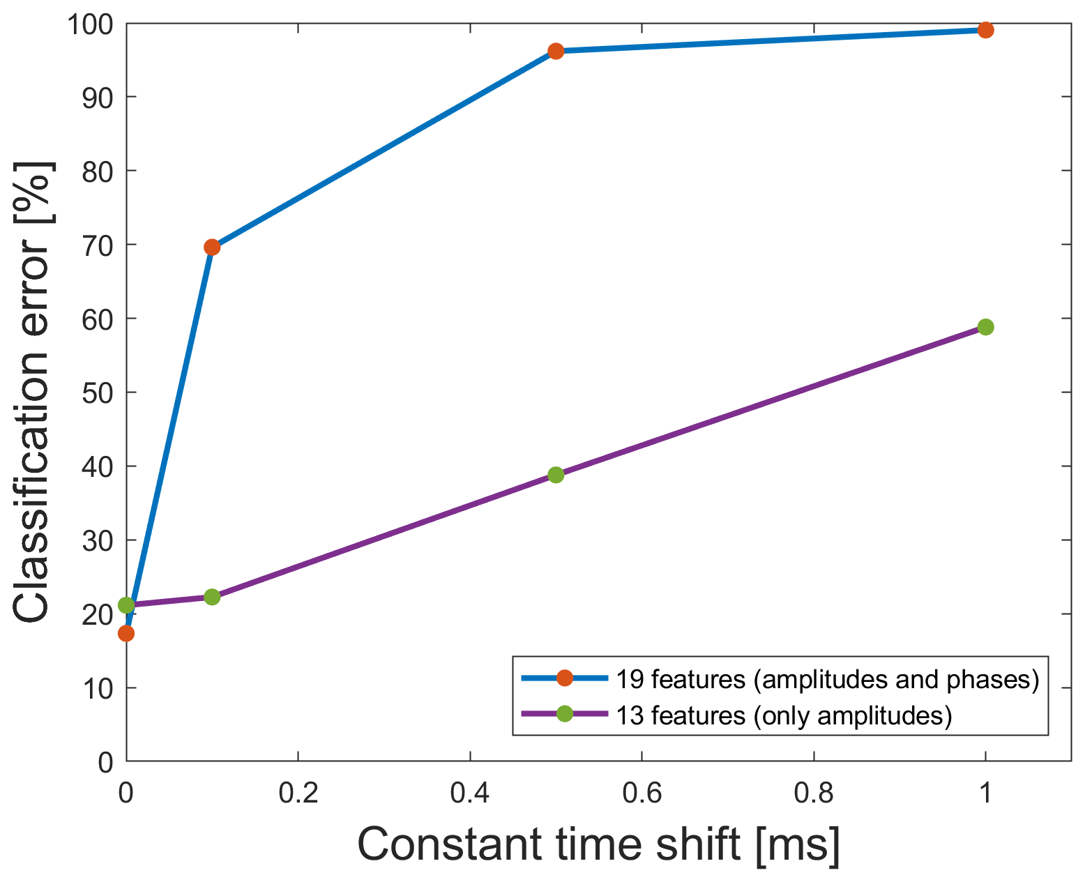
Figure 14 Classification error for one fold of the 10-fold cross validation using the 2 kHz raw data set for the model training and constant time-shifted data sets for the application of the trained model. Red dots represent models based on both amplitude and phase features, while green dots represent models using amplitude data only.

A further improvement of the classification results can be achieved by training the model not only with the raw data but also with synthetically time-shifted data and considering only the amplitude features within the model (cf. Table 4).

Table 4 Classification error for the prediction of the data set with 1 ms time shift by using different models.

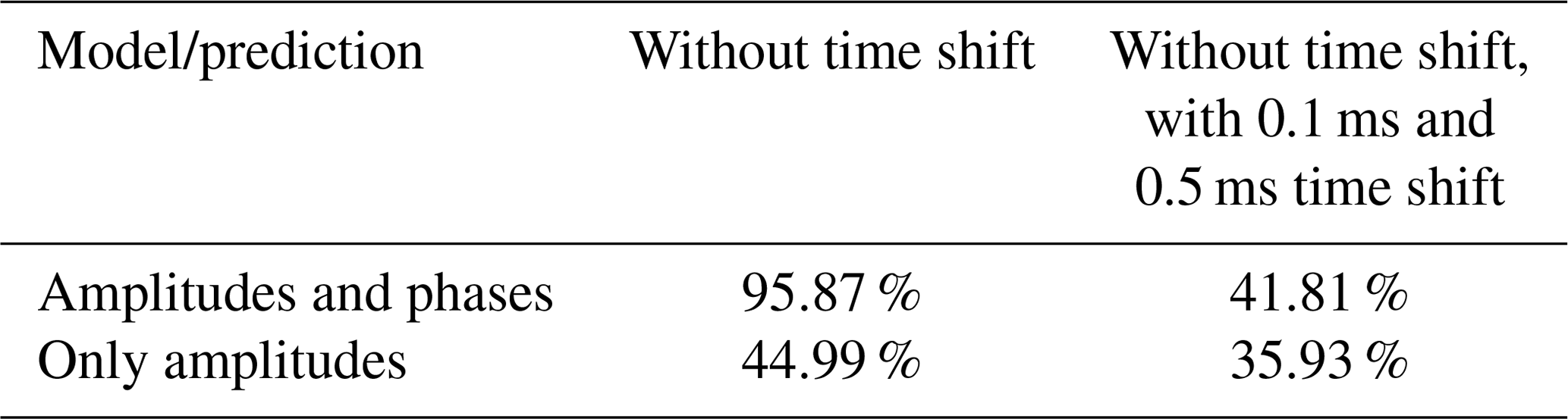
To depict the effect of improving the classification error more clearly, the ±1 ms time-shifted data set is used for the testing of the model in all four cases in Fig. 15. Two different models are considered here. In the upper subfigures, the model was trained only with the 2 kHz raw data set, whereas in the lower ones the ±0.1 and ±0.5 ms time-shifted data are used for the model training in addition. The two subfigures on the left show the prediction of the lifetime with a resolution of 1 % when using the model, as it is resulting from the ML toolbox which means using both amplitudes and phases, whereas in the right ones only amplitudes are used. It can be clearly seen that the best classification error of 35.93 % for the ±1 ms time-shifted data set is reached with the model which is additionally trained with time shifts and consists of only amplitudes.

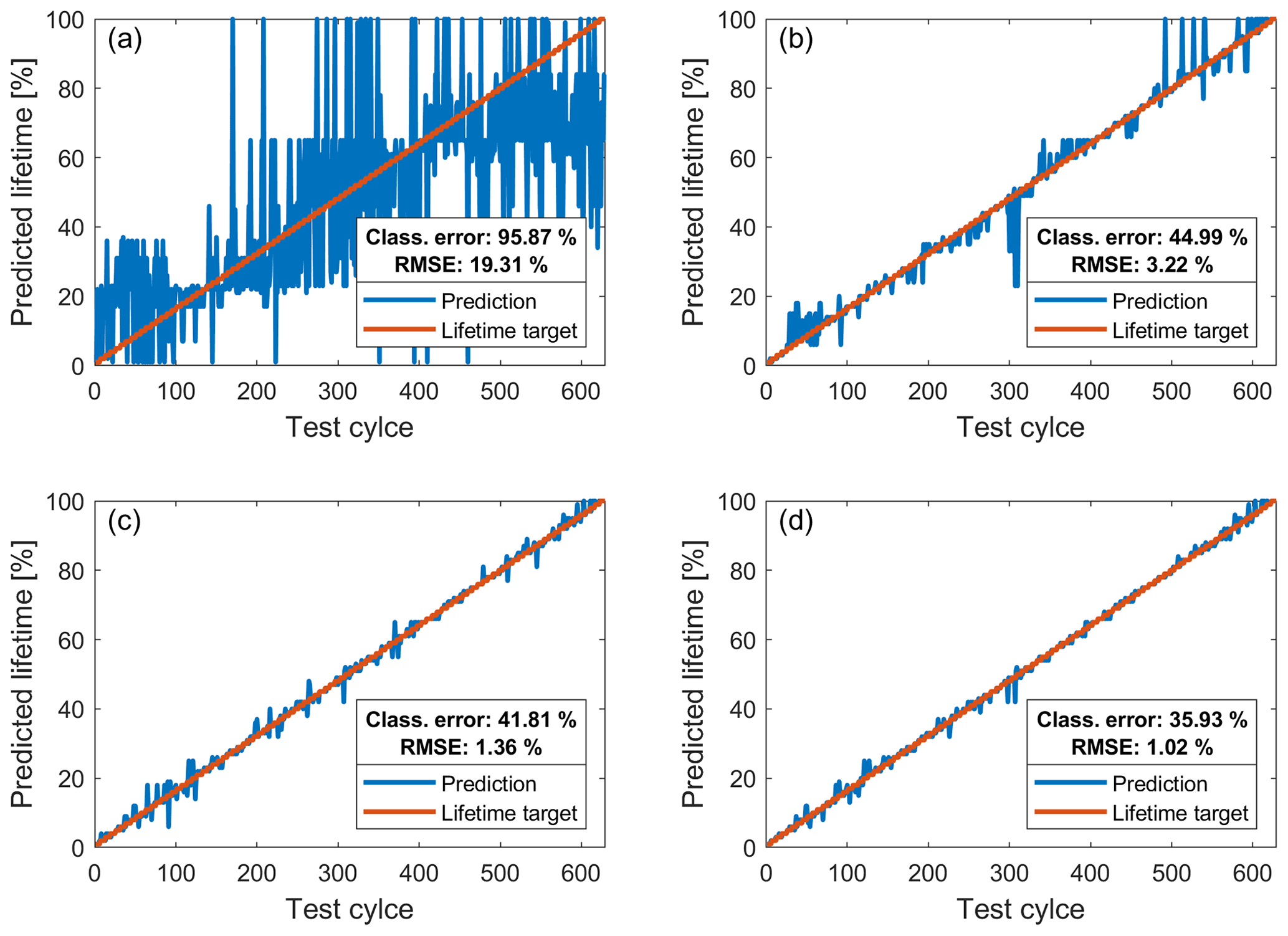
Figure 15 Predictions (blue) of the used EMC lifetime (steps of 1 %) for one fold of the 10-fold cross validation for the data set with time shifts of up to 1 ms and the assumed used lifetime target from 1 % to 100 % (red). (a) Model trained with raw data only using both amplitude and phase features. (b) Model trained with raw data only using only amplitude features. (c) Model trained with raw, 0.1, and 0.5 ms time-shifted data sets using both amplitude and phase features. (d) Model trained with raw, 0.1 and 0.5 ms time-shifted data sets only using amplitude features.

6 Conclusion and outlook

In this contribution, data sets with time synchronization errors were considered to investigate their influence on results obtained with a ML software toolbox for condition monitoring and fault diagnosis. Minimal synchronization errors between the individual sensors, when already present in the training data, only have a small effect on the cross-validation error achieved with the ML toolbox. However, if ML models are trained without any synchronization errors, applying these models to data sets even with minimal time shifts of 0.1 ms results in large classification errors, here for the prediction of the RUL of a critical component. This error can be reduced by modifying the feature extraction and excluding phase values after Fourier analysis in a first step. By adding artificially time-shifted data to the training set, a further improvement of the classification result is achieved. Thus, the study presented in this contribution provides important guidelines for improving the setup of distributed measurement systems, especially about the necessary synchronization between sensors. If no information about the synchronization within the network is available, it is suggested to generate artificially time-shifted data sets from the original data and use this extended data set for training the ML model. Note that this is similar to data augmentation suggested for improving the performance and robustness of neural networks (Wong et al., 2016).

It is also important to choose the time frame for the 1 s period correctly. Applying the model to data even with only a small shift of 0.1 ms of the time frame in comparison to the training data already leads to very poor classification results.

For future work, measurement uncertainty should be considered in addition to time synchronization errors as both contribute to data quality and are therefore expected to have a strong influence on ML results for condition monitoring or fault diagnosis. In the European research project “Metrology for the Factory of the Future” (Met4FoF), mathematical models for the consideration of metrological information in ML models are developed. For example, the project considers the classification within the ML toolbox by reviewing the robustness of the LDA as a classifier when using redundant features. Specifically, we will study how long the quality of the LDA results continues to improve with additional features and when the point is reached where the LDA fails, because the covariance matrix becomes singular; i.e., its determinant disappears.

The current ML toolbox (see Fig. 3) does not take any measurement uncertainties into account. To overcome this limitation, the methods included in the toolbox are extended to allow for more robust and accurate failure analysis or condition monitoring applications such as predicting the RUL of components as discussed in this paper. The uncertainty evaluation for the BFC method was already presented by Eichstädt and Wilkens (2016). The uncertainty evaluation for ALA was recently published (Dorst et al., 2020). The uncertainty evaluation for the remaining three feature extraction methods is already developed and will be published soon. Thus, the ML toolbox can then provide features together with their uncertainty as determined from the uncertainty of the raw sensor data. Furthermore, the three feature selection algorithms can be replaced by filter-based selection algorithms which weight the features based on their uncertainties. Finally, the propagation of the uncertainty values through the LDA classifier is also completed. Thus, the extended ML toolbox, soon to be published, will be able to take the uncertainty of measured data into account to achieve improved models. In the future, we plan to add wrapper and embedded methods for the feature selection step of the ML toolbox that also consider uncertainties.