the Creative Commons Attribution 4.0 License.
the Creative Commons Attribution 4.0 License.
 | 13 Oct 2021
Characterization of specular freeform surfaces from reflected ray directions using experimental ray tracing
Tobias Binkele
David Hilbig
Mahmoud Essameldin
Thomas Henning
Friedrich Fleischmann
Walter Lang
The applications of freeform surfaces in optical components and systems are increasing more and more. Therefore, appropriate measurement techniques are needed to measure these freeform surfaces for verification. This task is still a challenge for most measurement techniques. In this paper, we propose a measurement technique for optical and other specular freeform surfaces based on experimental ray tracing. This technique is able to measure form and mid-spatial-frequency deviations simultaneously. The focus will be set on the sensing technique and the measurement uncertainties in the setup. As the measurement technique is described, an estimation of the influence of different uncertainties based on simulations is given. The result from an experimental measurement is evaluated in relation to the influence of the uncertainties. A comparison measurement for evaluation is given.
- Article
(4861 KB) - Full-text XML
- BibTeX
- EndNote


Freeform surfaces are the next level in the evolution of optical surfaces. After spherical and aspherical surfaces, they open new degrees of freedom to design optical components (Thompson and Rolland, 2012). However, the quality of the manufactured surfaces has to be verified to ensure the desired functionality in the optical system. We target this need for verification using a variation of the measurement technique called experimental ray tracing (ERT) (Häusler and Schneider, 1988). Originally, ERT was introduced as a modification of the Hartmann test with modern hardware (Hartmann, 1904). The target was to measure the function of optical components and systems in transmission. A measurement system based on this original proposition has been implemented (Ceyhan et al., 2011). Besides this implementation, the measurement technique has also proven its enormous abilities in different variations and data analysis methods. This includes the precise measurement of the paraxial focal length of optical components (Binkele et al., 2016), the performance measurement of progressive addition lenses (Gutierrez et al., 2017a), the characterization of secondary optics for LEDs (Gutierrez et al., 2017b) and even the refractive index measurement in gradient-index lenses (Binkele et al., 2019a). The original measurement system implemented by Ceyhan et al. (2011) was already able to determine surface imperfections in the range of form and mid-spatial-frequency of spherical and aspherical lenses. These imperfections are derived from the determined optical function. This means that the optical component was investigated for its ability for the accurate refraction of incoming rays. If the refracted ray direction deviates from the expected direction, a surface imperfection can be estimated from the magnitude of the deviation. As this technique measures in transmission, the mapping of the imperfections to one of the surfaces was only possible by assuming the other surface being error-free. Having one surface being much more prone to imperfections due to the manufacturing process, the assumption was justified and the determined surface imperfections were comparable to results from other measurement techniques. However, the theoretical ambiguity in the mapping of the surface error cannot be overcome with this technique. This issue does not exist for surfaces tested in reflection. Additionally, even specular surfaces of non-transparent objects, like drive shafts, can be measured. Thus, we modified the principle of ERT in a way not to measure the surface under test (SUT) in transmission, but in reflection. This opens the possibility of using the abilities of the sensing technique while overcoming the ambiguity in the measurement results.
ERT is based on the measurement of a deflected ray's direction. In the original proposition of ERT, this deflection is introduced by refraction (Häusler and Schneider, 1988). In contrast to that, in the measurement setup proposed here, the deflection is introduced by reflection. Therefore, the setup has to be adapted. The proposed measurement setup is shown in Fig. 1.
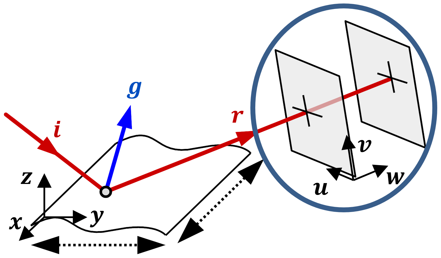
Figure 1Sketch of the proposed measurement setup and the ray direction sensing component. The two coordinate systems shown represent the orientation of the SUT (x, y, z) and ray direction sensing component (u, v, w).
The incident ray is directed onto the SUT having a certain direction i. After being reflected, the direction of the ray is changed. The reflected ray's direction r depends on i and the direction of the surface normal g at the point of reflection. Thus, having the directions i and r as unit vectors, the surface normal
can be calculated using vector geometry (Mikš and Novák, 2012). To collect information about a certain area, the SUT is moved linearly along the dashed lines shown in Fig. 1. Thereby, the desired area is scanned at discrete positions. Unfortunately, the actual points of reflection can deviate from the discrete points set for the scanning. This deviation is dependent on the incident ray direction i and the shape of the SUT. This problem is overcome for known surfaces by considering the expected known model for the evaluation. For unknown surfaces, the field of view can be changed in a way that the deviations are irrelevant (Binkele et al., 2019b). Having the actual points of reflection determined, a Cartesian coordinate system with the axis x, y and z is introduced to transfer the detected surface normal into the surface slopes:
where p represents the slope in x direction and q represents the slope in y direction. Although one could expect an approximation in Eq. (2), these equations are exact as slopes are calculated and not angles. This gets more clear regarding Fig. 2, where the vector components for the calculation of p in Eq. (2) are illustrated.

Figure 2Illustration of the relation between the normal vector components gx and gz and the surface slope p calculated using Eq. (2).
A 2D-integration method based on radial basis functions is used to reconstruct the surface (Ettl et al., 2008). As this is a global integration method, errors are distributed over all sample points and propagation of errors is suppressed. However, if noisy data are faced, the integration parameters can be adapted to make the integration method more robust (Lowitzsch et al., 2005).
For the determination of the surface normal directions, the incident ray direction i and the reflected ray direction r have to be known. The detection of the direction of the reflected ray is performed using a ray direction sensor. The circle in Fig. 1 marks the position of the sensor in the setup. The basic idea of the ray direction sensor is the detection of two different positions of the ray in space. Therefore, a flat sensor that detects the ray location R on its surface is used. Moving this sensor in a known direction and distance, a second point S is detected. From these two known points that the ray intersects with, the reflected ray direction
can be determined. A sketch of the sensor principle is shown in Fig. 3.
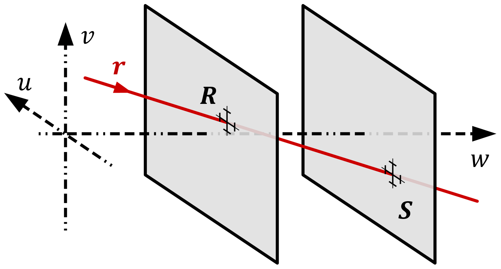
The implementation of this principle in a real measurement setup can be realized in different ways. In our setup, we represent the incident ray by a narrow laser beam. The width of the beam is approximately 300 µm. For the beam position detection, we use a bare camera chip in combination with a centroid detection algorithm (Hu, 1962). To measure the two points R and S, the camera is mounted on a linear stage, assuring the positioning in a known direction and distance. The positioning of the SUT is also realized using linear stages.
3.1 Uncertainty determination principle
To determine the uncertainties of the measurement technique, we have simulated different uncertainty sources independently. In this way, the influence of each source can be detected separately. The considered sources are each described and analyzed in the following subchapters. Finally, all sources are combined together in one simulation to get an overall uncertainty estimation for the investigated sources. To have a good comparability to the measurement results given later, the same SUT model and measurement parameters are used in the simulations as are later used in the experimental measurements. This also includes the 2D-integration process. The value compared is the root-mean-square (rms) surface deviation between the expected surface and the reconstructed surface. The SUT used is a polynomial freeform. The surface follows the function
Its surface topography is shown in Fig. 4.
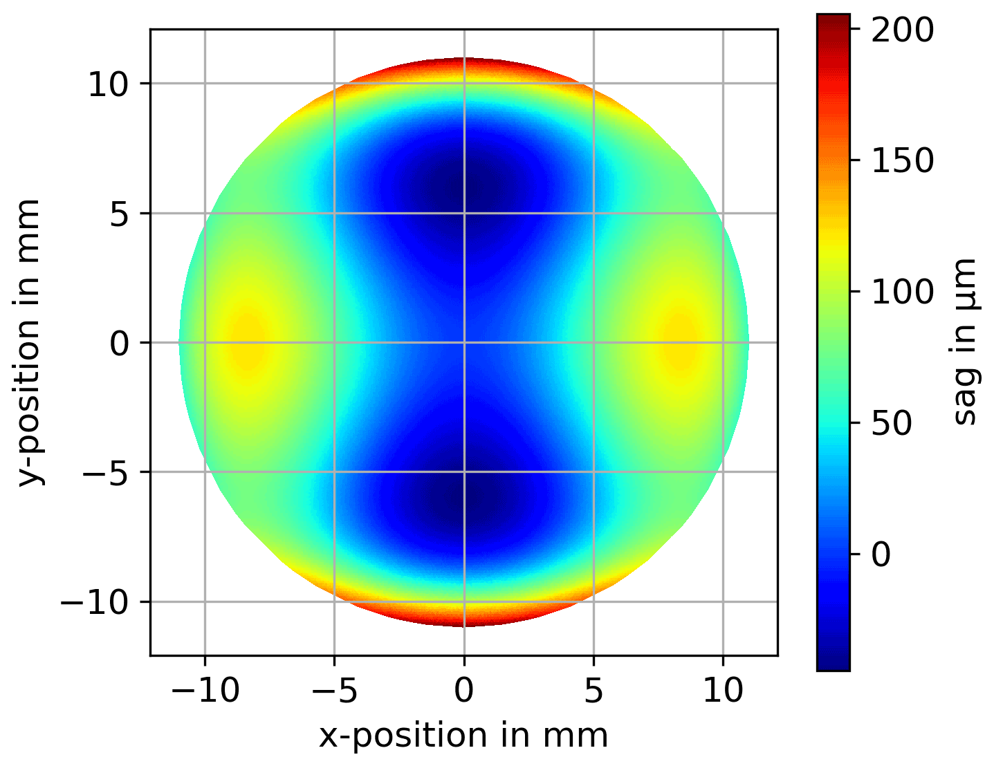
The considered area of the SUT is circular with a diameter of 22 mm. The sample points are arranged in a Cartesian grid with a spacing of 100 µm. In the considered area, the SUT has a peak to valley (PV) of approx. 350 µm and a maximum surface angle of approx. 8.5∘. The simulations have been performed using Zemax OpticStudio (Zemax LLC, 2020). For the data evaluation, the Python distribution Anaconda is used (Anaconda, 2020). Anaconda is an open collection including many often-used packages while maintaining compatibility between the package versions.
3.2 Centroid determination
The measurement setup is built up in a dark box. Multiple noise sources influence the determined position of the centroid on the camera chip. This includes dark current, shot noise and also centroid instability of the incident beam (EMVA Standard 1288, 2016; Levesque et al., 1996). These sources sum up to a compound uncertainty of the centroid determination. The uncertainty bars at R and S in Fig. 3 visualize this uncertainty.
To determine the uncertainty of the centroid detection experimentally, a flat mirror is placed in the setup. This leads to a reflection of the incident beam into the camera. Without moving the mirror or any other object in the experimental setup, the centroid position is observed. To get an appropriate amount of data, 1000 images are taken and evaluated over 4 min. The measured centroid data in u and v direction are shown in Fig. 5.
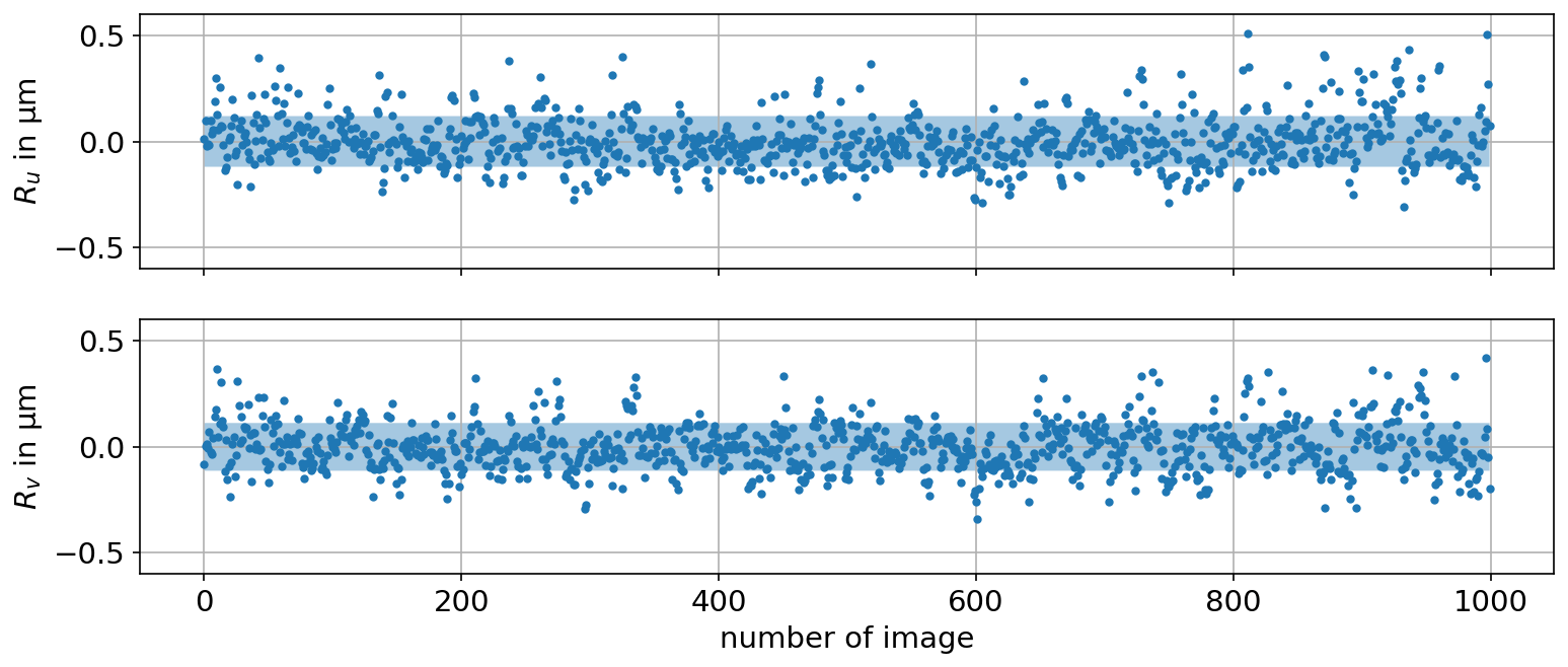
Figure 5Detected centroid positions over 1000 images for one detection plane. The blue area visualizes the detected standard deviation in both directions (σu=120 nm, σv=113 nm).
To observe the statistical error only, a slight linear drift, determined by linear regression, has been subtracted from the data. The drift has been detected to be 66 nm in u direction and 2 nm in v direction over the 1000 images and is caused by thermal expansions in the setup. Different components used for the mounting of the camera and the SUT lead to the large difference of the drift in the two different directions. The warm-up time until stabilization is 1 h. The blue area visualizes the span of the detected standard deviation σu=120 nm and σv=113 nm in both directions. Regarding the camera's pixel size of 7.4 µm by 7.4 µm, this corresponds to a centroid detection uncertainty of px in u and px in v direction.
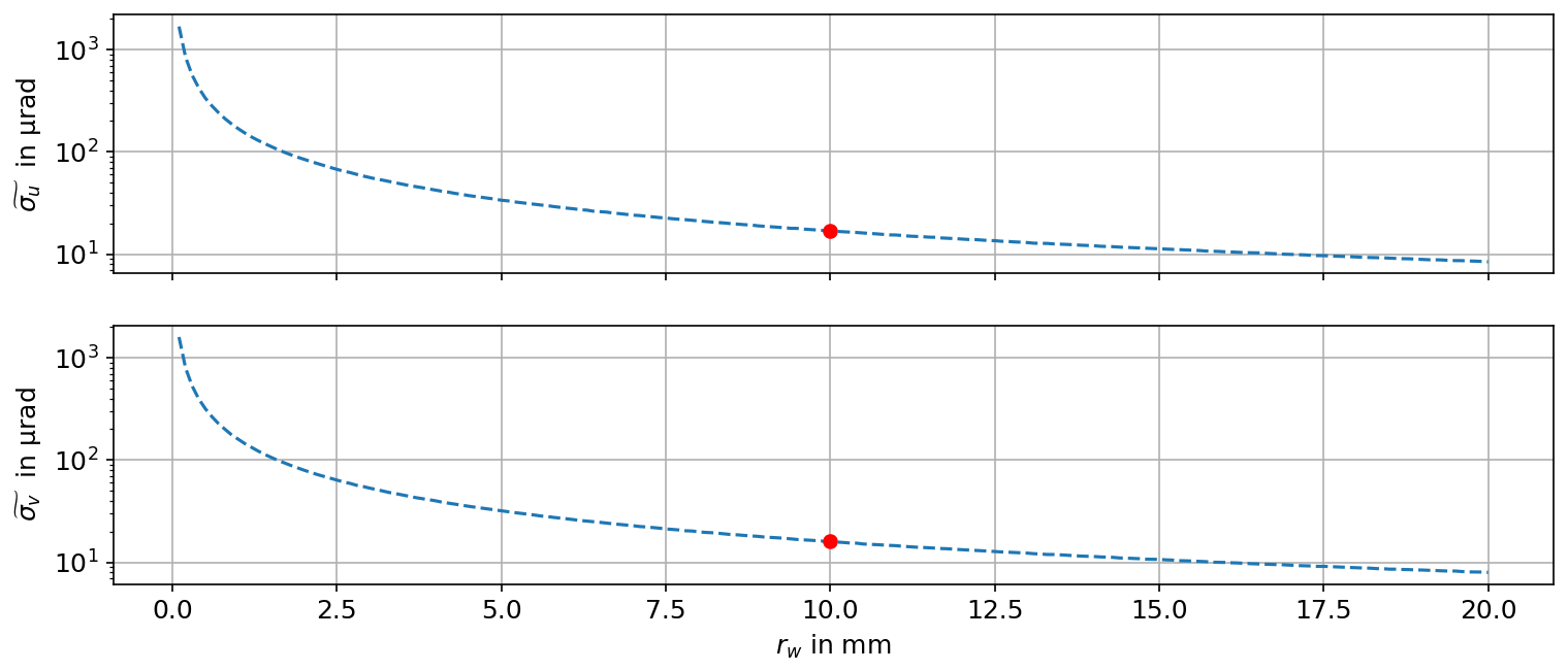
Figure 6Determined ray direction uncertainty over the distance rw between the two detection planes. The markers indicate the values considered for the further estimation of the influence on the results of the measurement setup.
To transfer these centroid detection uncertainties to the uncertainties of the ray direction and in u and v direction, one more piece of information is needed and evaluated: the distance between the two detection planes. Here, the ray direction is defined as the ray's angle to the w axis in u and v direction
where represents the distance between the two detection planes. From Eq. (5), one can see that the influence of the centroid detection uncertainty on the ray detection uncertainty decreases with an increase of rw. To evaluate the actual values of and dependent on rw, a Monte Carlo simulation has been performed (Lira, 2002). In this simulation the value of rw has been changed from 0.1 to 20 mm in steps of 100 µm. For each value of rw, 100 000 simulations of a ray direction detection including the uncertainties σu and σv have been performed. Applying the data to Eq. (5), the values of and can be evaluated for each value of rw. The results from the simulation are shown in Fig. 6.
For further considerations, the distance rw is set to 10 mm. This leads to a ray direction uncertainty of µrad and µrad.
A simulation of the measurement of the SUT, as described in Sect. 3.1, has been performed. To determine the influence of the stochastic centroid determination uncertainty, this simulation has been performed as a Monte Carlo simulation. The results show a mean value for the rms surface deviation over the simulation iterations of 1.7 nm.
3.3 Camera positioning and orientation
The positioning of the camera is performed using a linear stage that moves the camera along the w axis to determine the reflected rays direction r in two different planes, as shown in Fig. 3. This linear stage has a feedback system with a resolution of 100 nm and, according to the manufacturer's test protocol, a positioning uncertainty of ±600 nm PV. To evaluate the maximum influence on the results, the simulation is performed having the maximum positive deviation for the first camera position and the maximum negative deviation for the second camera position. This leads to an rms surface deviation for the simulated measurement of 6.4 nm due to the camera positioning uncertainty.
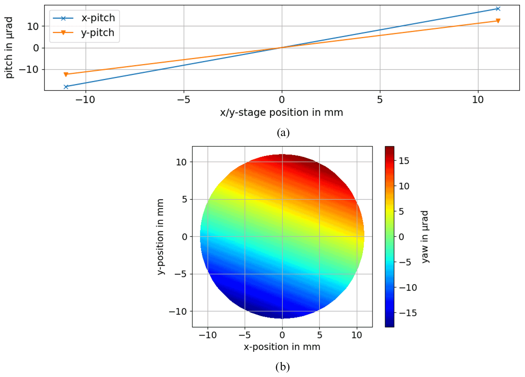
Figure 7(a) Evolution of the assumed pitch for the x and y stages for the simulation. (b) Evolution of the yaw, rotation around the z axis, dependent on the sample point position.
The positioning stage for the camera also includes an uncertainty in terms of pitch, represented by a rotation around v axis, and yaw, represented by a rotation around the u axis, of the camera stage. According to the manufacturing's test protocol, the pitch has a PV of ±18 µrad and the yaw has a PV of ±13 µrad. Equivalent to the determination of the influence of the camera positioning, the influence of the pitch and yaw has been investigated by having the maximum positive pitch and yaw on the first camera position and the maximum negative pitch and yaw on the second camera position. This leads to an rms surface deviation for the simulated measurement of 0.4 nm due to the camera pitch and yaw.
3.4 SUT positioning and orientation
Similar to the positioning and the pitch and yaw of the camera, the same types of uncertainties apply to the positioning and orientation of the SUT. First, the positioning in x and y direction is considered. The manufacturer's given uncertainty is also ±600 nm PV. However, as the SUT is positioned to 37 977 different sample points over the circular aperture within the simulation process and the distribution is not known, this uncertainty is considered stochastic and triangular-distributed. Using the triangular distribution considers the information that a given targeted value exists as well as the information of the given PV boundaries. Evaluating the influence of this uncertainty, using a Monte Carlo simulation, leads to an rms surface deviation of 0.5 nm. It has to be pointed out that this is only valid for the given surface model, as this value is dependent on the surface function. If the model was flat, the positioning uncertainty of the SUT had no influence on the determined surface slope.
According to the manufacturer's test protocol, the x stage has a PV pitch of ±18 µrad and a PV yaw of ±6 µrad. Regarding the y stage, a PV pitch of ±12 µrad and a PV yaw of ±17 µrad has been protocolled. For the simulation of the influence of these values, a linear evolution of the pitch and yaw for each stage from the most negative to the most positive position within the considered area is assumed, while the yaw from both stages is added. The evolution of the pitch of each stage and the combined yaw is illustrated in Fig. 7.
The simulation using these values for the pitch and yaw leads to an rms surface deviation of 6.4 nm.
3.5 Incident beam direction determination
For the determination of the incident beam direction, different ways have already been approached (Binkele et al., 2017; Hilbig et al., 2017). Although these techniques are applicable without knowing the SUT model for reference, they have been observed not to be accurate enough for a satisfying result. Thus, we have chosen to use a new technique for the determination of the incident beam direction. This technique is only applicable if the expected surface model is known. It is based on the minimization of the deviation between the reconstructed and the expected surface while optimizing the incident beam direction. Therefore, one measurement result from the SUT is evaluated with an initial guess of the incident beam direction. In the simulation, the incident beam direction is now varied to evaluate the deviation between the reconstructed and the expected surface for different incident beam directions. Finding the incident beam direction, where this deviation is minimized, the incident beam direction is found. To determine the uncertainty of this technique we have performed a Monte Carlo simulation applying the centroid determination uncertainties σu and σv to the simulation described in Sect. 3.1. This leads to a standard deviation of the incident beam determination of 6 µrad. Using this standard deviation value for a Monte Carlo simulation, an rms surface deviation of 0.6 nm has been determined.
3.6 Summary of uncertainty determination
To determine the combined influence of all error sources, one has to regard that the model is non-linear. Thus, a Monte Carlo simulation has been performed (JCGM, 2008). Equivalent to the positioning of the SUT, the positioning of the camera has also been assumed to be triangular-distributed with a PV of ±600 nm. From this simulation, a mean rms surface deviation of 25.2 nm is determined. The simulation was performed until the mean rms value did not change more that 0.01 nm over the last 10 iterations. Therefore overall 253 iterations were performed. Table 1 gives an overview of all determined results from the previous chapters including the result considering all sources combined.
Although Table 1 already shows the influence of six sources of uncertainties, the list does not claim to be complete. For example, an uncertainty that has not been considered here is the roll of the camera positioning stage, as there is no information given for this value from the manufacturer. Another example can also be irregularities in the camera chip or a non-ideally orthogonal orientation of the x and y stage. It has to be mentioned that the straightness and flatness of the camera stage and the xy stages have not been considered here. Additionally, influences by change of the environmental conditions in the measurement room, e.g., centroid drift introduced by temperature variations, have not been taken into account. On the other hand, it has to be mentioned that for the camera orientation and the SUT orientation, the given PV values for the full travel length of these stages are used. The full travel length of these stages is 100 mm, but the camera positioning only needs 10 mm distance and the SUT positioning only 22 mm distance. Although this cannot be said for sure, it is expected that the uncertainties are smaller than they have been considered here for the simulations.
Table 1All considered uncertainties and their individual and combined influence on the rms surface deviation from the simulation of the measurement of the polynomial freeform described in Sect. 3.1.
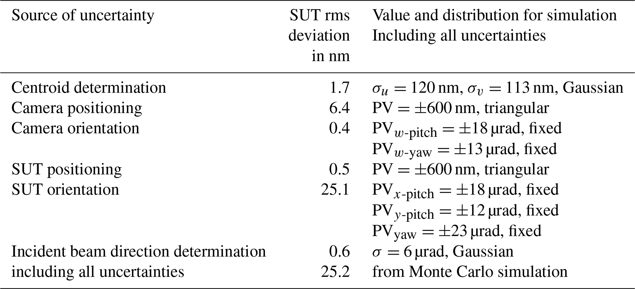
In Table 1 one can clearly recognize that the SUT rms deviation in the Monte Carlo simulation, including all considered error sources, is dominated by the SUT orientation error. Thus, a solution to determine the systematic errors in this error source has to be found.
To perform experimental measurements, the sketch shown in Fig. 1 has been built up in a real setup. The incident beam has been realized using a fiber-coupled laser diode with a wavelength of 633 nm and an output power of approx. 2 mW. To create a narrow laser beam, the light is coupled out of the fiber through a fiber collimator. The positioning of the SUT is performed by a xy linear stage system. The stages have a maximum travel of 100 mm and a feedback system with a resolution of 100 nm. As described in Sect. 2, a bare CCD camera chip with a size of 24 mm (u direction) by 36 mm (v direction) is used as the beam positioning detector. The total number of pixels is 3232 (u) by 4864 (v) pixels with a square pixel size of 7.4 µm by 7.4 µm. An image from the camera chip with the spot is shown in Fig. 8. The elliptical shape of the spot shown in the magnified image is created by the different curvatures of the surface in x and y direction.
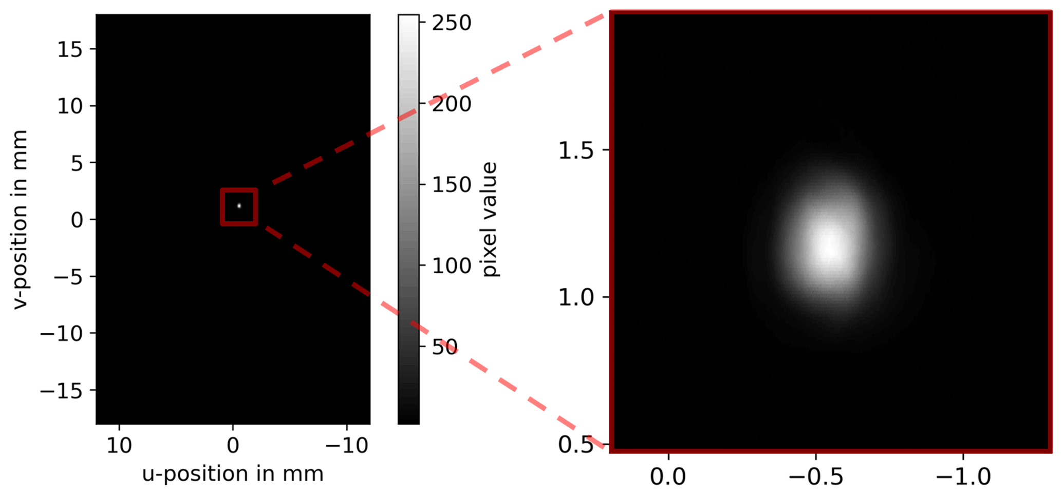
Figure 8Image from the camera showing the spot at an arbitrary position of reflection on the camera chip.
For the positioning of the camera within the ray direction sensor, a linear stage, different from the ones used for the xy positioning, with a maximum travel of 100 mm and a feedback resolution of 100 nm is used. To maximize the range of surface angles that can be measured, the first camera position is as close as possible to the SUT. As described in Sect. 3.2 the distance between the camera planes is set to 10 mm. Surface angles can be measured if the deflected beam still hits the camera chip at the second camera position. If smaller surface angles are expected, the distance between the camera positions can be increased, resulting in a decrease of the ray direction uncertainty as shown in Fig. 6.
To suppress reflections from the second surface, the sample with the SUT is placed on a piece of dark glass from welding goggles. Index-matching liquid is used to fill the gap between the surfaces of the sample and the dark glass. Thereby, the light being refracted into the substrate of the sample is transferred into and absorbed by the dark glass. An image of the setup including the SUT and the dark glass is shown in Fig. 9.
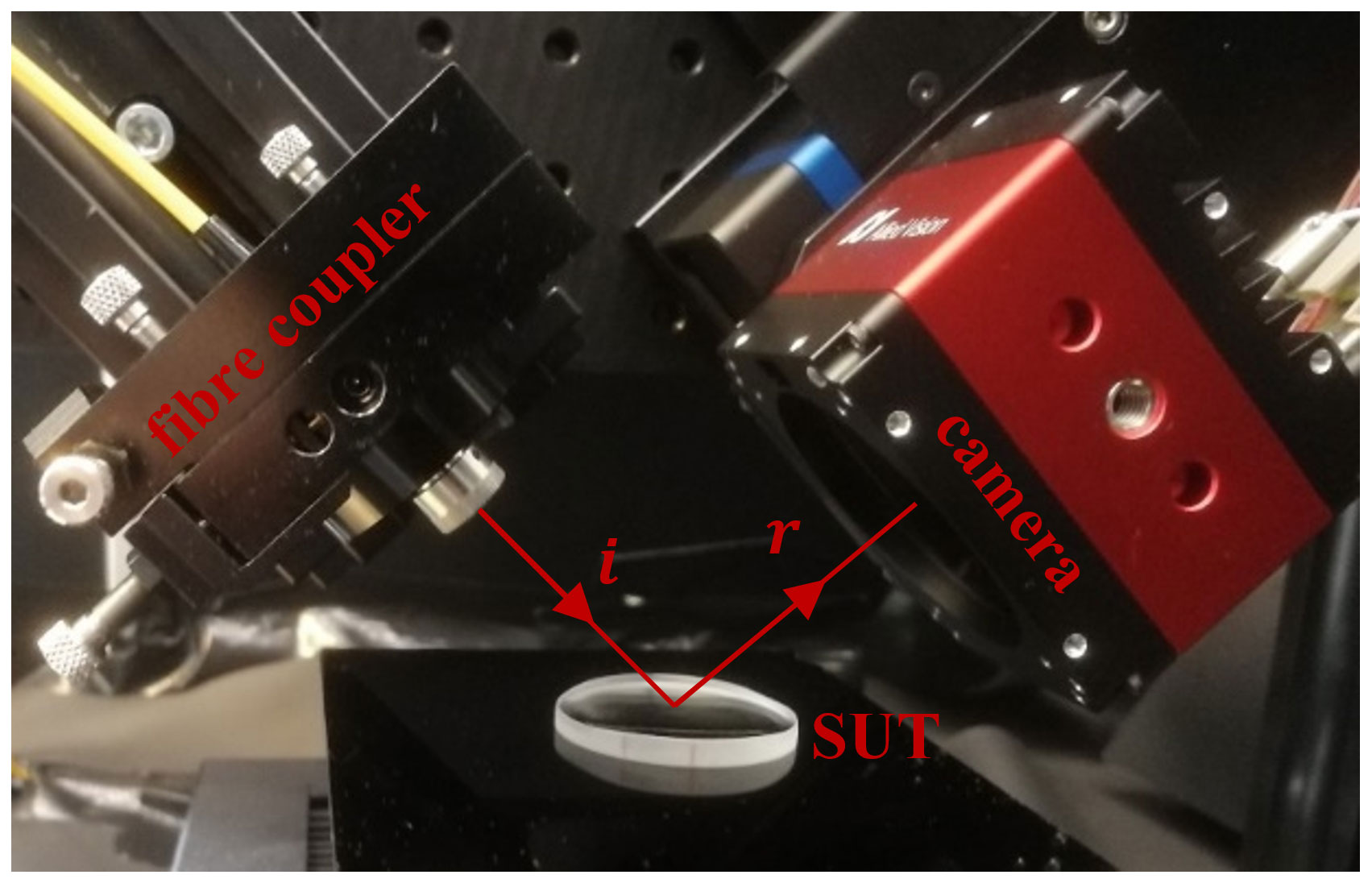
Figure 9Image of the experimental setup with the fiber coupler including the collimator, the incident beam direction i, the SUT, the reflected beam direction r and the camera with the bare chip.
As described in Sect. 3.1, the SUT is a polynomial freeform following Eq. (4). It was manufactured by Trionplas GmbH, Leipzig, Germany, using atmospheric plasma jet machining (Arnold et al., 2014; Paetzelt et al., 2015). An image of the sample is shown in Fig. 10.
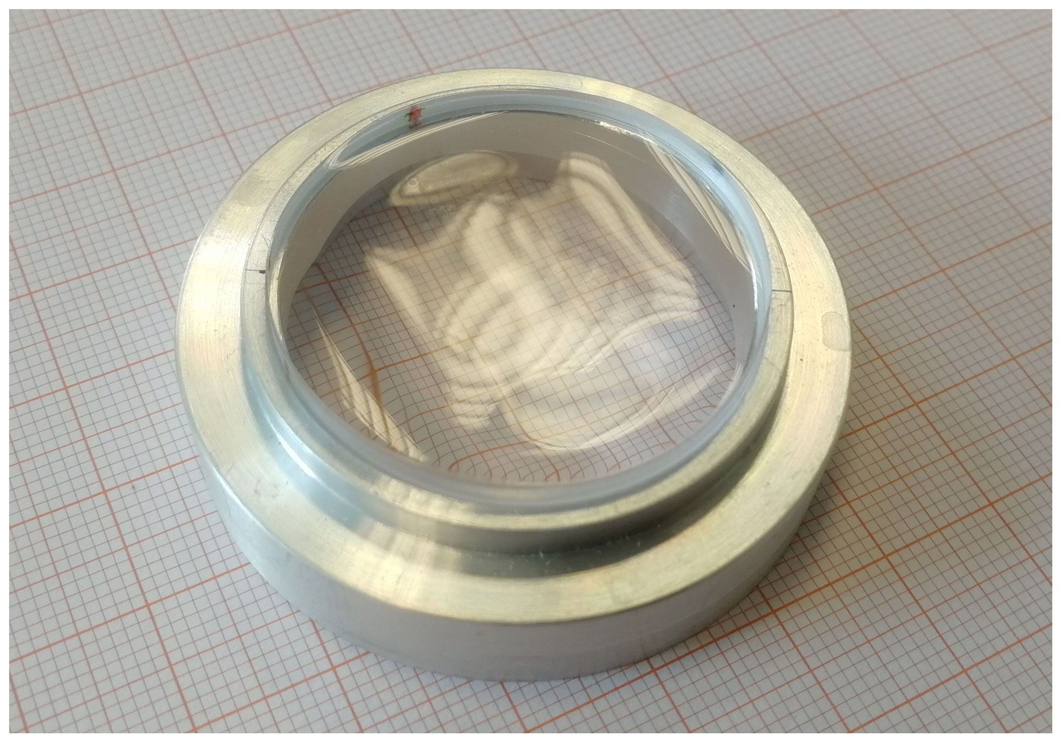
Figure 10Image of polynomial freeform SUT manufactured using atmospheric plasma jet machining.
For better alignment and comparison, three fiducials have been manufactured into the surface. They are all located at a distance of 11 mm from the center, and the second and third fiducial positions are rotated by −30 and −90∘ from the first position. The three fiducials are marked and can clearly be seen in the results from the experimental measurement shown in Fig. 11c. The measurements have been performed using the same measurement parameters as described in Sect. 3.1 for the simulations.
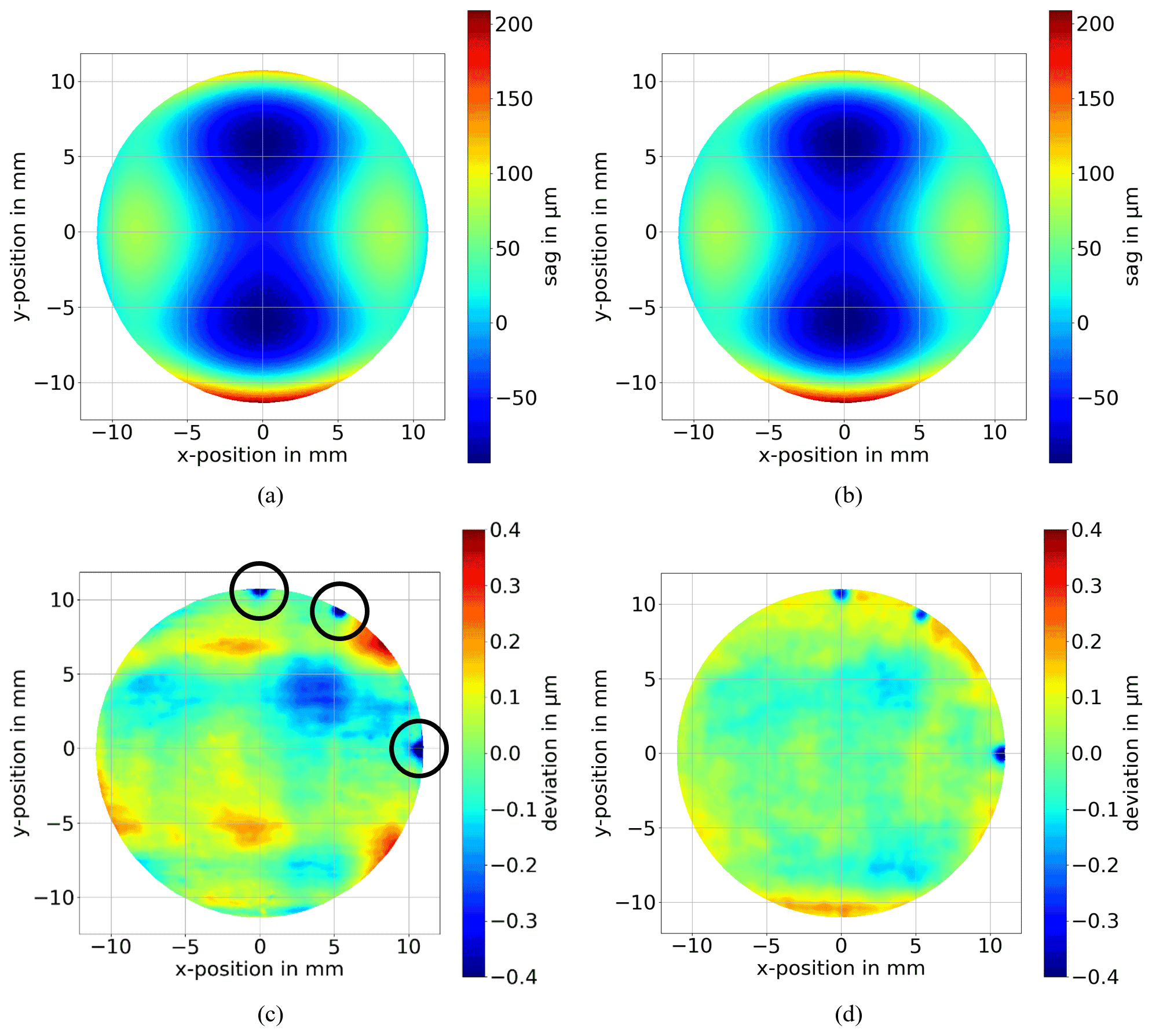
Figure 11Results of the experimental measurement of the polynomial freeform. Panel (a) shows the reconstructed surface. Panel (b) shows the expected model. Panel (c) shows the deviation from the expected model of the SUT. The rms surface deviation is 94 nm. The circles indicate fiducials implemented for better orientation. Panel (d) shows the comparison measurement from the manufacturer performed using a CT 300 by cyberTECHNOLOGIES GmbH. This comparison measurement has an rms surface deviation of 63 nm.
Figure 11a shows the reconstructed surface, which has an rms of 51.476 µm. To get the deviation, the model, shown in Fig. 11b, has been fitted to the reconstructed surface. The deviation determined between the reconstructed surface and the fitted model is shown in Fig. 11c. It has a PV of approx. 1.206 µm and an rms of approx. 94 nm.
Regarding the rms value of the reconstructed SUT and the rms value determined for the uncertainties from the simulations, a factor of can be determined. However, one has to consider that this factor is dependent on the investigated SUT.
To set the measurement in relation, a comparison measurement is used. This measurement has been performed by the manufacturer of the SUT using a CT 300 by cyberTECHNOLOGIES GmbH. The CT 300 is a non-contact profilometer with a white-light distance sensor to measure the surface sag. Its single-point accuracy is ±150 nm PV over the considered area. The determined deviation of the measurement from the design shape is shown in Fig. 11d. The rms surface deviation is 63 nm. Comparing the two measured deviations shown in Fig. 11c and d, one can clearly see that they do not match exactly. In the deviations detected from the technique proposed in this paper, peaks can been seen at the upper right and lower right edge. Furthermore, the overall magnitude of the deviations is higher than the magnitude of the deviations detected by the comparison measurement. This explains the deviation in the rms values of the two measurements. However, one can also observe similar structures, like the two major dips in the upper right and lower right area next to the center. These dips have been detected by both techniques at the same position on the surface.
The differences between the two measurement results shown in Fig. 11c and d are presented in Fig. 12.
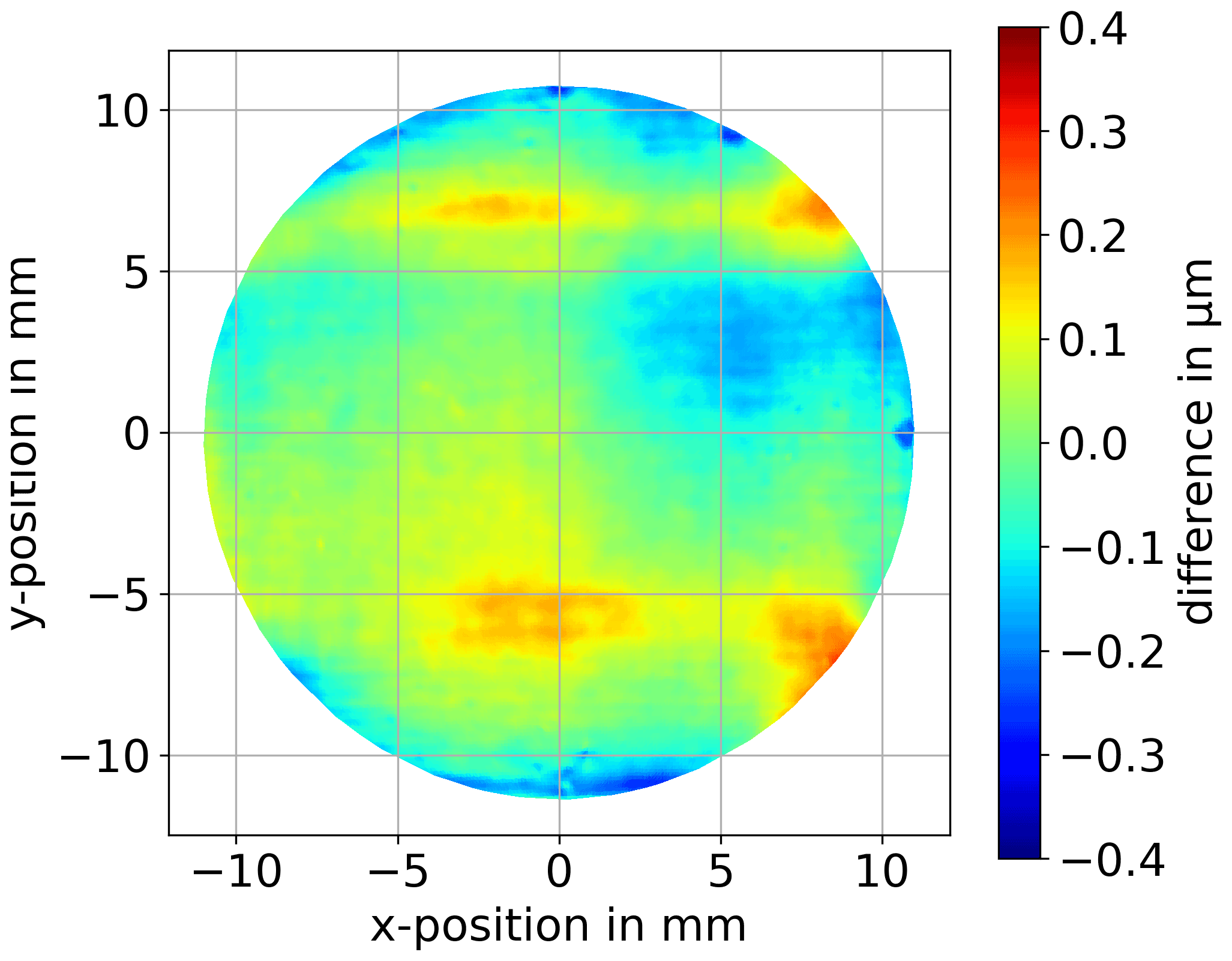
Figure 12Difference between the two determined deviations from the model with the proposed method (shown in Fig. 11c) and the CT 300 (shown in Fig. 11d).
In this paper, we proposed a measurement technique for freeform surfaces. The principle is based on the scanning of the surface with a narrow laser beam and a beam direction sensor after the reflection. The basic idea of the direction sensor is derived from the technique of experimental ray tracing. Within the ray direction sensor, we use a bare camera chip, a centroid detection algorithm and a linear stage for the determination of the beam direction. From the direction of the incident beam and the reflected beam, the surface normal, at the point of intersection between the incident beam and the surface under test, is derived. Scanning the surface at multiple positions, the normal, and thereby the surface slopes, can be detected within a desired area. However, uncertainties influence the surface reconstruction. Evaluating the uncertainties, an rms deviation of the reconstructed surface from the expected model of 25.2 nm for a polynomial freeform is determined from the simulation. This can be interpreted as the expected rms uncertainty of an experimental measurement. Performing an experimental measurement, the abilities of the proposed measurement technique is shown. An rms surface deviation of 94 nm has been detected including the deviation of the actual surface from the design and the uncertainty of 25.2 nm. Comparing the detected deviations with the results from a comparison measurement, which gives an rms surface deviation of 63 nm, differences and similar structures can be identified.
The software code and raw data used can be made available upon request from the authors.
DH helped developing and designing the measurement methodology. He was also involved in data curation. ME reviewed and edited the manuscript. TH created the conceptual ideas and contributed supervision. FF contributed in terms of project administration as well as reviewed and edited the manuscript. WL contributed to reviewing and editing the manuscript.
The authors declare that they have no conflict of interest.
Publisher's note: Copernicus Publications remains neutral with regard to jurisdictional claims in published maps and institutional affiliations.
This article is part of the special issue “Sensors and Measurement Science International SMSI 2020”. It is a result of the Sensor and Measurement Science International, Nuremberg, Germany, 22–25 June 2020.
Special thanks to Hendrik Paetzelt and Trionplas GmbH, Leipzig, Germany, for support and for providing the comparison measurements shown here.
This paper was edited by Rainer Tutsch and reviewed by two anonymous referees.
Anaconda Inc.: Anaconda 2020.11 with Python 3.8, 64-bit, available at: https://www.anaconda.com/ (last access: 9 October 2021), 2020.
Arnold, T., Böhm, G., and Paetzelt, H.: Ultra-Precision Surface Machining with Reactive Plasma Jets, Contrib. Plasma Phys., 54, 145–154, https://doi.org/10.1002/ctpp.201310058, 2014.
Binkele, T., Hilbig, D., Fleischmann, F., and Henning, T.: Determination of the paraxial focal length of strong focusing lenses using Zernike polynomials in simulation and measurement, in: Proc. SPIE 9960, Interferometry XVIII, 28 August–1 September 2016, San Diego, CA, USA, 99600N, https://doi.org/10.1117/12.2238059, 2016.
Binkele, T., Hilbig, D., Fleischmann, F., and Henning, T.: Calibration of the incident beam in a reflective topography measurement from an unknown surface, in: Proc. SPIE 10329, Optical Measurement Systems for Industrial Inspection X, 25–29 June 2017, Munich, Germany, 103291S, https://doi.org/10.1117/12.2270291, 2017.
Binkele, T., Dylla-Spears, R., Johnson, M. A., Hilbig, D., Essameldin, M., Henning, T., and Fleischmann, F.: Characterization of gradient index optical components using experimental ray tracing, in: Proc. SPIE 10925, Photonic Instrumentation Engineering VI, 2–7 February 2019, San Francisco, CA, USA, 109250D, https://doi.org/10.1117/12.2511072, 2019a.
Binkele, T., Hilbig, D., Essameldin, M., Henning, T., Fleischmann, F., and Lang, W.: Precise measurement of known and unknown freeform surfaces using Experimental Ray Tracing, in: Proc. SPIE 11056, Optical Measurement Systems for Industrial Inspection XI, 24–27 June 2019, Munich, Germany, 110561N, https://doi.org/10.1117/12.2526025, 2019b.
Ceyhan, U., Henning, T., Fleischmann, F., Hilbig, D., and Knipp, D.: Measurements of aberrations of aspherical lenses using experimental ray tracing, in: Proc. SPIE 8082, Optical Measurement Systems for Industrial Inspection VII, 23–26 May 2011, Munich, Germany, 80821K, https://doi.org/10.1117/12.895009, 2011.
EMVA Standard 1288: Standard for Characterization of Image Sensors and Cameras, European Machine Vision Association, 2016.
Ettl, S., Kaminski, J., Knauer, M. C., and Häusler, G.: Shape reconstruction from gradient data, Appl. Optics, 47, 2091–2097, https://doi.org/10.1364/AO.47.002091, 2008.
Gutierrez, G., Hilbig, D., Fleischmann, F., and Henning, T.: Locally resolved characterization of progressive addition lenses by calculation of the modulation transfer function using experimental ray tracing, in: Proc. SPIE 10110, Photonic Instrumentation Engineering IV, 28 January–2 February 2017, San Francisco, CA, USA, 101100E, https://doi.org/10.1117/12.2251992, 2017a.
Gutierrez, G., Hilbig, D., Fleischmann, F., and Henning, T.: Component-level test of molded freeform optics for LED beam shaping using experimental ray tracing, in: Proc. SPIE 10329, Optical Measurement Systems for Industrial Inspection X, 25–29 June 2017, Munich, Germany, 1032930, https://doi.org/10.1117/12.2270247, 2017b.
Hartmann, J.: Objektivuntersuchungen, in: Zeitschrift für Instrumentenkunde 24, Verlag von Julius Springer, Berlin, 1–21, 1904.
Häusler, G. and Schneider, G.: Testing optics by experimental ray tracing with a lateral effect photodiode, Appl. Optics, 27, 5160–5164, https://doi.org/10.1364/AO.27.005160, 1988.
Hilbig, D., Schulze, J., Fleischmann, F., and Henning, T.: Measurement of strongly curved surfaces by multi-beam experimental ray tracing, in: Proc. SPIE 10448, Optifab 2017, 16–19 October 2017, Rochester, NY, USA, 104482D, https://doi.org/10.1117/12.2279799, 2017.
Hu, M.-K.: Visual pattern recognition by moment invariants, IRE T. Inform. Theor., 8, 179–187, https://doi.org/10.1109/TIT.1962.1057692, 1962.
JCGM – Joint Committee for Guides in Metrology: Evaluation of measurement data – Supplement 1 to the “Guide to the expression of uncertainty in measurement” – Propagation of distributions using a Monte Carlo method, JCGM 101:2008, 1st Edn. 2008, Bureau International des Poids et Mesures, Sèvres Cedex, France, 2008.
Levesque, M., Mailloux, A., Morin, M., Galarneau, P., Champagne, Y., Plomteux, O., and Tiedtke, M.: Laser pointing stability measurements, in: Proc. SPIE 2870, Third International Workshop on Laser Beam and Optics Characterization, 20 November 1996, Quebec City, Canada, https://doi.org/10.1117/12.259900, 1996.
Lira, I.: Evaluating the Measurement Uncertainty: Fundamentals and practical guidance, Meas. Sci. Technol., 13, 1502, https://doi.org/10.1088/0957-0233/13/9/709, 2002.
Lowitzsch, S., Kaminski, J., Kanuer, M. C., and Häusler, G.: Vision and Modeling of Specular Surfaces, in: Proc. VMV, 16–18 November 2005, Erlangen, Germany, 479–486, 2005.
Mikš, A. and Novák, P.: Determination of unit normal vectors of aspherical surfaces given unit directional vectors of incoming and outgoing rays: comment, J. Opt. Soc. Am. A, 29, 1356–1357, https://doi.org/10.1364/JOSAA.29.001356, 2012.
Paetzelt, H., Böhm, G., and Arnold, T.: Etching of silicon surfaces using atmospheric plasma jets, Plasma Sour. Sci. Technol., 24, 025002, https://doi.org/10.1088/0963-0252/24/2/025002, 2015.
Thompson, K. P. and Rolland, J. P.: Freeform Optical Surfaces: A Revolution in Imaging Optical Design, Opt. Photon. News, 23, 30–35, https://doi.org/10.1364/OPN.23.6.000030, 2012.
Zemax LLC: Zemax OpticStudio, 20.3.2, 64-bit, available at: https://www.zemax.com/ (last access: 9 October 2021), 2020.