Three-dimensional coil system for the generation of traceable magnetic vector fields

A precise and efficient way to calibrate 3D magnetometers is by utilizing triaxial coil systems. We describe the development and characterization of a 3D coil system that generates magnetic flux densities up to 2 mT in arbitrary field direction. Coil parameters, such as coil constants and the misalignment of its spacial axes are determined with nuclear magnetic resonance (NMR) techniques, ensuring traceability to SI standards. Besides the generation of a constant magnetic field inside a sphere of radius 1 cm in the center of the coil, the 3D coil system enables the realization of gradient and saddle field profiles, which allow a precise estimate of sensor positions in 3D. Fluxgate and Hall sensor measurements are carried out to characterize the quality of the generated magnetic fields. The homogeneity achieved the orthogonality, and the position and structure of the saddles are determined experimentally and compared to calculated values.

1 Introduction

Magnetic field sensors with 3D sampling capabilities play an increasing role in modern industrial and consumer applications (Lenz and Edelstein, 2006), e.g., space, naval and airborne navigation (Schonstedt and Irons, 1949; Acuña, 2002; Page et al., 2021), position control, and upcoming autonomous driving (Patel and Ferdowsi, 2009; Gallimore et al., 2020). Depending on the underlying measurement method, they exhibit either high levels of sensitivity, precision, and accuracy to the magnetic flux density or excellent spacial and directional resolution.

Additionally, considerable efforts in the development of comprehensive calibration routines are undertaken in order to comply with high quality standards, e.g., ISO 26262 for the automotive industry. Nevertheless, complete traceability of vector magnetic field calibrations to metrological standards, specifically in regard to the directionality, is currently not always guaranteed. This gap needs to be closed accordingly.

At first, calibration routines have been developed for vector sensors in satellites measuring the Earth's magnetic field (EMF) (Shapiro et al., 1960; Lancaster et al., 1980). All relevant calibration parameters, including deviations of the sensor axis from orthogonality, were obtained by utilizing a constant magnetic field in combination with relative sensor motion and fitting algorithms (Merayo et al., 2000; Auster et al., 2002). Since this was done mostly for individual triaxial fluxgate magnetometers and not a large number of sensors, the time-consuming calibration procedure was justified. However, today's mass producers of 3D magnetic field sensors are in need of calibration routines that are reliable yet fast.

Therefore, Risbo et al. (2003) suggested replacing sensor motion in calibration routines with motion of the flux density $\overrightarrow{B}$. Here, the sensor position is fixed in the center of a 3D magnetic coil system that produces a constant vector field with changing directions, uniformly distributed on a virtual spherical surface equivalent to a thin shell. Meanwhile, the sensor collects data along its three sensitive axes: $B_x,B_y,and{B}_z$. The deviation of B_x,B_y, and B_z from orthogonality is obtained with uncertainties as low as ±0.2 arcsec (Risbo et al., 2003). One advantage of the thin shell method is the ability to define a reference coordinate system for the sensor axis, whereas the previously mentioned sensor motion techniques only allow estimating the angles of $B_x,B_y,B_z$ in respect to each other. In the past, the thin shell method was applied successfully to 3D sensor calibrations (Olsen et al., 2003; Primdahl et al., 2006; Zikmund et al., 2015a; Janosek et al., 2019). It requires a well-characterized 3D magnetic coil system of sufficiently stable flux density and a large homogeneous sample volume.

Here, we present a new 3D magnetic coil system, specifically developed for traceable calibrations of triaxial magnetic field sensors up to flux densities of 2 mT, which are within the measurement range of our nuclear magnetic resonance (NMR) calibration technique, and can be powered with standard current sources. Besides the generation of homogeneous magnetic fields, saddle and gradient field profiles can be generated as well, which additionally enables the determination of the precise position of the sensitive volume of a 3D sensor.

The paper is organized in the following way. Calculation and setup of the 3D coil system are described at first, followed by an experimental characterization of the coil properties. The NMR measurements are utilized to estimate coil constants and deviations from orthogonality of its three field axes. The quality of generated field profiles of homogeneous, gradient and saddle configuration within the center volume is probed by movable 3D fluxgate and Hall sensors mounted on a triaxial scanning unit. The experimental results are compared with initial calculations at the end of the paper.

2 Calculation and construction

Due to the three axes $x,y,z$, 3D coil systems require a design consisting of split coils rather than cylindrical-shaped coils to have physical access to the experimental space within the field center. We consider a double split coil configuration along each spacial axis following known analytical equations to estimate the strength of a magnetic field produced by electrical currents (Smythe, 1950).

The design represents a compromise between a sufficiently large area of field homogeneity and an increasing grade of mechanical complexity, when more than one pair of coils per axis are interleaved in a 3D arrangement. Field homogeneity is rather poor for Helmholtz coils (Bock, 1929), but increases for higher numbers of coil pairs, e.g., Braunbek coils (Braunbek, 1934). The latter are typically utilized for the EMF compensation (Zikmund et al., 2015b). Our two-pair coil system, as shown in Fig. 1a), has a sufficiently large area of field homogeneity in a compact 3D design optimized accessibility in respect to the overall coil size.

To obtain the final coil layout, we introduced an optimization algorithm emulating genetic selection (Goldberg and Holland, 1988) that takes into account the flux density generated by each individual wire in the winding packages and finds optimal values for the coil radius r, distance to the field center a, and number of turns n. The main focus of the optimization was on homogeneity of the flux density B in a defined volume of $\frac{\mathrm{1}}{\mathrm{10}}$ of the inner coil diameter r. The wire itself is considered to be infinitely thin, and each turn is modeled as a circular ring. The distance between two turns is fixed to 0.913 mm due to the selected wire gauge. The dimension of the gauge was chosen to be relatively large in order to minimize Ohmic heating that could compromise values of the coil constants ($k_{x,y,z}$). In the first step of the algorithm, the flux density is calculated based on initial parameters ($r,a,n_r,n_a$) at several points in the coil center, providing a measure for field homogeneity. The parameter n_r denotes the number of layers and n_a the number of windings per layer. Next, the parameter set is varied randomly within meaningful boundaries, and the resulting homogeneity is obtained again and compared to the initial values. In case the second generation of parameters produces a more homogeneous field, it is selected for further variation. Note that the coil dimensions in each of the axes ($x,y,z$) are limited to specific spherical shells to account for the physical 3D assembly. At the end, our 3D coil system consists of four winding packages with openings of 100 mm along each spatial direction. It has an overall outer coil diameter of 500 mm (Fig. 1).

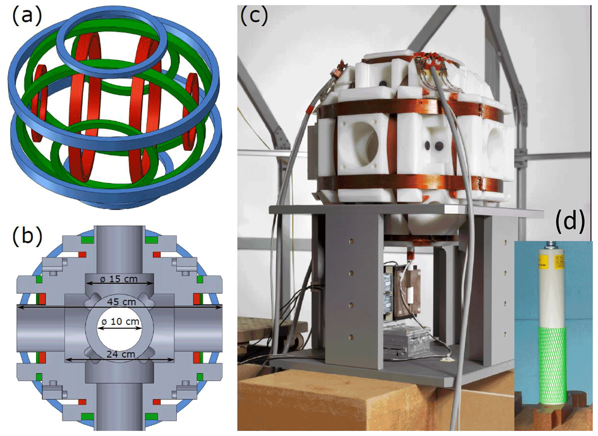
Figure 1 3D compact coil system based on two split-pair coils with (a) showing a sketch of the winding packages labeled in red, blue and green for different axes. A technical drawing of the coil frame including inner dimensions for experimental space is presented in (b). A picture of the final 3D coil system including holder and translation stages for sensor movement below the frame is shown in (c). Inset (d) shows the 3D fluxgate sensor for field characterization.

Table 1 Center points of winding packages (X,Y,Z), radius r, and distance a to the field center at (0,0,0), as well as number of layers n_r and windings per layer n_a.

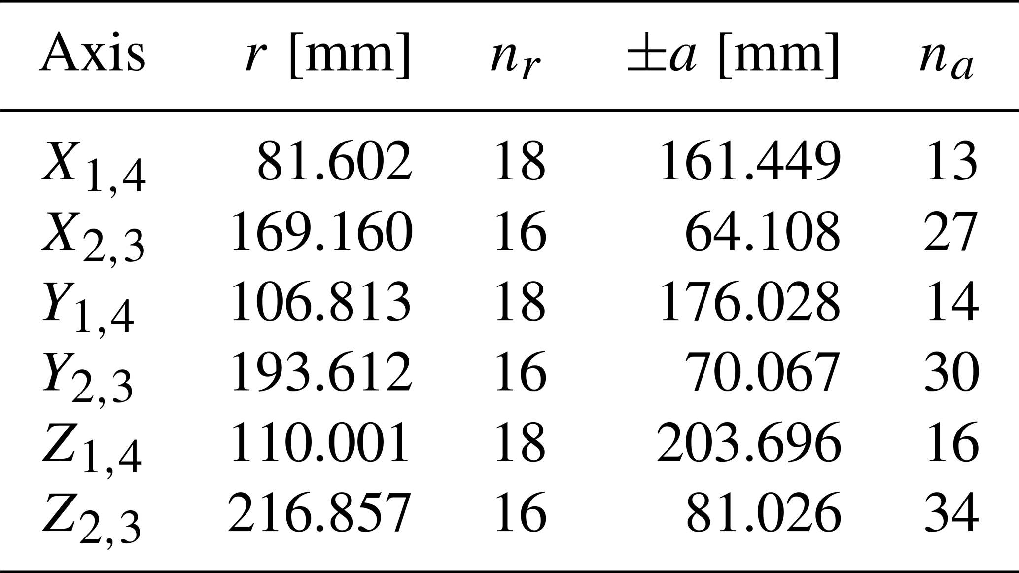
The final parameters for r, n, and a are summarized in Table 1. We obtained a homogeneity of 10⁻⁶ within the inner 10 % of the coil diameter in the optimization process, as shown in Fig. 2a and b for the flux density component B_z and B_y in the y plane, respectively. The homogeneity deviates from the ideal Braunbek configuration by 2 orders of magnitude (Braunbek, 1934; Ludke et al., 2007). We know from long years of experience in coil manufacturing and winding that typical fabrication tolerances of individual coil parts limit the final homogeneity of the generated magnetic field in a comparable order of magnitude. In measurements of the final coil dimensions, strain-induced distortions from circular shapes caused by the winding process were not detected. The gradient field has been optimized to be linear in contrast to a Braunbek system.

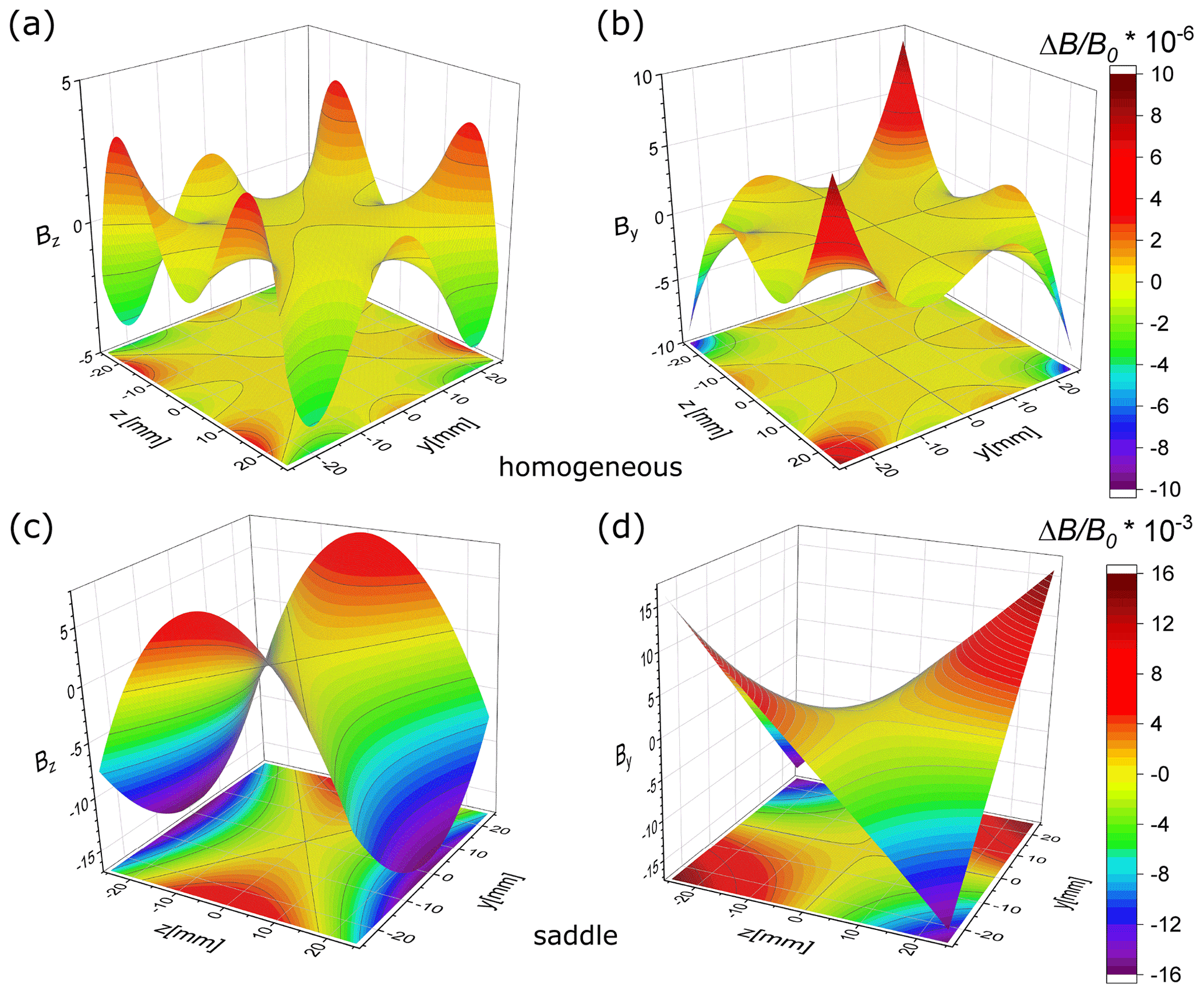
Figure 2 Calculated relative flux densities $\frac{\mathrm{\Delta }B}{B}$ in the zy plane for optimized coil parameters are shown for B_z in (a) and B_y in (b), respectively. Relative values for B_z and B_y when currents are reversed for saddle field configuration are displayed in (c) and (d).

Figure 2c and d show relative field values B_z and B_y for the saddle configurations, i.e., the direction of the current in the two outermost winding packages is reversed, giving rise to two maxima in the magnetic flux density.

As seen in Fig. 1, the coil body is manufactured out of one piece of polyoxymethylene (POM-C). This material provides physical stability and it is easy to machine. The axles are manufactured from the inside out on a turning machine and wound with the copper wire. Finally, the coil body rests on a holding frame. Special non-magnetic translation stages (see Fig. 1c) are located below the coil for the movement of the sensors.

3 Measurements with NMR

All characterization measurements are carried out within the Physikalisch-Technische Bundesanstalt (PTB)'s active EMF compensation (Zikmund et al., 2015b), which reduces the local EMF value of about 49 µT to a background field of less than 20 nT. We use an NMR technique on protons, and the free induction decay (FID) on water samples (Slichter, 1996; Harcken et al., 2010) to measure the scalar magnetic flux density B generated by the 3D coil system. The NMR probe consists of a 40 mm glass sphere filled with highly purified water. It is placed inside the field center, averaging the field signal B effectively over the entire probe volume.

3.1 Coil constants

The coil constants $k_{x,y,z}=\frac{B}{I_{x,y,z}}$ measure the ratio of the flux density B in respect to the generating currents $I_{x,y,z}$. The currents are estimated via a voltage measurement (Keithley 2002) on a calibrated shunt resistor. All three coil axes ($x,y,z$) are measured individually at a flux density of 1 mT. The measurements are carried out multiple times and with reversed current directions producing fields ±B to eliminate the influence of the final background EMF. Table 2 summarizes our results.

Table 2 Coil constants obtained for each axis ($x,y,z$) including uncertainties according to BIPM et al. (2008) on a confidence level of 95 % (last two digits).

The uncertainty of the measurements is dominated by the uncertainty of the current. Furthermore, contributions from the positioning of the sample in the field center and the area of homogeneity need to be taken into account.

3.2 Angles between coil axis

Manufacturing the coil body from one piece of material results in coil axes that are almost perpendicular to each other. Nevertheless, unavoidable deviations from ideal dimensions due to machining tolerances need to be estimated and included into correction terms in order to precisely generate magnetic field vectors with the 3D coil system. We use a scalar method to determine those deviations. Due to the compensation, EMF can be neglected.

To measure the angle between two coil axes, both coils are excited with similar currents, I_x and I_y, producing a diagonal vector field ${\overrightarrow{B}}_x+{\overrightarrow{B}}_y$. The scalar value $B_{\mathrm{NMR}}=|{\overrightarrow{B}}_x+{\overrightarrow{B}}_y|$ is measured via the FID NMR technique. Based on equation

$$\begin{array}{}\text{(1)}& B_{\mathrm{NMR}}^{\mathrm{2}}=({\overrightarrow{B}}_x+{\overrightarrow{B}}_y{)}^{\mathrm{2}}={\left(\begin{array}{c}{k}_x{I}_x+k_y{I}_y\cos \mathit{\alpha }\\ k_y{I}_y\sin \mathit{\alpha }\\ \mathrm{0}\end{array}\right)}^{\mathrm{2}},\end{array}$$

and known coil constants k_x,y, we estimate the angle

$$\begin{array}{}\text{(2)}& \mathit{\alpha }={\cos }^{-\mathrm{1}}\left({\displaystyle \frac{B_{\mathrm{NMR}}^{\mathrm{2}}-(k_x{I}_x{)}^{\mathrm{2}}-(k_y{I}_y{)}^{\mathrm{2}}}{\mathrm{2}{k}_x{I}_x{k}_y{I}_y}}\right)\end{array}$$

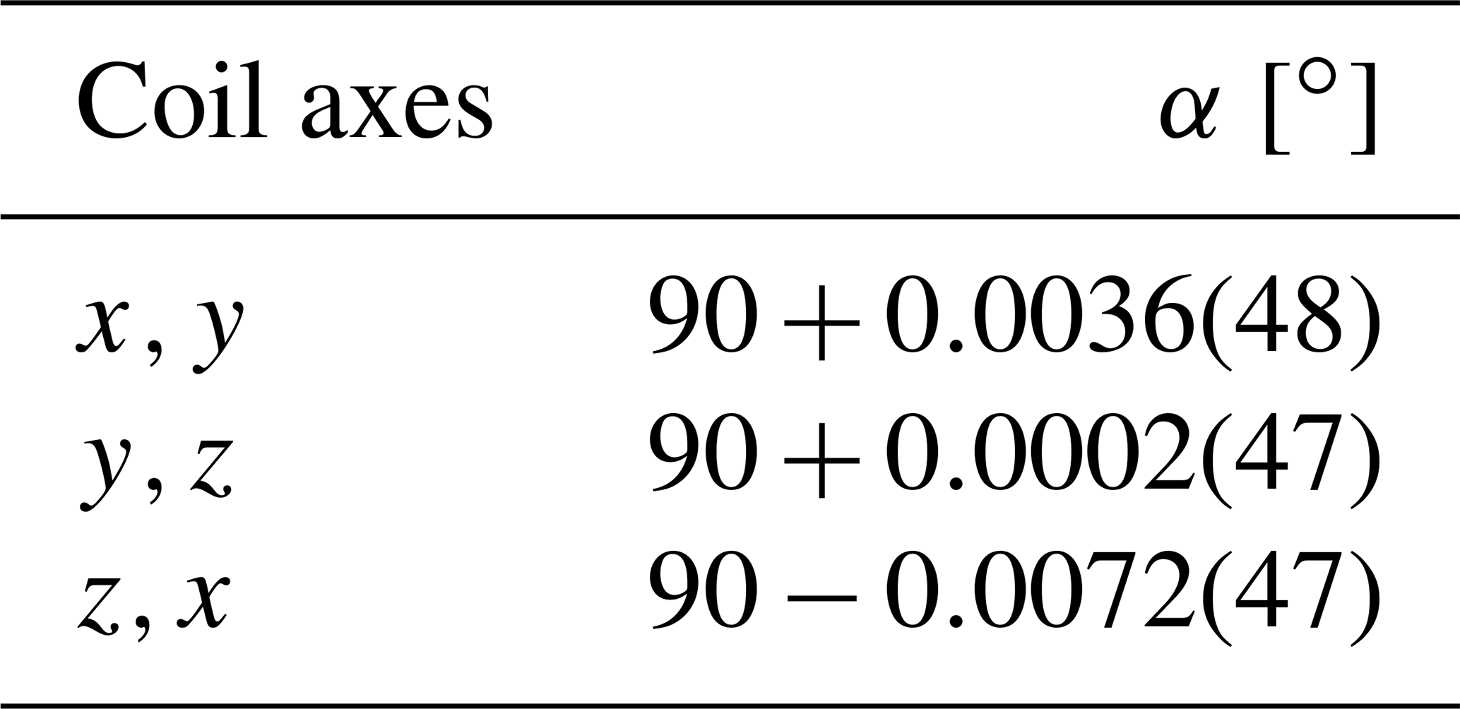
between the coils along x and y direction. The same procedure is carried out for the other angles between y,z and z,x, respectively. Table 3 lists the final results. Our 3D coil system has small misalignment angles in the order of millidegree, which affirms the chosen 3D coil layout.

Table 3 Angle α between two axes of the 3D coil system with uncertainty on a confidence level of 95 % (last two digits).

4 Field scans

Finally, we test the magnetic flux density distribution by performing sensor scans in a defined volume at the field center. The movement is done by means of three orthogonal translation stages (MT105-NM from Steinmeyer Mechatronik) made of non-magnetic material. Sensors with weight less than 2 kg can be moved ±25 mm in all three directions. We utilize both a commercially available 3D fluxgate sensor (Foerster GmbH) and a self-developed 3D Hall device to conduct homogeneity scans. The fluxgate magnetometer features the following dimensions: the saturation cores for each spatial direction are duplicated and arranged to form a common center point and each core has a total length of about 2 cm, causing a large sensitive volume of the magnetometer and leading to an averaging effect over about (2 cm)³. In contrast, the Hall device consists of three individual Hall elements placed on each side of the corner of a glass cube covered in reflective coating. The sensitive volume of the Hall cube is less than 1 mm³ (Rott et al., 2020). The mirror surfaces allow the external referencing of the tilting and positioning of the cube (Rott, 2021).

In general, the position of a magnetic field sensor can be determined with a 3D coil system by varying the currents in individual winding packages, leading to different distributions of the magnetic field. The simplest version is a gradient field with reversed currents in winding packages of one coil of a split pair in respect to its counterpart. In gradient configuration, a scalar magnetometer detects only a field minimum in the center, whereas a vector magnetometer detects ±B values with zero crossing. Furthermore, each individual sensor along three different spacial directions resolves a gradient field, which allows it to position itself in a 3D space, and not just along one main axis.

One needs to keep in mind that three individual sensors in a 3D magnetometer have finite dimensions and are not located at one identical point. Therefore, one needs a more complex magnetic field distribution than the simple gradient field in order to determine the exact position of each individual sensor. We introduce the saddle field as calculated from the 3D coil parameters and shown in Fig. 2c, d.

4.1 Homogeneous field

The cylindrical body of the fluxgate magnetometer was positioned concentrically in the opening of the 3D coil system measuring along the z axis. The z position of the sensor (axial) in the cylinder was centered accordingly to the manufacturer's specifications. Due to the restricted field range of the magnetometer, a flux density of 100 µT was applied in an alternating way to all three axes. Figure 3a and b show a section of the z-axis results for x=0 mm of the B_z and B_y values, respectively. While being mostly constant in the order of 10⁻⁵, the axial B_z values exhibit a slight saddle. The B_y results reveal additional tilting of the fluxgate magnetometer. We can not rule out that this happens due to the high mass of the device pulling on the translation stage and causing misalignment angles of less than 100 µrad. The latter leads to changes in B_y by $\mathrm{1}\times {\mathrm{10}}^{-\mathrm{4}}$. We are able to compensate the effect by averaging over opposite moving directions.

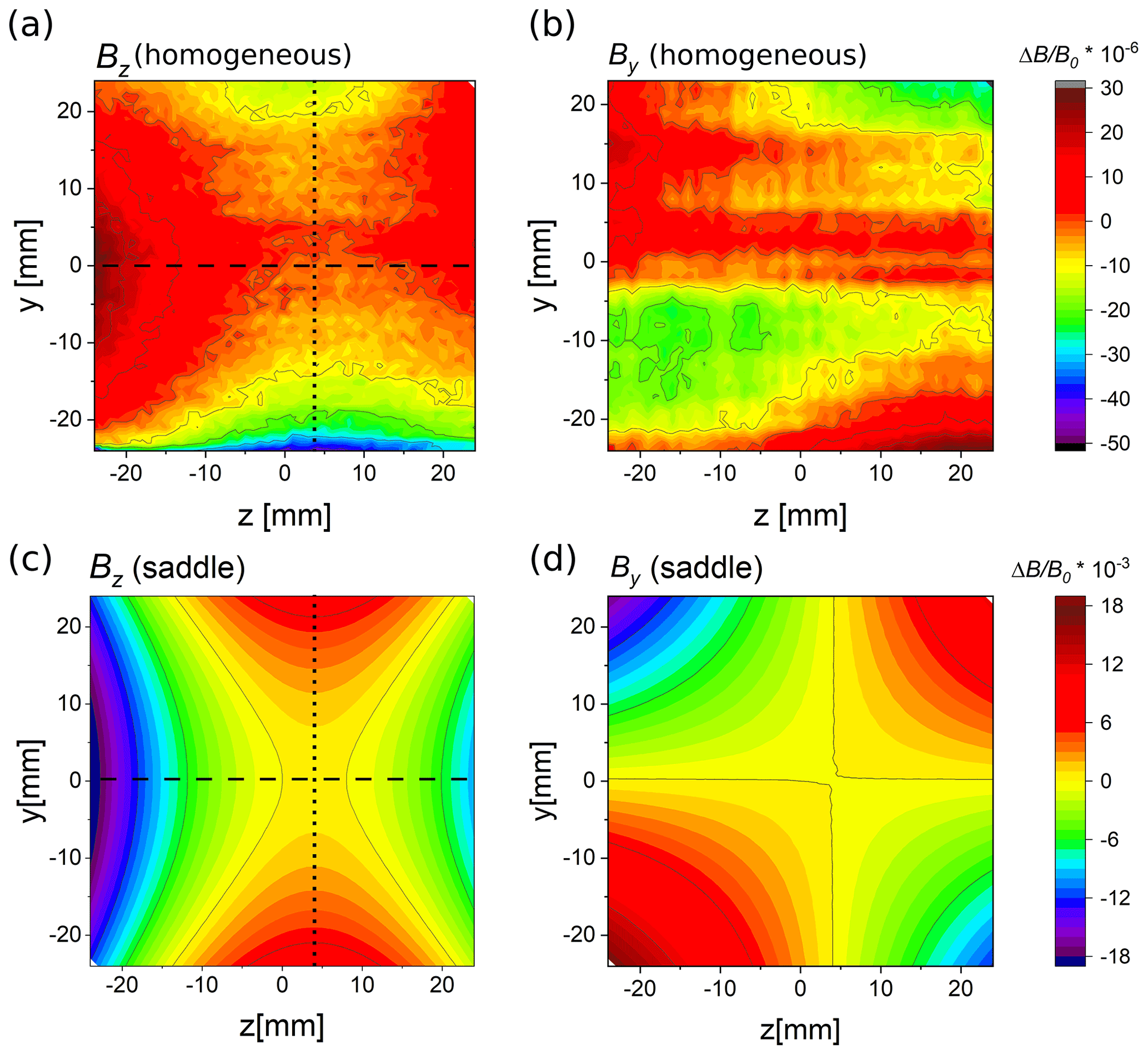
Figure 3 Measurements of the flux densities along the z axis. Data for homogeneous field distribution relative to the coil center in parts per million are shown in (a) and (b). The same values for the saddle field configuration are exhibited in (c, d). The axial components for B_z are shown in (a) and (c), whereas (b) and (d) display the radial contribution B_y. Dashed and dotted lines correspond to Fig. 4.

In our measurements we found a homogeneity better than $\mathrm{5}\times {\mathrm{10}}^{-\mathrm{5}}$, relative to the axial flux density at the center B₀ inside a volume sphere with a diameter of 45 mm. Note that the sensitive volume of the fluxgate sensor is about 20 mm³, which causes an averaging effect on the experimental data. Further investigations with a magnetometer, having comparable sensitivity but higher spacial resolution, are necessary to confirm the field characteristics obtained here. In Fig. 4a, b, the measured axial and radial flux densities of the B_z component are compared with theoretical values. It should be possible to further improve the performance of the 3D coil system by applying a minimally smaller current on the two outer winding stacks, e.g., by means of bypass resistors. In this way, the minimal saddle could be removed. Nevertheless, we consider the achieved homogeneity of the 3D coil system as satisfactory.

4.2 Saddle field

As already mentioned, a saddle field with quadratic change of the flux density in the coil center can be obtained by changing the current direction in the outer winding packages. The analytic expression along the z-axis

$$\begin{array}{}\text{(3)}& {\overrightarrow{B}}_{\mathrm{S}}(x,y,z)=\left(\begin{array}{c}\mathrm{0}\\ \mathrm{0}\\ B_{\mathrm{S}}\end{array}\right)+a_{\mathrm{S}}\left(\begin{array}{c}\mathrm{2}xz\\ \mathrm{2}yz\\ x^{\mathrm{2}}+y^{\mathrm{2}}-\mathrm{2}{z}^{\mathrm{2}}\end{array}\right)\end{array}$$

describes a saddle point B_S in the center with axial decrease and radial increase of flux density with farther distance in the x,y, and z directions (Rott, 2021).

Magnetic flux density in the shape of a saddle can be resolved in the experimental data as seen in Fig. 3c, d, however, the midpoint is shifted by about 4 mm along the z axis. We attribute this to a slight displacement of the sensitive volume inside the sensor case. For direct comparison, Fig. 4 shows experimental and calculated values of B_z along the indicated dashed and dotted lines in Fig. 3. In panels c and d, measurements with a 3D Hall device are added. For the Hall probe, the sensitive volume, and therefore the average dimension, is smaller than the distance between points. We observe good matching between calculation and experiment for the saddle configuration and larger deviations for the homogeneous current feed to the 3D compact coil. The latter result is caused by a large sensitive volume of the fluxgate magnetometer.

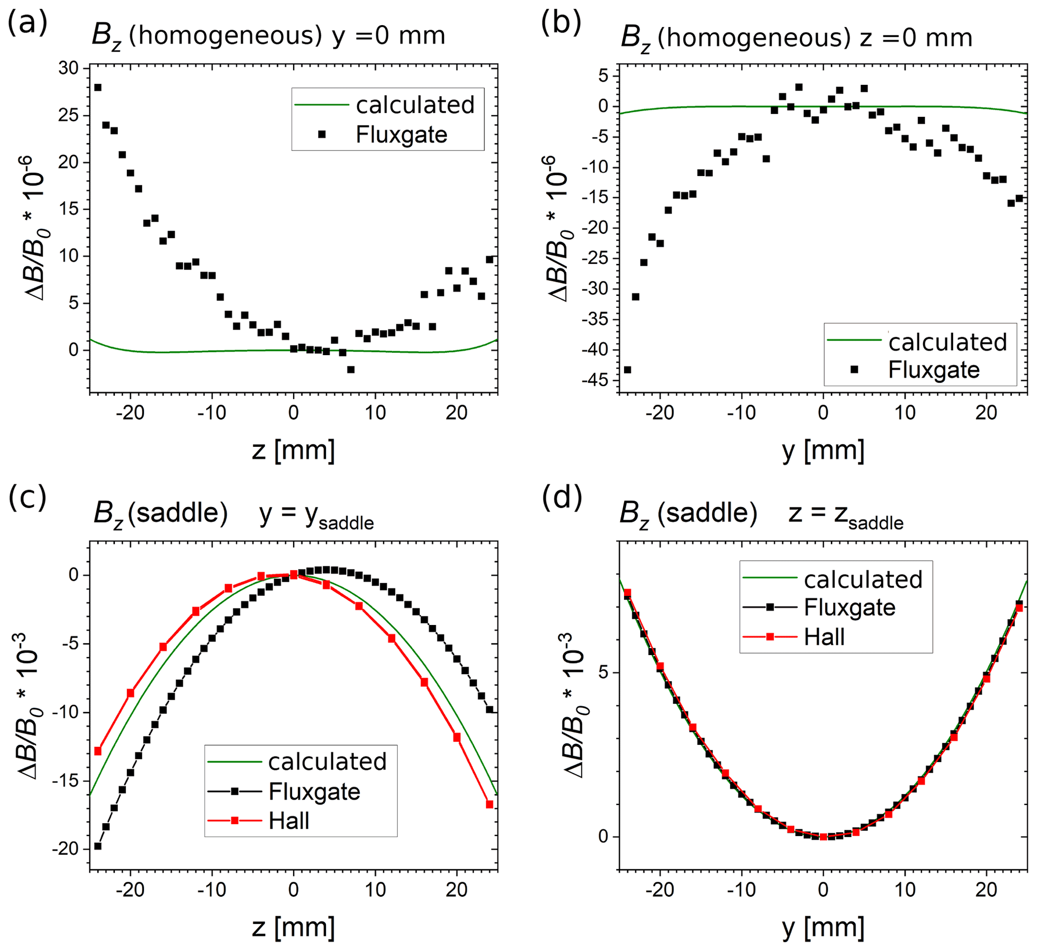
Figure 4 Direct comparison of experimental and theoretical results for homogeneous (a, b) and saddle field configuration (c, d) for selected data points as marked in Fig. 3a, and (c) by dashed and dotted lines. The experimental data were obtained by fluxgate measurements, and for the saddle field configuration in (c) and (d), complemented by Hall sensor data.

For each component ($i=x,y,z$) of a 3D sensor, the following relation describes the sensor position in the field of Eq. (3):

$$\begin{array}{}\text{(4)}& B_i={\overrightarrow{n}}_i\cdot {\overrightarrow{B}}_{\mathrm{S}}(x-x_{\mathrm{0}},y-y_{\mathrm{0}},z-z_{\mathrm{0}}),\end{array}$$

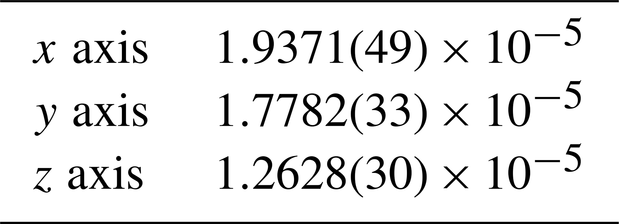
where n_i is the normalized vector of the respective sensor element. It has two degrees of freedom resulting in two free parameters. The position of the 3D sensor is labeled by x₀,y₀, and z₀. Together with the parameters B_S and a_S, the saddle field can be described by seven parameters. We chose suitable initial conditions to fit the model to the experimental data. The fit works best for the normalized vector (n_i) pointing in the same direction as the involved coil axis. Table 4 summarizes the obtained saddle parameters (a_S) for all three axes. The flux density at the saddle point is about 75 % of the one in the homogeneous field in all three axes.

Table 4 Parameter a_S experimentally determined by 3D Hall sensor measurements with double standard uncertainty, e.g., last two digits.

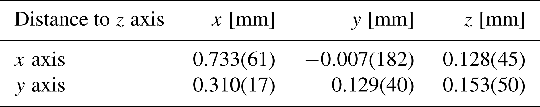
The saddle points of the individual coil axes are not necessarily at the same location, therefore, we used 3D Hall probe data with the exact known sensor positions, i.e., Eq. (4), to estimate the displacements relative to the z axis. Results are given in Table 5.

Table 5 Deviation of the position of the saddle points in x and y direction in respect to the z axis. Uncertainties are determined with a confidence level of 95 % (last two digits).

If one assumes that the coil axes of the saddle fields have a similar misalignment of axes as in the homogeneous field configuration, the deviations of midpoints can be converted into an absolute coordinate system. Calibrations of unknown 3D magnetometers benefit from this capability. The position of individual sensor elements of the magnetometer can be determined relative to each other. We tested this option with the fluxgate magnetometer and found that the positions of the sensors were less than 0.2 mm apart.

5 Summary

We calculated, built and tested a compact 3D coil system based on double split coils that can be used to generate magnetic flux densities up to 2 mT, pointing in any arbitrary direction. During layout of the system, a genetic algorithm was used to optimize the coil parameters. We found that precise manufacturing is crucial to reach the desired specifications for the 3D coil system. We obtained a relative homogeneity $\mathrm{\Delta }B/B={\mathrm{10}}^{-\mathrm{6}}$ in the center volume of roughly 2 cm along each direction in accordance with calculations.

The 3D coil system is suitable for calibrations of vector magnetometers, but needs further in-depth characterization. So far, values of magnetic flux density vectors are traceable to SI standards. In a next step, the magnetic field vector should be linked to an orthogonal reference frame for traceability of sensor position and angularity. The homogeneity of individual axes of the 3D coil is approximately known. The position of individual sensor elements can be determined by means of an inhomogeneous current feed to the 3D coil system, specifically gradient and saddle field configurations.