Structure of digital metrological twins as software for uncertainty estimation

Ongoing digitalization in metrology and the ever-growing complexity of measurement systems have increased the effort required to create complex software for uncertainty estimation. To address this issue, a general structure for uncertainty estimation software will be presented in this work. The structure was derived from the Virtual Coordinate Measuring Machine (VCMM), which is a well-established tool for uncertainty estimation in the field of coordinate metrology. To make it easy to apply the software structure to specific projects, a supporting software library was created. The library is written in a portable and extensible way using the C++ programming language. The software structure and library proposed can be used in different domains of metrology. The library provides all the components necessary for uncertainty estimation (i.e., random number generators and GUM S1-compliant routines). Only the project-specific parts of the software must be developed by potential users. To verify the usability of the software structure and the library, a Virtual Planck-Balance, which is the digital metrological twin of a Kibble balance, is currently being developed.

1 Introduction

With the increase of the complexity of measurement systems, the determination of measurement uncertainties using a conventional uncertainty budget, as described in the GUM (JCGM, 2008a), is often not possible or may lead to unrealistic results. In these cases, the Monte Carlo (MC)-based method described in GUM S1 (JCGM, 2008b) is applied.

To meet the requirements of the continuously evolving field of coordinate metrology, the Virtual Coordinate Measuring Machine (VCMM) was developed. Using the MC approach, the VCMM has made it possible to consider significant coordinate measuring machine (CMM) deviations caused by the guideway geometry and the probing system, among other effects (Wäldele and Schwenke, 2002; Heißelmann et al., 2018). The previously used methods were not suitable or were far too time-consuming for practical application. The VCMM is used by DAkkS-accredited laboratories as well as in the planning and evaluation of measurements in industrial quality control.

The Planck-Balance (PB) (Rothleitner et al., 2018), a tabletop version of a Kibble balance (Robinson and Schlamminger, 2016), is currently under development at PTB and TU Ilmenau. Similarly to the VCMM, within the PB, the individual effects interact in a complex manner. Because these effects cannot be separated, it is not possible to describe them using a conventional uncertainty budget. The Virtual Planck-Balance (VPB) currently under development is designed to allow major uncertainty contributors (e.g., the Abbe error) to be considered correctly.

The aim of the work presented here is to provide a structure for MC-based uncertainty estimation software that can be used to guide the design and the implementation for new systems. To this end, the structures of an already established tool that is used to estimate metrological uncertainty were analyzed and generalized. The VCMM was considered for this purpose.

Different projects in which the MC approach is used for uncertainty estimation naturally share similar code. However, because it has not been possible to reach a consensus on which tools and structures should be used to create MC-based software, commonly found software components are constantly being reprogrammed. As a consequence, the effort required to develop such software increases along with the possibility of errors. Individual projects use different approaches to solve the same problems and distinct wordings to describe similar concepts. These factors complicate communication between organizations and projects and slow down overall development in this field.

To address the issues listed above, a supporting software library is currently being developed. The library is written in a portable and extensible way using the modern C$++$ programming language. It provides a set of reusable tools which can be used to describe any metrological system in a compact and maintainable way. The library was developed based on the structures used by VCMM, and it implements GUM S1-compliant routines for uncertainty estimation.

During the development of new simulation software, the general idea is to split up a complex system into a number of simpler software modules, where each module is based on a single physical effect. The individual modules are then combined to represent the whole measurement process. By embedding the complete measurement model into a MC simulation, the uncertainty estimation is carried out. The VPB was chosen as a first practical example to be developed using the proposed software structure and the supporting software library.

Additionally to the tools necessary to model the measurement process itself (e.g., the random number generators), the library also provides a variety of utility tools to set up an adaptive MC simulation to evaluate the uncertainties and to analyze the system properties by means of sensitivity analysis. Some of these functionalities were adapted from the general software structure, and some were added for completeness.

In the next section, the VCMM concept will be introduced and used to derive a general software structure for uncertainty estimation software. An overview is given of the elements of the VCMM software that can be reused for other projects. The generalization process for the VCMM is described in Sect. 3. From the metrological point of view, the traceability of simulation results is of key importance. To go from “simulation software” to a traced digital metrological twin (D-MT) as proposed by Eichstädt et al. (2021), a series of requirements must be met; these are listed in Sect. 4. The components of the supporting software library and a description of certain technical aspects will be presented in Sect. 5. Section 6 will demonstrate how an actual software module is created using the supporting software library. The current gravitational acceleration model of the VPB will be used as an example.

2 VCMM concept

In the VCMM, MC-based simulation software is used to determine the uncertainties of a dedicated measurement task that is performed by means of a specific coordinate measurement machine. The concept of the VCMM is based on the notion that the process of the real measurement is recreated in a simulation. The simulation can then be repeatedly carried out to estimate uncertainties using the data from a single measurement along with additional information known a priori. The influence of the uncertain input quantities is considered by means of mathematical models that describe the disturbance of the measured data. For each simulation step, the models are repeatedly evaluated, and the disturbance is added to the data from the real measurement. The output quantities are calculated based on the disturbed data. The result consists of an estimate taken directly from the evaluation of the measured data and an uncertainty obtained by means of a statistical analysis of the disturbed (i.e., simulated) data.

As described by Heißelmann et al. (2018), the VCMM consists of multiple models that describe the positional deviation of the measured coordinate points. Each model is implemented as a separate software module. When combined to a single piece of simulation software, the modules propagate the influence of multiple input quantities on measured quantities (i.e., output quantities) that include distances, diameters, and angles. For the evaluation of the output quantities, the same fit algorithms are used for the simulated data and the real data; these algorithms are provided by the software of the CMM.

Because this approach uses the measurements' disturbances, which are caused by uncertain influence quantities, there is no strict need to recreate the entire measurement within the simulation; only models describing the influence of the uncertain input quantities on the output quantities should be considered.

3 General D-MT structure

In order to provide a generalization of the structures used by VCMM, its source code, which consists of roughly 40 000 lines of code, was reviewed and characterized. Additionally, a lightweight version of the VCMM was implemented from the ground up. This version includes all the major modules needed in order to perform comparison evaluations using data from real measurements. Newer developments (i.e., scanning and the CMM rotary table) were not considered.

It was observed that the internals of the VCMM can be subdivided into three main parts: modules, which encapsulate individual physical models, random number generators (RNGs) and statistics, and support components. Depending on the role and generality of given software components, only some of these can be considered for future reuse.

The VCMM models and its support components (e.g., XML configuration file readers) make up around three-quarters of the total code share. They cannot be considered to be generally reusable for other projects, as they are very specific to the VCMM itself. However, the RNGs and statistics are required by all MC-based software programs used for uncertainty estimation; these were implemented as a stand-alone library, named vmlib, that will be discussed in Sect. 5.

The new implementation of the VCMM consists of roughly 5 times fewer lines of code than the original software. The drastic reduction in code size was possible due to the well thought out design of the individual modules and by extracting the RNGs and statistics into the supporting library. The usage of a third-party library for linear algebra (Guennebaud et al., 2010) helped a lot to reduce and simplify the code within the modules. It should be noted that because the re-implementation of the VCMM does not include all the original functionalities, no direct comparison should be made. However, it can be seen that the size of the VCMM (and thus its complexity) can potentially be reduced.

The investigation of the re-implementation of the VCMM was geared toward analyzing patterns in which the RNGs are used to build individual modules and how the statistical components connect them to a single piece of simulation software. Figure 1 shows the general structure derived from this investigation. The structure should be read from the left to the right – in the same order the simulation is performed. The entire structure is enclosed by a simulation loop that denotes the repeated evaluation of the components within the MC simulation.

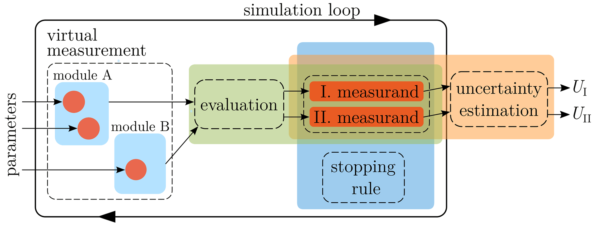
Figure 1 Proposed structure of D-MTs for uncertainty estimation, derived from the generalization of the VCMM.

Before the simulation starts, the RNGs (depicted as red circles) of the individual modules are parameterized from external sources such as XML files. The modules are contained inside the virtual measurement component, whose task is to replicate the real measurement process; it is the aggregate of individual modules mentioned before. On each run of the MC simulation, the virtual measurement produces a dataset that could have been obtained from a real measurement. Next, the data are passed to the evaluation algorithm. It is supposed to be the same algorithm which is also used to evaluate the real measurements. As the evaluation result, a new value is obtained for each simulated quantity. While the simulation process is being carried out, the results of the individual evaluations are stored inside the measurands. A measurand is a programmatic representation of a real measurement quantity. It stores the results of the individual simulations for the future uncertainty estimation, which is performed after the execution of the MC loop is complete. The uncertainty estimation is performed for each measurand.

The stopping rule is an optional component that can be used to achieve a given numerical tolerance or to prematurely abort the simulation. During the simulation, the stopping rule observes the numerical properties of the individual measurands and signals to the simulation loop whether the simulation should be continued or stopped.

4 Requirements

So far, the presented structure is intended to guide the development of new software for uncertainty estimation, i.e. a digital twin (DT). However, to be used in a traceability chain, the results of the given DT must be metrologically traced, thus making it a digital metrological twin (D-MT). The term “digital metrological twin” was explicitly introduced by PTB (Eichstädt et al., 2021) to clarify its affiliation to metrology, as the definitions of “digital twin” may differ significantly depending on their application (Glaessgen and Stargel, 2012; Negri et al., 2017).

In Eichstädt et al. (2021), a definition and requirements for a D-MT are given. It states that “the measurement uncertainty [must] be calculated according to valid standards”. This requirement is automatically covered, as the supporting software library implements the GUM S1 uncertainty estimation routines, which are considered as a state-of-the-art method.

Further it states that to achieve a traced simulation result, “all input parameters [must be] determined traceable and [must be] stated with corresponding measurement uncertainty”. Regarding this requirement, it should be noted that a measurement process described by means of a proposed software structure does not automatically become a D-MT. The developer of such software has no influence if the input parameters used for the simulation are metrologically traced or not. This aspect lies completely in hands of the software user.

Lastly, Eichstädt et al. (2021) state that the results of such simulation software, to become a D-MT, must be “validated by traceable measurements”. This aspect lies more in the hands of the scientist who develops the mathematical models for a given measurement process. The actual software developer is responsible for correctly implementing a given mathematical model and integrate it with the surrounding components.

In the following, some aspects around the validation of the software and the traceability of its results are discussed in more depth.

4.1 Models

Models used by the D-MT must be well understood, verified, and documented. The scope of the individual models should be defined. The full scope of the D-MT is derived from the intersection of the scopes of all its models and should be clearly communicated to the end user of the system.

The simulation results produced by the virtual measurement must have statistical properties that are similar to those of the real measurements. All the main uncertainty components of the real measurement device and process must be identified and considered in the simulation. Systematic errors, which are not always visible in the measured data, should be identified and considered. Additionally, when the averages of the input quantities are shifted, the models must respond similarly to the behavior of the real measurement. The boundaries of the shifts must be included in the scopes of the models.

4.2 Validation

The evaluation algorithm of a measurement setup can often be nontrivial and difficult to implement. It must be well tested to guarantee its correctness. For the testing, different scenarios can be implemented. When an algorithm is implemented “from the ground up”, the unit testing approach is recommended; see, e.g., Beck (2002). If applied thoroughly, most of the difficult-to-perceive errors can be eliminated.

Both the individual components and the results of the entire D-MT must be validated; reference datasets can be used for this purpose (Forbes et al., 2015). In coordinate metrology, a web service, TraCIM, has become well established (Wendt et al., 2015). The service is being continuously expanded to include new algorithms both from coordinate metrology and from other fields of metrology.

This validation can also be performed by means of intercomparison measurements and by comparing the results of our software to the results of reference software and to the results of other D-MTs. Additionally, the simulated measurement results can be compared to the statistics of a series of repeated real measurements. This latter approach may not cover systematic errors that occur only on timescales larger than those of the actual measurements or only between the different measurement setups. Section 6 provides an example of how systematic effects are accounted for in a simulation.

5 Supporting software library

To make the creation process for new software for uncertainty estimation efficient and less error-prone, a supporting software library named vmlib is currently being developed. The library is implemented in the C$++$17 programming language and is designed to make it easier for users to implement the structure from Fig. 1.

Each component shown in Fig. 1 is covered by the vmlib library. For example, the measurand component is represented by a vm::measurand class, which can be easily integrated with a vm::stability object, which is used for adaptive MC. It also implements the RNGs by means of a vm::random_value class and provides a functionality for GUM S1-compliant statistical evaluation.

5.1 Random number generation

RNGs are the most complex components of the software library. They are also intended to be the most common software components in the software written by the users themselves with the aid of the library, as they are used within the models to represent the uncertain input quantities of the measurement process.

Generally, RNGs can be used with all kinds of univariate probability density functions (PDFs). However, for our purposes, PDFs that can be fully described in terms of their mean and the standard deviation are of special interest. In the following, we refer to this set of PDFs. These PDFs can be treated as a group of polymorphic objects that are parameterizable by means of two values. For the sake of convenience, RNGs containing this type of PDFs are called polymorphic RNGs. The restriction mentioned above allows the individual RNGs to be parameterized using the data containing the name of the distribution (e.g., normal or uniform), its mean, and the standard deviation. The library provides a set of runtime objects that are used to dynamically create RNGs. The same runtime objects are used when the RNG parameters are first read from the configuration files.

As the aim of the VCMM concept is to recreate the measurement process in the most realistic way possible, one must distinguish the timescales on which a given input quantity acts. In the simulation, the different timescales are replicated by means of nested simulation loops; here, the outermost loop is the main MC loop, which is the realization of the outermost timescale. This is necessary to correctly consider the influence of the systematic effects on the resulting uncertainties.

The RNGs provided by the library are designed to simplify the creation of a simulation containing multiple timescales. These RNGs can store their current random value until an explicit request has been made to generate a new one. For this purpose, the RNG interface provides three methods. The randomize() method generates a new random value from the underlying PDF; it internally stores the result without returning it. The random() method generates, stores, and returns a new random value. The stored() method returns only the previously generated random value without generating a new one. The exact names of these methods are not final and may change in future versions of the library.

These methods allow the point in time at which a new random value is generated to be clearly distinguished from the point in time at which it is used for a computation. The library has borrowed this approach from the VCMM's RNGs and re-implemented it in a modern and efficient way. Without this functionality, it would be necessary to introduce additional variables in order to store the current value and the state of the execution order – a manual approach that is unsuitable for large applications.

The core components of RNGs are implemented as proposed by Polishchuk (2020) with additional extensions. This means that RNGs are highly customizable and can be adapted to meet project-specific requirements. For example, using the preprocessor definitions, any floating-point type can be set for the numbers generated by the RNGs. Furthermore, any random engine from the <random> header (e.g. std::mt19937 or std::knuth_b) can be used. The engine can be seeded using a custom sequence of constants or using a time-based seed. The implementation of the time-based seed was taken from Polishchuk (2020).

For all customization aspects of the library, user-provided solutions can be used, provided that these solutions implement the interface required by the C$++$ standard or by the documentation of the library.

5.2 Registry

For the PDFs mentioned in the section above, the library implements the shifted delta distribution. This distribution is described in terms of a mean and a second number that is always replaced by zero (as it is irrelevant for a given distribution). This distribution is special in the sense that it allows the “yet-not-uncertain” input quantities to be described in the same way as the regular (i.e., uncertain) input quantities. It allows an input quantity to be prematurely treated as random but only later to be parameterized with a non-δ distribution.

The properties of polymorphic RNGs allow any distribution to be converted into the δ distribution during runtime. Thus, the “randomness” of the distribution will be disabled. To this end, a special tool set is provided by the vmlib library.

This functionality is realized by so-called registry objects. Such objects form a bookkeeping mechanism containing the unique name of an input quantity and its address in the memory. At any time during the MC simulation, a specific RNG can be referred to by its name; then, its properties can be varied or its randomness entirely disabled.

Additionally, a group of multiple RNGs can be united to form a single entry inside the registry object. This makes it possible to disable the randomness of multiple quantities at once.

5.3 Sensitivity analysis

When multiple complex models interact with each other, the uncertainty contributions of the individual quantities are not easy to distinguish. However, this information is essential to understanding the behavior of the system and finding its main uncertainty contributors.

Using the registry objects described in the previous section, a variety of tools for analyzing the system properties can be created. These could include parameter sweeps or even inverse solvers. As a proof of concept for future developments, a variance-based tool for conducting a sensitivity analysis is provided by the library. This tool determines the contributions of the individual input quantities to the total variance of an output quantity.

The analysis is performed as follows. First, a simulation is performed in which all uncertain quantities are “active” (i.e., they produce random values). In this way, the total variance of the output quantity is computed. Next, the MC simulation is repeated once for each input quantity; here, only one quantity is active at a time, while all other quantities are disabled. Ratios are formed of variances from simulations with individual (active) input quantities to the total variance. These ratios then constitute the percentage contribution of the individual quantities to the total variance. The same analysis can also be performed with groups of multiple input quantities.

It is known that the drawbacks of this simple approach to sensitivity analysis include its linear time complexity and the fact that it provides incorrect results for highly nonlinear systems. However, the tool has already proved its usability in the early development stage of the VPB. It is available for any system created using the given library; only very little additional code must be added to carry out a sensitivity analysis, even for complex systems. Due to its drawbacks, the tool should be used with care. In the future, it will likely be possible to create more sophisticated sensitivity analysis tools using the functionality of the registry objects. Allard and Fischer (2018) describe other approaches to sensitivity analysis that may be considered.

5.4 Measurands, stopping rule, and uncertainty estimation

The results of the individual runs of the simulation loop are stored inside the measurand object. Each simulated quantity requires a separate measurand object. This object is a “wrapper” around the std::vector class and stores additional information about the measurand such as its name and the index. The measurand object provides an interface that allows the “stopping rule” to access its current statistical properties. To make these data accessible on each execution of the simulation loop, an algorithm for the running average and the running standard deviation is implemented inside the measurand class. This leads to a slight increase in the computational effort; however, this is negligible in comparison to re-computation using a naive implementation.

Statistical information for individual output quantities can be accessed by the stopping rule in each simulation run. Based on the underlying algorithm, a decision is made concerning how often the simulation must be repeated. The library currently implements the stopping rule defined in GUM S1. As shown by Wübbeler et al. (2010), the GUM S1 method has a comparably low probability of successfully predicting the number of repetitions necessary to achieve a desired numerical tolerance. The same paper proposes a two-stage procedure created by Stein (1945) as a possible replacement of the method currently implemented.

The library provides GUM S1-compliant routines for uncertainty estimation. These include functions for the computation of the probabilistically shortest coverage intervals and the symmetric coverage intervals, where the desired coverage probability could be given as an optional argument. As a default, a coverage probability of 95 % is used. Additionally, the basic statistical properties of the output quantities (i.e., the number of simulation runs, the mean, and the standard deviation) can be directly accessed from the measurand objects after the simulation is complete; no additional computations are required.

5.5 Parallelization

An MC simulation can easily be performed as a parallel computation, as there are almost no dependencies between the individual evaluations. Synchronization is only required to protect the RNGs along with the containers where the individual results are stored (i.e., the measurand object).

Often, the time and effort required to adapt the simulation in such a way that it can be executed in parallel are greater than actually performing all computations on a single thread. To address this issue and make usage of the parallelization accessible, the library provides a functionality that simplifies the setup of a multithreaded MC simulation.

Since RNGs make extensive usage of a policy-based design pattern (Alexandrescu, 2001), users can provide custom strategies for the storage and access of data within generators. In addition to the customization points listed at the end of Sect. 5.1, there is also an option to change the storage type of the random engine for usage in single or multithreaded environments. Various versions of synchronized containers and utility objects are either already contained in the library or are being developed.

In addition to the comparably low-level functionality for multithreading provided by the library, the sensitivity analysis tool mentioned above automatically performs a parallelization. The tool checks the number of available threads and manages the individual runs of the simulation using a built-in thread pool.

To perform a parallel sensitivity analysis, almost no modifications to the code are required. However, it must be ensured that there are no unsynchronized static objects, as these would lead to so-called “data races”. Furthermore, all objects within the simulation must be copy-constructible. Otherwise, the compilation will fail, as it will be impossible to create copies of the tasks for parallel execution. For this case, the library also provides a sequential implementation of the sensitivity analysis tool.

6 Usage example of the library

In the following, a usage example for the library will be demonstrated using the acceleration model from the current implementation of the Virtual Planck-Balance. The Planck-Balance (Rothleitner et al., 2018) is a tabletop-sized Kibble balance (Robinson and Schlamminger, 2016). Kibble balances were formerly used to measure Planck's constant. Since the redefinition of the SI units in 2019, the Kibble balance can be used for realizing the unit of mass, the kilogram. It is based on the principle of electromagnetic force compensation (EMC) and is operated in two modes: velocity mode (VM) and force mode (FM). In FM, a weight is placed on the weighing pan of the balance. This mechanical weight is counterbalanced by a voice-coil actuator. The electrical current, which is required to compensate for the gravitational acceleration, is measured. The measurement is described by

$$\begin{array}{}\text{(1)}& m\cdot g=Bl\cdot I,\end{array}$$

where m is the mass, g is the gravitational acceleration, Bl is the geometric factor of the coil, and I is the measured electrical current. The geometric factor is determined in VM. Here, the loaded mass is taken off the weighing pan, and the lever of the balance is set into motion by means of a second voice-coil actuator. The voice coil that is used in FM to counter balance the weight now acts as a sensor (similar to a microphone). As the coil moves with a velocity v through the magnetic field (here, a permanent magnet), an electrical voltage U is induced across the coil ends, which is proportional to the velocity of the coil. The constant of proportion between v and U is the geometric factor calculated as

$$\begin{array}{}\text{(2)}& U=Bl\cdot v.\end{array}$$

The geometric factor is assumed to be unchanged among both operational modes. With additional knowledge of the gravitational acceleration, which is measured separately using an absolute gravimeter, the mass can be determined from Eq. (1). In real applications, the mass is determined from the average of a series of independent measurements. A typical measurement series has a duration of a few hours to several days. On these timescales, the effect of the tidal acceleration variation due to the movement of the moon and the sun must be considered. A corresponding model is described, e.g., by Longman (1959). Along with the geographic position of the measurement setup, the timestamps of the individual FM measurements are recorded and used for the correction of the local acceleration. However, the tidal correction is not exact. Therefore, the acceleration g used for the MC simulation is described as a sum of the local acceleration g_loc and the residual error after the tidal correction g_te. The tidal error is assumed to be centered at zero and to have a standard deviation of 100 nm s⁻². The VPB's gravitational acceleration model assumes that the local acceleration is constant (but corrected at each timestamp) during the measurement series and that the tidal error is varied for each measurement of the series. In that way, the local acceleration acts as a systematic effect and the tidal error as a random effect. This information is sufficient for implementing the VPB acceleration module.

In the source code of the VPB, each module is implemented by a class that contains its mathematical description. The implementation of the acceleration module is shown in Fig. 2. The module contains two RNGs (local_accel and tidal_error) which are stored as private class members. The RNG class vm::random_value is provided by vmlib, which uses the vm namespace. To initialize the RNGs, the model takes a pair of parameters (one for the local acceleration and one for the tidal error) and assigns them to the two RNGs.

Figure 2 Implementation of VPB's acceleration module.

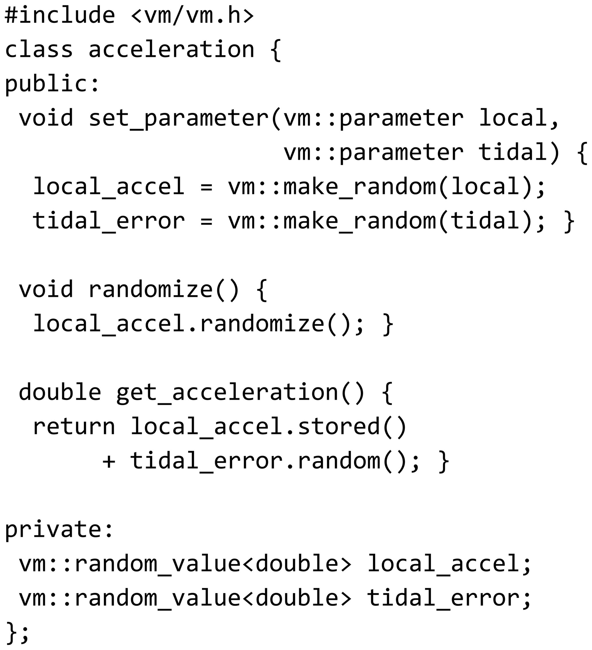
The method get_acceleration() computes and returns the sum of the randomized local acceleration and the tidal error. On each call of this method, a new random value for the tidal error is generated by invoking tidal_error.random(). To randomize the local acceleration, a separate method (conveniently named randomize()) is provided. It will be retrieved before the simulation of each measurement series begins and therefore makes the local acceleration act as a systematic effect.

It should be noted that the described model about the local gravity is only a sub-component of the very complex Planck-Balance. It was chosen for its simplicity, and therefore it is adequate for explaining the library without losing the overview. Sophisticated models can be built following the same approach.

7 Conclusions

With the aim of decreasing the effort required to set up and develop new software for uncertainty estimation, the VCMM was analyzed and generalized. As a result, a software structure was derived which can be used to guide the new developments. The reusable components of the VCMM were identified, extended, and deployed as a stand-alone software library.

The library provides many functionalities via which users can set up a general structure for an MC simulation and develop project-specific modules. Beyond the components contained by the VCMM, the library provides additional tools that address topics that are not of critical importance but are of great practical interest such as parallelization and sensitivity analysis.

The library was designed to fulfill the specific requirements of software for uncertainty estimation. However, the RNGs provided were intentionally developed in a general form to allow them to be used flexibly. Thus, it may be possible to apply some parts of the library to fields other than metrology.

The lightweight version of the VCMM was initially designed to allow its principles to be better understood. The further development of this software will contribute positively to the development of the VCMM itself.

In addition to its software, the VCMM introduces two modeling concepts. The first is the briefly described concept of so-called timescale separation, where random and systematic effects can be considered correctly by the simulation. The second concept concerns the simulation being performed based on the data from a real measurement. These two concepts are of special interest, as they may strongly impact the uncertainties resulting from the simulation. Due to their complexity, a separate discussion is required.

The development of Planck-Balance is still in progress. Therefore, the development of the VPB is also steadily continued. At the current development stage, special attention must be given to designing the software in the most general and extendable way. The next goal is to realize an uncertainty estimation that will sufficiently replicate the behavior of the real balance. With the progressing development of the PB itself, new models will be added to the VPB. Inversely, the VPB will be used to accelerate the development of the PB. In the future, the VPB is to be used for uncertainty estimations in industrial and research applications in a way comparable to how the VCMM is used today.