the Creative Commons Attribution 4.0 License.
the Creative Commons Attribution 4.0 License.
 | 29 Mar 2022
A modular adaptive residual generator for a diagnostic system that detects sensor faults on engine test beds
Michael Wohlthan
Gerhard Pirker
Andreas Wimmer
It is a great challenge to apply a diagnostic system for sensor fault detection to engine test beds. The main problem is that such test beds involve frequent configuration changes or a change in the entire test engine. Therefore, the diagnostic system must be highly adaptable to different types of test engines. This paper presents a diagnostic method consisting of the following steps: residual generation, fault detection and fault isolation. As adaptability can be achieved with residual generation, the focus is on this step. The modular toolbox-based approach combines physics-based and data-driven modeling concepts and, thus, enables highly flexible application to various types of engine test beds. Adaptability and fault detection quality are validated using measurement data from a single-cylinder research engine and a multicylinder diesel engine.
- Article
(485 KB) - Full-text XML
- BibTeX
- EndNote


Experimental investigations on engine test benches are a significant cost factor in current combustion engine development. To keep the number of required tests and their associated costs to a minimum, it is essential that sensor faults and measurement errors are detected at an early stage (Flohr, 2005). There are estimations (Fritz, 2008) that up to 40 % of test bed time is lost due to faults that are detected too late. Because of the increasing number of sensors and actuators in combustion engines, reliable validation of test results by one person alone has become nearly impossible. On the whole, there is a need for an automated diagnostic system that evaluates measurement data quality and identifies faulty measurement sensors.
A large number of diagnostic solutions exist for specific engine types, such as diesel engines (Kimmich et al., 2005; Schwarte et al., 2002) and spark-ignited automotive engines (Gagliardi et al., 2018; Svärd et al., 2013), or for subcomponents, such as the common rail system (Clever and Isermann, 2010). As these methods were expressly developed for certain engine types and, thus, for certain fault types, they are not suitable for general application on engine test beds. The great challenge in applying a diagnostic system on engine test beds is that they are often subject to frequent changes in the test engine. Therefore, the diagnostic system must be able to be adapted easily to different types of test engines. Nowadays, model-based methods using physics-based models are still common (Sarotte et al., 2020). When they are combined with data-driven techniques, hybrid procedures are obtained (Jung, 2019). This paper also follows the approach of combining physical and data-driven methods to provide models and, subsequently, residuals for fault diagnosis. Concrete methods for model generation and a complete set of physics-based models for engine test beds are presented in the paper. In addition, it is shown how the presented methods and models can be combined in a modular way in order to be used on different test engines.
The rest of this paper is organized a follows: Sect. 2 provides a short overview of the general diagnostic methodology; subsequently, a comprehensive model library is presented in Sect. 3, and a method for data-driven modeling is discussed in Sect. 4; finally, the application of the methodology is explained and evaluated using two examples in Sect. 5.
The proposed diagnostic system works according to the procedure shown in Fig. 1. The test bed produces measurement data which are combined to a measurement vector . This vector is then analyzed and checked by the three-step diagnostic procedure: residual generation, fault detection and fault isolation. In the residual generation step, a set of residuals, , is obtained from a set of models. In the fault detection step, the residuals are analyzed to determine whether a sensor fault is present in the respective measurement. Finally, in the fault isolation step, it is determined which sensors are faulty by calculating fault probabilities for all the measured variables.

2.1 Residual generation
Models for residual generation can be classified according to the type of model approach. A basic distinction can be made between physics-based models and data-driven models. Physics-based models are based purely on physical laws. Both the model structure and all model parameters are known. For data-driven models only input and output variables are considered. The internal relations are described with general mathematical formulations, and the models are generated online on the basis of previous measurements. It is assumed that both of these model types ultimately result in a quantitative model as a static relation of two general functions, f(x) and g(x), that describe the fault-free system behavior. Such a model can be formulated either as an equation
or as an inequality
In both cases, a residual r is defined as the difference between the terms before and after the operator:
As can be seen in Fig. 1, the procedure presented in this paper combines different possibilities or tools for residual generation. In this context, a tool is understood to be a user-oriented method or set of functions whose purpose is to create models for residual generation. The procedure includes the following tools:
-
The formula tool is a direct way to define a model in equation form Eq. (1) or in inequality form Eq. (2). For example, it can be used to define redundancies or simple greater than/less than comparisons, allowing the user to quickly contribute expert knowledge.
-
The limit check tool delivers two inequalities (ll<x and x<lu) per measured variable to the residual set by using a lower limit ll and an upper limit lu.
-
The model library tool provides engine-specific models. These models are grouped into component-specific modules (engine, cylinder, turbocharger, throttle valve, pipe) and include models in equation form and inequality form.
-
The data-driven modeling tool uses online model training with a continuous update of the model parameters to generate regression models that represent the correlations of the measured variables. Each measured variable is modeled as a function of all other measured variables.
Such a toolbox system is very useful for changeable systems, such as engine test beds in the field of research and development; it enables rapid adaptation of the residual set to changes in the test engine or test bed by exchanging, adding or removing individual modules, formulas, limit values or models.
2.2 Fault detection
Fault detection is performed in order to determine whether a fault has occurred or not. This is done by checking fault conditions.
Combining Eq. (3) with Eq. (1) gives
for models in equation form, and combining Eq. (3) with Eq. (2) gives
for models in inequality form.
Due to random and systematic measurement errors as well as model errors, Eqs. (4) and (5) are not directly suitable as fault conditions. In practice, it is necessary to introduce a threshold value t that takes these factors into account (Wohlthan et al., 2020), yielding the fault condition
for models in equation form and the fault condition
for models in inequality form. These two conditions describe the fault-free case. Thus, a fault is detected if one of these conditions is not fulfilled.
2.3 Fault isolation
In the case of a detected fault, a third and final step calculates fault probabilities , producing a value between 0 % and 100 % for all considered measured variables . Fault probabilities are used to identify faulty sensors, whereby the following applies: the higher the fault probability, the more likely it is that the values coming from this particular sensor are faulty and, thus, serve (the user) as important information for troubleshooting. A geometrical classification method based on the distance evaluation between error propagation curves and residual state points (Wohlthan et al., 2020) is used for this purpose. As the focus of this paper is on the residual generation and fault detection steps, the fault isolation method will no longer be discussed in this paper.
As mentioned in Sect. 2, a model library was developed for the diagnostic system presented in this paper that provides residuals for engine test bed application in modules. A module contains physics-based models and residuals representing a certain hardware component. As can be seen in Fig. 2, it is necessary to configure these modules by linking the predefined input variables to the measured variables (ui=xj).
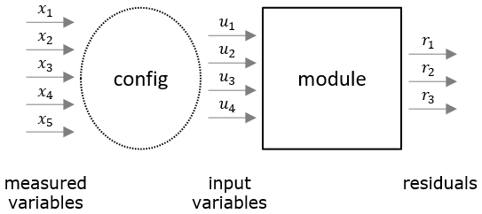
The model library presented here contains modules for the engine, cylinder, turbocharger, throttle valve and pipe. All models are listed in Table 1. While the complete model is given for simple physical relations, only the rough model structure with the necessary input variables is given for complex physical relations.
(Pischinger et al., 2009)(Pischinger et al., 2009)(Wohlthan, 2019)(Wohlthan, 2019)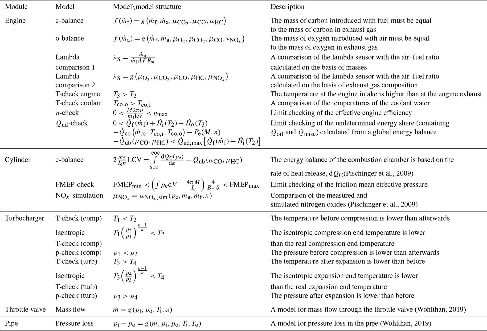
The engine module contains global relations that cannot be assigned to any specific system component but that generally apply to internal combustion engines, for example, the mass balances for carbon and oxygen or global energy considerations. The air ratio is also a central variable in the internal combustion engine, and the different possibilities for its determination provide further models.
The cylinder module uses cylinder pressure (pc) as the central measured variable and performs a thermodynamic analysis of the combustion chamber, yielding results such as the heat release rate (dQC) or a predicted value for the nitrogen oxides formed (). These results are then linked to other measured variables, thereby providing further residuals.
The turbocharger module compares input and output temperatures of the turbine and the compressor in the form of inequalities.
The throttle valve module and the pipe module connect the mass flow through the element to the pressure drop across the element. The main difference is that the mass flow model of the throttle valve module takes a variable valve position into account.
As shown in Sect. 2.1, the goal of the data-driven model tool is to generate models that deliver a predicted value for each measured variable. Assuming a data set with k measured data points, each of which consists of n measured variables , this means that one of the n variables serves as the response variable y and all other variables serve as predictor variables .
One way to obtain such models is to use regression analysis (Schadler and Stadlober, 2019). All k observations of the response variable are combined into the response vector .
All observations of each of the predictors and a column of ones for the intercept of the model are merged to the design matrix:
When using multiple linear regression,
the response is a linear combination of the predictors. The relation is disturbed by a random error , and the unknown parameter vector with l+1 components has to be estimated by the least squares method, which yields the estimate
The result is a model that represents the relation in the fault-free state.
The fully defined model is then used to predict the value of a new incoming measured data point
Finally, the difference between the predicted value and the measured value yields the residual
As can be seen above, in the prediction at a time step k+1, the data of the time steps 1 to k are used to estimate the parameters, which means that the model parameters are updated at every time step. Continuous model training is necessary for tests on engine test beds, as (due to frequently changing engine configurations) the behavior of the engine is not known in advance and can only be determined during the test. Once all necessary variations have been recorded, testing is often completed, and the test engine is changed or reconfigured.
It is possible to estimate the threshold value needed for the fault condition Eq. (6) by multiplying the root-mean-square error (RMSE) by a constant factor ft:
The model fitted with the last k observations is used for the prediction.
In the case of continuous training, the problem may arise that when an unknown operating state is reached, the residual increases sharply for a short time even in the fault-free state, leading to the fulfillment of the fault condition Eq. (6). It must be ensured that sufficient time is provided for model training so that all models can adapt to the new operating state without triggering an alarm. This can be achieved by introducing an alarm delay. An alarm delay is employed by specifying the number of measurements that the model should wait for an existing threshold violation before an alarm is triggered.
The alarm delay (da) and the threshold factor (ft) are the two parameters of the data-driven modeling tool.
In this section, the diagnostic procedure is evaluated using data from two test engines. The first engine is a single-cylinder research engine (SCE) with 27 measured variables for diagnosis, and the second one is a multicylinder diesel engine (MCE) with 51 measured variables (Fig. 3). These two completely different engine concepts show how the four tools presented in Sect. 2.1 can be used to generate a comprehensive set of residuals and further a good fault detection rate in each case.
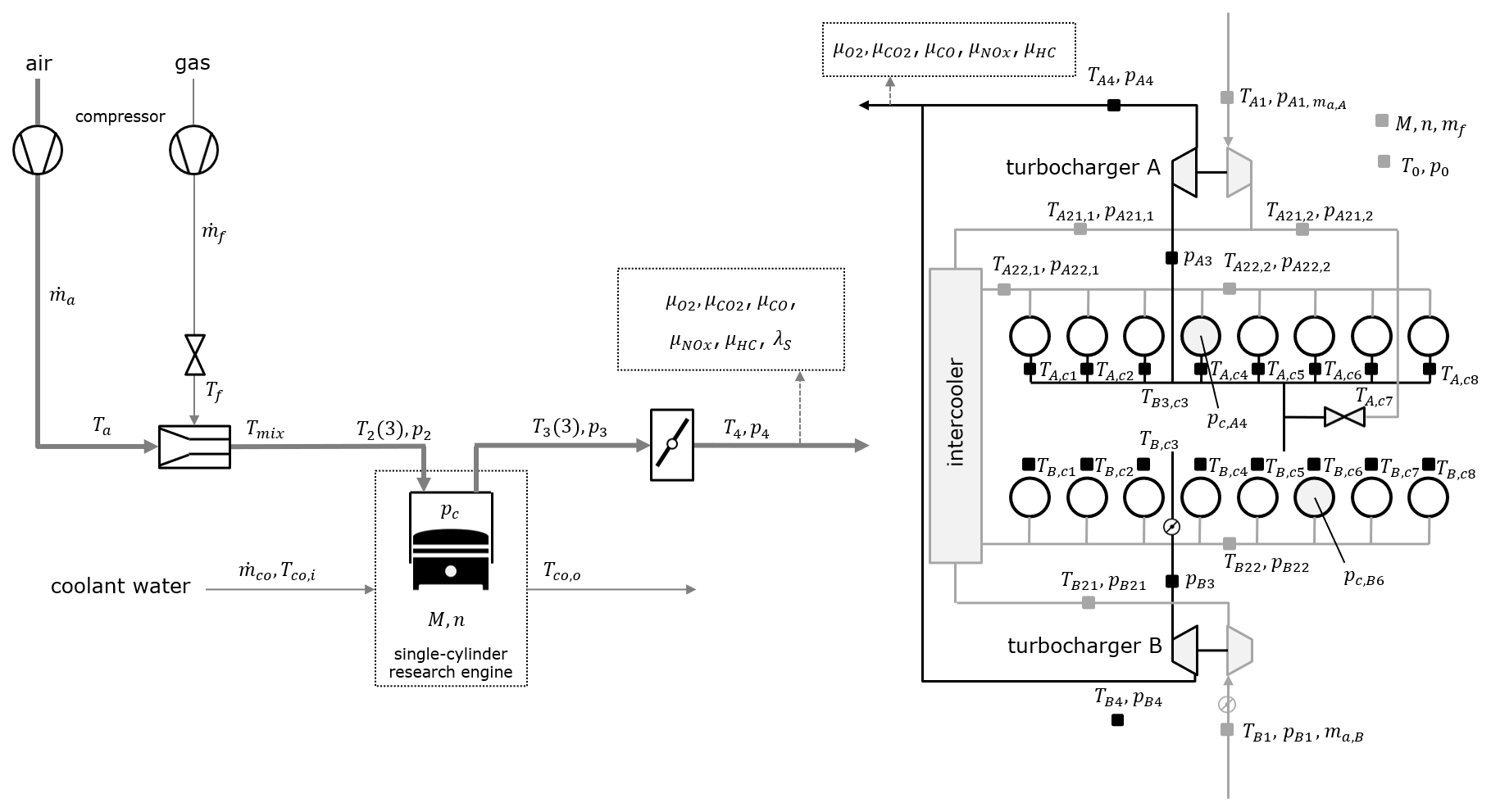
Figure 3A schematic of a single-cylinder research engine (SCE, left) and a multicylinder diesel engine (MCE, right).
5.1 Configuration of residual generation
The configuration details for each of the residual generation tools is summarized in Table 2 for both examples.
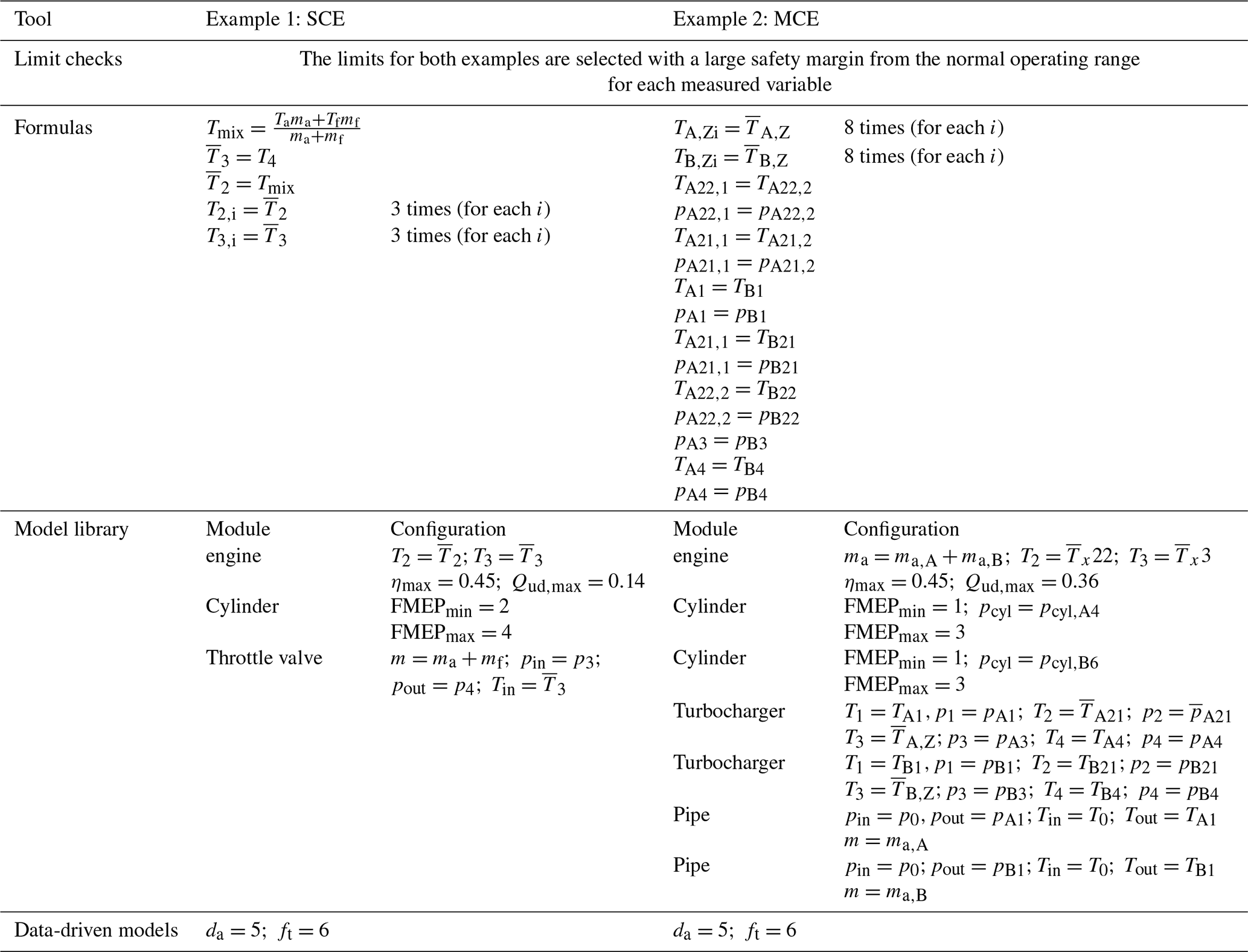
When the limits for the limit check tool were defined, care was taken to ensure a sufficient safety margin to the normal operating range of all measured variables in order to prevent false alarms in practical use. A list of the limits is not necessary beyond the current scope of this paper. The limit check tool delivers two residuals per measured variable for a total number of 54 residuals for the SCE and 102 residuals for the MCE.
The formula tool is mainly used to define pressure and temperature redundancies as well as symmetry relations resulting from the two flow paths for cylinder banks A and B in the MCE. The formula tool provides a total of 9 residuals for the SCE and 29 residuals for the MCE.
Table 2 gives an overview of the configuration of the modules used from the model library tool. The exact configuration (i.e., the assignment of a measured variable to a module input) is not specified in Table 2 if the name of the module input from Table 1 is the same as the name of the measured variable from Fig. 3. Three modules - one engine, one cylinder and one throttle valve – are used for the SCE. This results in a total number of 12 residuals (8 from the engine, 3 from the cylinder and 1 from the throttle valve). The more complex structure of the MCE requires the use of several modules. In addition to the engine module, two cylinder modules (the cylinder pressure of only two cylinders is measured) as well as one turbocharger module and one pipe module per bank are used. The “lambda comparison 1”, “lambda comparison 2” and “T-check coolant” models can not be used in the engine module, as they lack measured variables. In total, there are 29 residuals for the MCE (5 from engine, 2×3 from cylinder, 2×8 from turbocharger and 2×8 from pipe).
In both cases, the data-driven tool is operated with the default parameters and can, therefore, be operated without configuration effort. This results in a total of 27 residuals for the SCE and 51 for the MCE.
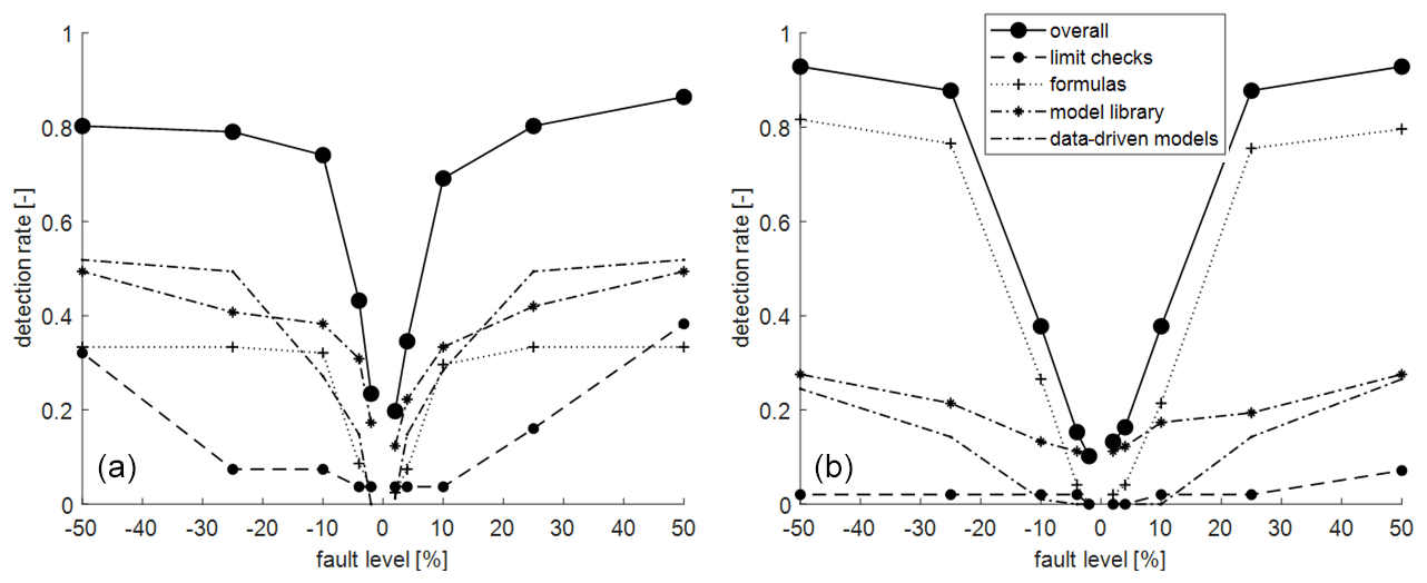
Figure 4The detection rate (RD) at specific fault levels of the individual residual generation tools for the SCE (a) and MCE (b). The detection rate at one fault level is averaged over all fault timings and variables.
5.2 Results
Fault-free measurement data from real test bed operation of these two engines provide the initial basis for the evaluation. The data set of the SCE consists of 159 data samples, and the data set of the MCE consists of 51 data samples. To evaluate the procedure, faults were simulated. The fault level, the fault timing and the affected measured variable were varied separately. A total of 10 different fault levels between −50 % and +50 % relative error were investigated. Due to the different data set size, the examined fault timings of the two examples differ. For the SCE, the fault was simulated starting with the 50th, 100th or 150th sample. The MCE, on the other hand, used either the 20th or 40th sample. In both cases, faults in all measured variables were examined. Thus, the basis for the evaluation is fault simulations for the SCE and for the MCE.
Figure 4 presents the results of the evaluation of the two examples, showing the detection rate (RD; the number of correctly detected faults divided by the number of actual faults) over the fault level of each tool and the overall result when all tools are combined. As expected, the detection rate increases as the fault level increases because threshold violations become more likely. It can be seen that the individual tools for the two examples greatly contribute to the overall result in different ways. The tools formula, model library and data-driven models deliver good results of similar magnitude for the SCE, whereas the formula tool is the main contributor to the overall MCE result due to the high number of defined formulas. Furthermore, it is apparent that the model library tool performs best at low fault levels because the physics-based models that it contains are highly accurate and, thus, generally have small model uncertainties. This leads to smaller thresholds than with the models of the formula tool and the data-driven models tool. In the case of data-driven models, the poorer performance of the MCE compared with the SCE can be explained by the fact that the quality and stability of the models is lower as a result of the smaller data set. The limit check tool is of less importance and is mainly used to detect sensor total failures and other major faults. However, good overall detection rates can be achieved in both cases, with the SCE showing better results at low fault levels because of the higher contribution of the residuals from the model library tool. The MCE, on the other hand, achieves better detection rates at higher fault levels: due to the large number of pressure and temperature variables, the influence of variables that are difficult to monitor (such as or μHC) is lower.
In this paper, it was shown how an adaptive residual generator can be realized and used for the diagnosis on engine test beds. The adaptation of the residual set to the engine or test bed is done by combining several tools and modules. As shown in the evaluation section, this system allows good monitoring of the sensors for different engine types. Depending on the application, the individual tools presented make different contributions to system monitoring. A model library consisting of component-specific modules provides the most important basis for monitoring the sensors of engine test beds. For larger data sets, the diagnostic system can be effectively supported by the use of data-driven models, which are generated automatically during the test by continuous model training. In addition, the formula tool offers the possibility to define models in equation or inequality form and add them directly to the residual set, which is especially useful for engines with a high number of redundant or quasi-redundant sensors.
| α | Throttle valve opening angle |
| η | Efficiency |
| κ | Isentropic exponent |
| λS | Lambda sensor |
| ϕ | Crank angle |
| μ | Mass fraction |
| AFRst | Stoichiometric air–fuel ratio |
| B | Cylinder bore diameter |
| C | Combustion |
| FMEP | Friction mean effective pressure |
| H | Enthalpy |
| I | Number |
| LCV | Lower calorific value |
| M | Torque |
| Pe | Effective power |
| Q | Amount of heat |
| S | Engine stroke |
| T | Temperature |
| V | Cylinder volume |
| a | Air |
| c | Cylinder |
| co | Coolant |
| eoc | End of combustion |
| ϕ | Fuel |
| i | In |
| m | Mass |
| misc | Miscellaneous |
| mix | Mixture |
| o | Out |
| p | Pressure |
| soc | Start of combustion |
| ud | Undetermined |
| ub | Unburned |
The underlying software code is proprietary and, therefore, not publicly available
The referenced data are proprietary and are owned by the project partners; therefore, they are not publicly available.
MW contributed to the conceptualization, methodology, software, validation and writing (original draft preparation). GP contributed to the conceptualization, project administration and writing (review and editing). AW was responsible for funding acquisition, project administration and supervision.
The contact author has declared that neither they nor their co-authors have any competing interests.
Publisher's note: Copernicus Publications remains neutral with regard to jurisdictional claims in published maps and institutional affiliations.
This article is part of the special issue “Sensors and Measurement Science International SMSI 2021”. It is a result of the Sensor and Measurement Science International, 3–6 May 2021.
The authors would like to acknowledge the financial support of the “COMET – Competence Centers for Excellent Technologies” program of the Austrian Federal Ministry for Transport, Innovation and Technology (BMVIT); the Austrian Federal Ministry for Digital and Economic Affairs (BMDW); and the provinces of Styria, Tyrol, and Vienna for the K1-Centre LEC 60 EvoLET. The COMET program is managed by the Austrian Research Promotion Agency (FFG).
This research has been supported by the Austrian Research Promotion Agency (grant no. 865843).
This paper was edited by Klaus-Dieter Sommer and reviewed by three anonymous referees.
Clever, S. and Isermann, R.: Modellgestützte Fehlererkennung und Diagnose für Common-Rail-Einspritzsysteme, Motortechnische Zeitschrift – MTZ, 71, 114–121, https://doi.org/10.1007/BF03225548, 2010. a
Flohr, A.: Konzept und Umsetzung einer Online-Messdatendiagnose an Motorenprüfständen, Dissertation, Technische Universität Darmstadt, Darmstadt, http://elib.tu-darmstadt.de/diss/000632 (last access: 25 March 2022), 2005. a
Fritz, S. C.: Entwicklung und Umsetzung einer zentralisierten Messdatendiagnose für Motorprüfstände als integrierter Bestandteil des Prüfstandssystems, Dissertation, Technische Universität Darmstadt, Darmstadt, https://tubiblio.ulb.tu-darmstadt.de/31088/ (last access: 25 March 2022), 2008. a
Gagliardi, G., Tedesco, F., and Casavola, A.: A LPV modeling of turbocharged spark-ignition automotive engine oriented to fault detection and isolation purposes, J. Franklin Inst., 355, 6710–6745, https://doi.org/10.1016/j.jfranklin.2018.06.038, 2018. a
Jung, D.: Engine Fault Diagnosis Combining Model-based Residuals and Data-Driven Classifiers, IFAC-PapersOnLine, 52, 285–290, https://doi.org/10.1016/j.ifacol.2019.09.046, 2019. a
Kimmich, F., Schwarte, A., and Isermann, R.: Fault detection for modern Diesel engines using signal- and process model-based methods, Control Eng. Pract., 13, 189–203, https://doi.org/10.1016/j.conengprac.2004.03.002, 2005. a
Pischinger, R., Klell, M., and Sams, T.: Thermodynamik der Verbrennungskraftmaschine, vol. 3, Springer-Verlag, Wien, https://doi.org/10.1007/978-3-211-99277-7, 2009. a, b
Sarotte, C., Marzat, J., Piet-Lahanier, H., Ordonneau, G., and Galeotta, M.: Model-based active fault-tolerant control for a cryogenic combustion test bench, Acta Astronaut., 177, 457–477, https://doi.org/10.1016/j.actaastro.2020.03.029, 2020. a
Schadler, D. and Stadlober, E.: Fault detection using online selected data and updated regression models, Measurement, 140, 437–449, https://doi.org/10.1016/j.measurement.2019.04.010, 2019. a
Schwarte, A., Kimmich, F., and Isermann, R.: Model-based fault detection and diagnosis for Diesel engines, MTZ worldwide, 63, 31–34, https://doi.org/10.1007/BF03227560, 2002. a
Svärd, C., Nyberg, M., Frisk, E., and Krysander, M.: Automotive engine FDI by application of an automated model-based and data-driven design methodology, Control Eng. Pract., 21, 455–472, https://doi.org/10.1016/j.conengprac.2012.12.006, 2013. a
Wohlthan, M.: Methoden zur Fehlerdiagnose an Motorprüfständen, Dissertation, Technische Universität Graz, Graz, https://online.tugraz.at/tug_online/pl/ui/$ctx;design=pl;header=max;lang=de/wbAbs.showThesis?pThesisNr=66703&pOrgNr=37&pPersNr=2824 (last access: 25 March 2022), 2019. a, b
Wohlthan, M., Schadler, D., Pirker, G., and Wimmer, A.: A multi-stage geometric approach for sensor fault isolation on engine test beds, Measurement, 168, 437–449, https://doi.org/10.1016/j.measurement.2020.108313, 2020. a, b
- Abstract
- Introduction
- Methodology
- Library for engine test beds
- Data-driven models
- Application examples and evaluation
- Conclusions
- Appendix A: Nomenclature
- Code availability
- Data availability
- Author contributions
- Competing interests
- Disclaimer
- Special issue statement
- Acknowledgements
- Financial support
- Review statement
- References