Gauge to simultaneously determine the electrical conductivity, the Hall constant, and the Seebeck coefficient up to 800 °C

A new high temperature gauge to simultaneously determine the electrical conductivity, the Hall constant, and the Seebeck coefficient has been developed. Screen-printed heating structures on a ceramic sample holder are used to generate temperatures up to 800 ^∘C by Joule heating. The heating structures were designed using the finite element method (FEM) simulations and the temperature distribution was validated by thermal imaging. To measure the Seebeck coefficient, $\mathrm{Au}/\mathrm{Pt}$ thermocouples with different geometries were investigated and successfully integrated into the gauge. Measurements on constantan, a typical Seebeck coefficient reference material with high electrical conductivity, high charge carrier concentration, and a known Seebeck coefficient, as well as on a well-described boron-doped silicon wafer confirm the functionality of the gauge up to 800 ^∘C.

1 Introduction

The Seebeck effect describes the generation of an electrical potential difference due to an applied temperature gradient in a material. The quotient of this so-called thermoelectric voltage U_th and the temperature difference ΔT between the two contact points is the Seebeck coefficient S as follows:

$$\begin{array}{}\text{(1)}& S=U_{\mathrm{th}}/\mathrm{\Delta }T.\end{array}$$

The Seebeck coefficient is a temperature-dependent, material-specific transport parameter and is of major importance, especially in the field of semiconductors and thermoelectrics. The Seebeck coefficient is a measure for the charge carrier density (Joffe, 1958). Materials with high Seebeck coefficients are mainly used in thermoelectric generators to convert thermal energy directly into electrical energy when a temperature gradient is present (Garofalo et al., 2020; Enescu, 2019). New materials are constantly being researched in order to advance their further development (Hendricks et al., 2022). To determine the Seebeck coefficient, a sample, mostly in the form of a bar, is clamped between two separately heatable contact surfaces (see Fig. 1). By controlling the two heaters differently, a variable temperature gradient can be generated in the sample. Two thermocouples (TCs) are typically contacted on the surface of the sample. This allows the contact point temperature to be measured and the generated thermoelectric voltage to be determined directly. The Seebeck coefficient is then calculated by the temperature difference of both contact points and the measured thermoelectric voltage. However, this calculation only provides the relative Seebeck coefficient S_relative, since the thermoelectric voltage of the leads are also included. To determine the absolute Seebeck coefficient S_absolute, the relative Seebeck coefficient and the Seebeck coefficient of the lead S_lead has to be considered as follows:

$$\begin{array}{}\text{(2)}& S_{\mathrm{absolute}}=S_{\mathrm{lead}}-S_{\mathrm{relative}}.\end{array}$$

In order to characterize materials at different temperatures, common setups are located in, often gas-flushable, furnaces. Usually, the electrical conductivity is also measured directly in such a setup. For this purpose, a current is additionally impressed between the contact surfaces at the edge of the sample and the voltage is measured by using the thermocouple leads. Such high-temperature measurement setups for both the electrical conductivity and the Seebeck coefficient for different temperature ranges are already commercially available (up to 1000 ^∘C: Advance Riko Inc., 2022; up to 1100 ^∘C: Netzsch-Gerätebau GmbH, 2022; and up to 1500 ^∘C: Linseis Thermal Analysis, 2022).

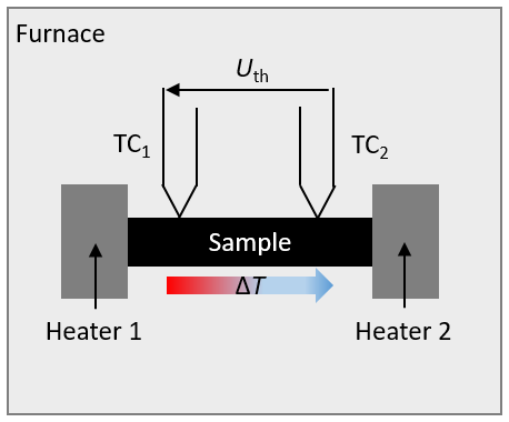
Figure 1 Representation of a typical arrangement to determine the Seebeck coefficient with a sample clamped between two heaters and two thermocouples (TC₁ and TC₂) to measure the contact point temperature and the thermovoltage U_th. Usually, such setups are installed in furnaces, if the Seebeck coefficient of the sample is to be determined at high temperatures.

However, several research groups are reporting on their own developed gauges for their individual applications (e.g., de Boor et al., 2013; Iwanaga et al., 2011). The setups published in the literature also follow a similar principle and are not considered further in detail.

With these gauges mentioned so far however, only the electrical conductivity and the Seebeck coefficient can be determined. Another important transport parameter in the field of electrical material characterization is the Hall constant R_H. Knowing the Hall constant, the charge carrier density can be derived directly, and in conjunction with conductivity data, the Hall mobility can be obtained (ASTM International, 2016). In contrast to these classical Hall effect measurements, the charge carrier density as derived by the thermoelectric measurements is almost unaffected by inhomogeneities of a sample, as it is typical for instance for conductive ceramics with less conductive grain boundaries (Gerthsen et al., 1972). For classical semiconductors, the relationship between the Seebeck coefficient and conductivity (or charge carrier density) can be described by the Jonker plot, with the typical shape of a pear (Jonker, 1968).

Yet no commercial gauge exists so far with which scientists are able to determine all of the mentioned parameters within one measurement setup at high temperatures. Kolb et al. (2013) published in 2013 their attempt of a measurement device that combines the electrical conductivity, the Hall constant, and the Seebeck coefficient up to 600 ^∘C. To the best of our knowledge, further publications neither from this nor from other research groups can be found.

In this work, we report on the integration of the measurement of the Seebeck coefficient into a previously developed setup for measuring the electrical conductivity and the Hall constant. With this new device, all three transport parameters can be measured in one cycle, using only one sample, thus saving time and material. Hence, data should be more comparable than measurements obtained from different instruments. In addition, we extended the maximum temperature from 600 to 800 ^∘C.

2 Conceptual design and requirements

The conceptual design in this work is based on the previous development of a setup for measuring the electrical conductivity and the Hall constant up to a temperature of 600 ^∘C (Werner et al., 2021). To explain the additional measurement of the Seebeck coefficient, it is first necessary to briefly describe the sample holder including the intended modifications. The conceptual design of the sample holder with the integrated measurement of the Seebeck coefficient can be seen in Fig. 2. Figure 2a shows the top side of the 635 µm thick Al₂O₃ sample holder with a flat sample area with a maximum diameter of 12.7 mm. In this area, any sample geometry can be contacted with the four freely movable, spring-mounted electrodes according to the van der Pauw method. The functionality to measure the Hall constant and the electrical conductivity of this concept up to 600 ^∘C has already been proven in a previous publication (Werner et al., 2021). To determine the Seebeck coefficient, two thermocouples are to be added, allowing to measure both the contact point temperature and the thermoelectric voltage occurring over the sample U_th. Here, care must be taken to ensure good electrical and thermal contact. Even small errors can significantly mislead the small Seebeck coefficients, which are only a few 10 µV K⁻¹ for metals and a few hundred µV K⁻¹ for semiconductors. Thereby, the exact positioning of the thermocouples is irrelevant, since the Seebeck coefficient is a geometry-independent parameter (Rettig and Moos, 2007).

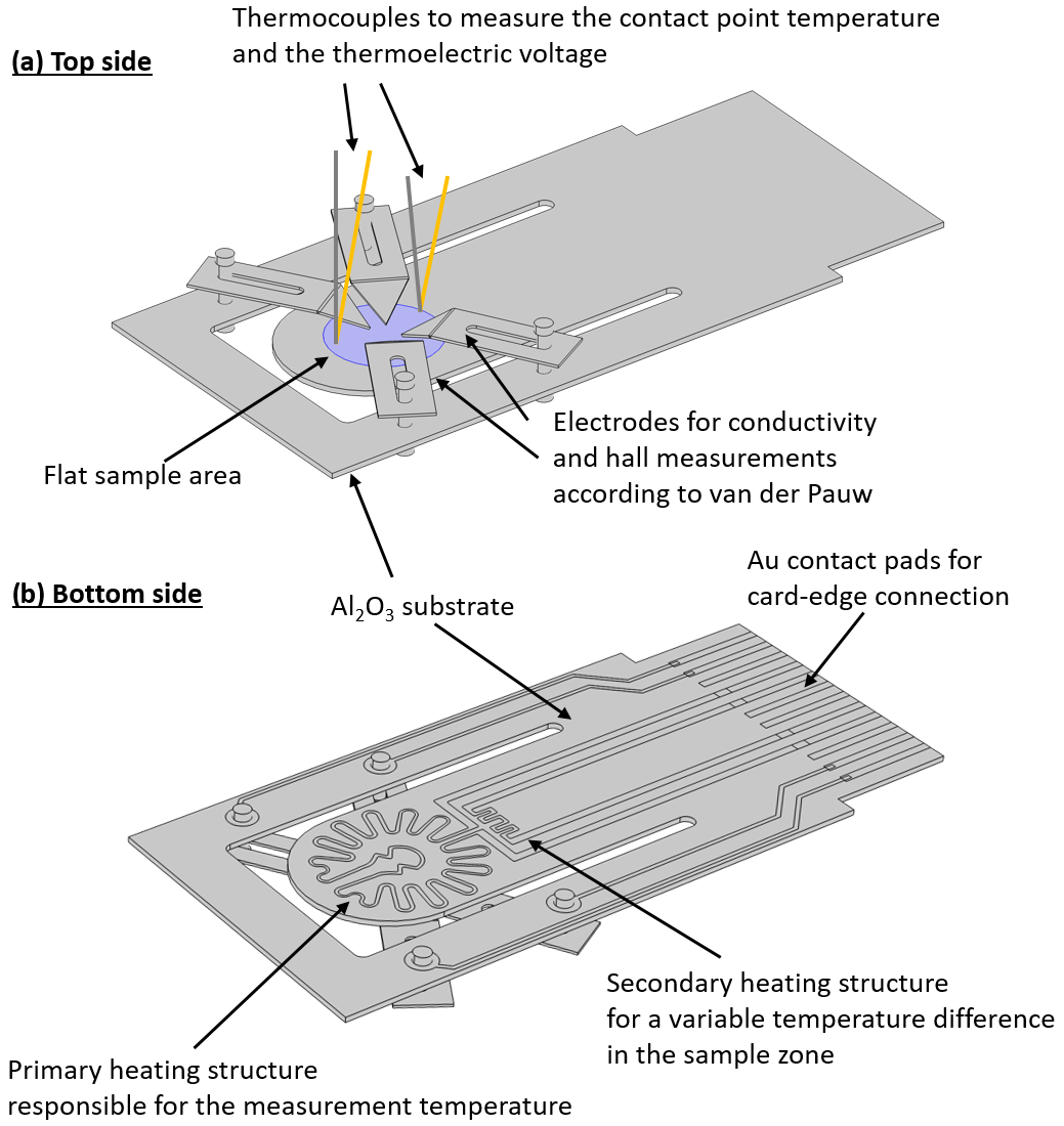
Figure 2 Sample holder concept: (a) top side of the Al₂O₃ sample holder with a flat sample zone, four movable contacts for any sample geometry according to the van der Pauw method, two additional thermocouples to measure the contact point temperature, and the thermovoltages to determine the Seebeck coefficient; and (b) bottom side of the sample holder with the primary heating structure that is responsible for the overall sample temperature and a secondary heating structure for variable temperature differences in the sample zone to determine the Seebeck coefficient.

Figure 2b shows the bottom side of the new sample holder. While in the previous work, the samples were heated by only one Pt heating structure, the new concept consists of a primary and a secondary Pt heating structure manufactured in thick-film technology. The primary heater is responsible for obtaining the maximum temperature, whereas the secondary heater works as a modulation heater allowing variable temperature differences over the sample area. For this purpose, the heating structures must be completely redesigned. Thereby, a homogeneous temperature distribution and a small variable temperature difference must be possible in the area of the sample area at any measurement temperature. In the same development step, the maximum operating temperature is to be increased to 800 ^∘C. Therefore, it is the challenge to reduce the thermally induced mechanical stresses in the substrate. They limit the maximum operating temperature to 600 ^∘C in the previous device (Werner et al., 2021). Overall, with the new measurement device, it should be possible to determine the electrical conductivity, the Hall constant, and the Seebeck coefficient in one measurement cycle up to 800 ^∘C using only one sample.

3 Development of new heating structures

In this section, the development steps of the new heating structure towards a temperature of 800 ^∘C are described. Special attention is given to the generation of both a homogeneous temperature distribution for the measurement of the electrical conductivity and the Hall constant and a variable temperature difference in the sample area for the measurement of the Seebeck coefficient. The new Pt heating structures were designed using the finite element method (FEM) simulation software COMSOL Multiphysics®, manufactured in screen-printing technology and verified using thermal imaging.

3.1 Simulation

To develop the new heating structures of the sample holder, COMSOL Multiphysics® was used. The sample holder and the heating structures were designed as shown in Fig. 3a and b. The boundary conditions of the simulation are listed in Table 1. The resistivity of the screen-printed Pt and the Al₂O₃ substrate properties were obtained from the manufacturer's data sheet.

Table 1 Simulation boundaries.

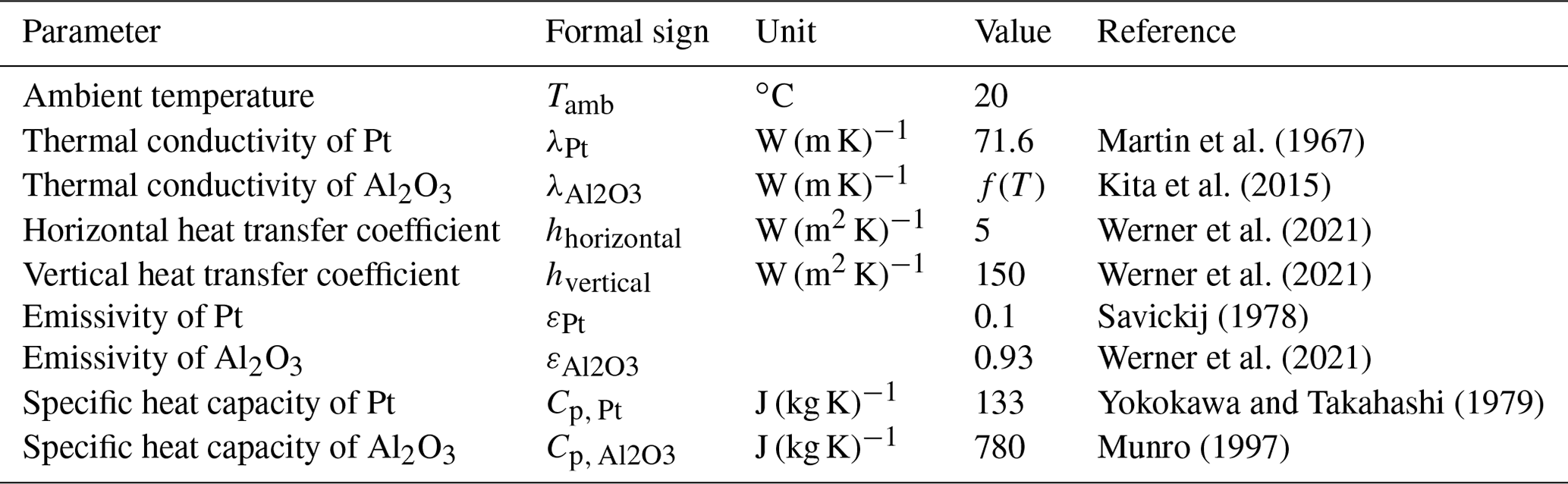
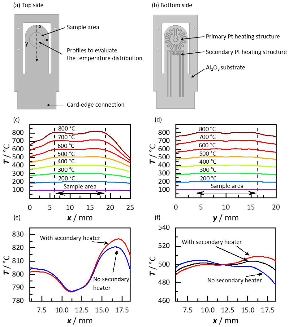
Figure 3 Simulation of the temperature distribution of the new heating structures. (a) Top view of the simulation model with sketched profiles for the evaluation, (b) bottom side of the sample holder with primary and secondary heating structure, (c) temperature profiles along the x axis at different temperatures, (d) temperature profiles along the y axis, (e) temperature profile with and without secondary heater at 800 ^∘C, and (f) temperature profile with and without secondary heater at 500 ^∘C.

Figure 3a shows the top view of the 635 µm thick Al₂O₃ sample holder. The sample area is indicated. The maximum sample area has a diameter of 12.7 mm. The temperature distribution within the sample area is evaluated on the outlined profiles along the x axis and the y axis through the center point of the sample area. The temperature profiles at different temperature steps in the steady state along the x axis are shown in Fig. 3c and along the y axis in Fig. 3d. The simulated temperature distributions along the x axis of the sample holder, i.e., along the length in the direction of the card–edge connection, show that a homogeneous temperature distribution in the sample area is possible. To ensure a homogeneous temperature distribution, the primary heater and the secondary heater are operated at the same time. The temperature difference inside the sample area at 100 ^∘C is only ±1 ^∘C, but it increases with temperature. At 500 ^∘C, the deviation within the sample zone is ±8 ^∘C. As expected, the highest temperature difference occurs at 800 ^∘C (±15 ^∘C) within the sample area of a diameter of 12.7 mm. From a percentage point of view, the deviation of the measured temperature is less than ±2 %, therefore the temperature distribution can be considered as sufficiently homogeneous in all cases. The temperature distribution in the y direction, as across the width of the sample holder, also demonstrates a homogeneous temperature distribution here (Fig. 3d). According to the simulation, measurements at homogeneous temperature distribution, i.e., especially measurements of the electrical conductivity and the Hall constant up to 800 ^∘C, are possible with the new heater design.

To measure the Seebeck coefficient, a modulated temperature difference is required. For this purpose, a negative and a positive temperature difference is intended. Thus, with the secondary heater switched off, a lower temperature should exist in the sample area in the direction of the card–edge connection, and with the secondary heater switched on, a higher temperature should be present at this position. The temperature distributions inside the sample area along the x axis (6 mm < x < 18.7 mm) without and with activated secondary heater at two exemplary temperatures are shown in Fig. 3e (800 ^∘C) and 3f (500 ^∘C). At 800 ^∘C, the temperature on the side of the card–edge connection (x≈17 mm) is already higher than the average temperature of the sample area. Nevertheless, the simulation demonstrates that with the secondary heater switched on, the temperature difference in the sample area can still be raised. Based on the results of the simulation, it can be assumed that it is feasible to determine the Seebeck coefficient at 800 ^∘C. Below 800 ^∘C, the temperature in the sample area on the side of the card–edge connection is lower than the average sample area temperature. Figure 3f illustrates three temperature profiles within the sample area at a measurement temperature of 500 ^∘C. Here, one temperature profile without the secondary heater and two others with different power of the secondary heater are demonstrated. Without a secondary heater, a temperature difference in the sample area can be observed. In this case, and respectively for all other temperature steps, the temperature on the side of the card–edge connection is slightly below the measurement temperature. By switching on the secondary heater, the temperature distribution in the sample area can be homogenized, and by increasing the heating power, the temperature difference can even be reversed. A temperature difference either between ±2 and ±10 K or 4 and 20 K is recommended for measurements of the Seebeck coefficient (Borup et al., 2015) and can be achieved at each temperature step. With the help of the simulation, two heating structures could be successfully developed. They allow homogeneous temperature distributions to measure the electrical conductivity and the Hall constant, and they allow modulable temperature differences to determine the Seebeck coefficient.

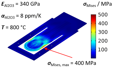
In addition to the simulations of the temperature distribution, the thermally induced stress was simulated. It has already been observed in past publications that the thermally induced stresses are usually the limiting factor for screen-printed heaters on ceramic layers (Riegel et al., 2002; Ritter et al., 2017; Werner et al., 2021). The thermally induced mechanical stress can be described by Eq. (3) as follows:

$$\begin{array}{}\text{(3)}& {\mathit{\sigma }}_{\mathrm{thermal}}=E\cdot \mathit{\alpha }\cdot \mathrm{\Delta }T,\end{array}$$

where E is the Young's modulus, α the thermal expansion coefficient, and ΔT is the temperature difference. Especially in ceramic layers with low thermal conductivity and locally limited heated areas, large temperature differences and thus high thermally induced mechanical stresses may occur. Figure 4 demonstrates the von Mises stress in the sample holder at a constant temperature of 800 ^∘C. The maximum stress occurring in the sample holder is 400 MPa. The position and the magnitude of the maximum stress are comparable to the previous generation of sample holder, but now the maximum temperature of this work is at 800 ^∘C instead of 600 ^∘C. According to the manufacturer, the maximum bending stress is 500 MPa, which suggests that a maximum operating temperature of 800 ^∘C seems achievable with the new heating structures.

Figure 4 FEM simulation of the thermally induced mechanical stress at 800 ^∘C.

3.2 Thermal imaging

To validate the new heating structures, the sample holder was produced using screen-printing technology. The heating structures made of platinum (LPA 88-11S, Heraeus, Germany) were printed directly onto the cut-to-size Al₂O₃ substrate (Rubalit 708 HP, CeramTec, Germany) and fired at 950 ^∘C. To investigate the temperature distribution, the sample holder was positioned horizontally and the heaters were connected to two external DC voltage sources. With the aid of a thermal imaging camera (VarioCAM HD, InfraTec, Germany) that was focused to the top side of the sample holder, the temperature distribution was recorded. The results are shown in Fig. 5.

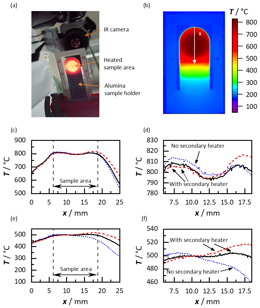
Figure 5 Thermal imaging of the sample holder. (a) Glowing sample area at 800 ^∘C (seen from the bottom side), (b) thermal image at 800 ^∘C with the profile along the x axis for the evaluation of the temperature distribution (topside view), (c) temperature distribution at 800 ^∘C along the x axis (topside view), (d) close view of the temperature distribution within the sample area along the x axis at 800 ^∘C, (e) temperature distribution at 800 ^∘C along the x axis, and (f) close view of the temperature distribution within the sample area along the x axis at 500 ^∘C.

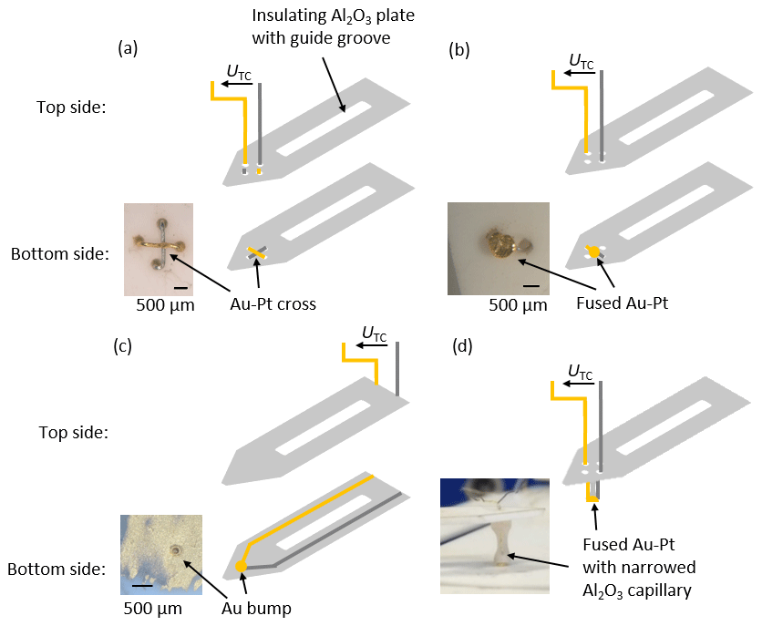
Figure 6 Schematic representation of different Au–Pt thermocouple geometries. (a) Au–Pt cross, (b) fused Au–Pt, (c) Au bump and screen-printed Au–Pt thermocouple, and (d) molten Au–Pt thermocouple with additionally narrowed Al₂O₃ capillary.

In Fig. 5a, a picture of the measurement setup can be seen from the bottom side of the sample holder with a red glowing sample area and the IR camera in the background. It is focused on the top side of the sample holder to measure the surface temperature. Figure 5b represents the temperature distribution on the top side of the sample holder at 800 ^∘C, including the drawn profile along the x axis through the center of the sample area. It is used to evaluate the homogeneity of the temperature distribution in the sample area. The first view of the temperature distribution of the sample zone on the sample holder suggests that homogeneous temperature distributions, even at 800 ^∘C, seem possible with the new heating structures. Furthermore, in Fig. 5c–f the temperature distributions along the x axis through the center of the sample zone for the exemplary temperatures of 500 and 800 ^∘C are plotted. Figure 5c shows the temperature profiles along the x axis with the highlighted sample area (6 mm < x < 18.7 mm). Figure 5d is a closer view of the sample area at 800 ^∘C with three different levels of heating power of the secondary heater. The blue dotted line denotes the temperature profile with a deactivated secondary heater. In contrast to the simulation, the temperature on the side of the card–edge connection (x=17.5 mm) is below the measurement temperature. The black drawn line illustrates the temperature profile with the activated secondary heater. The temperature distribution can be homogenized to ±8 ^∘C in the sample area. Using higher power for the secondary heater, the temperature difference in the sample area can be reversed (red dashed line). The temperatures derived with the IR camera at 800 ^∘C differ only slightly from the simulated ones but exceed expectations in this respect. The small differences between simulation and measurement can be explained by the boundary conditions of the simulation. For example, the heat flow in the direction of the card–edge connection seems to be somewhat larger in reality than assumed. Nevertheless, the measurements demonstrate that a very homogeneous temperature distribution and positive and negative temperature differences for Seebeck coefficient measurements can be achieved, even at 800 ^∘C. In addition, IR images were also taken at 500 ^∘C. The results are plotted in Fig. 5e and f. As already seen for 800 ^∘C, the temperature profile along the x axis drops in the direction of the card–edge connection when the secondary heater is inactive (blue dotted line). By activating the secondary heater, the temperature distribution can be homogenized to 500 ^∘C ± 2 % (black drawn line). Again, by increasing the power of the secondary heater, the temperature difference can be reversed, enabling to measure the Seebeck coefficient with positive and negative temperature differences (red dashed line).

All in all, the IR camera measurements validate the simulations and thus also confirm that with the new heating structures can the measurements be carried out up to 800 ^∘C. Both a homogeneous temperature distribution (measurement of the electrical conductivity and the Hall constant) and a variable temperature difference (measurements of the Seebeck coefficient) are possible with the new sample holder generation.

4 Development of suitable thermocouples

The Seebeck coefficient of metals is in the range of a few µV K⁻¹ and for semiconductors in the range of a few hundred µV K⁻¹. Therefore, even small errors, whether in the measurement of the small thermovoltages or in the contact point temperatures, may lead to erroneous results. For this reason, suitable thermocouple materials and geometries will be discussed in this section, to counteract these error sources.

4.1 Material selection

Since this work is an extension of an existing measurement setup, the geometric boundary conditions cannot be modified, despite having a significant influence on the material selection of the thermocouples. The sample holder will be installed into a measurement chamber with an overall height of only 15.5 mm. From the top side of the sample holder to the wall of the measurement chamber therefore, only about 7 mm are available to install the thermocouples, which is why the thermocouples must be flexible, at least to certain degree. Furthermore, the calculation of the Seebeck coefficient requires precise knowledge of the contact point temperatures. Therefore, the thermocouples should have an appropriate sensitivity between room temperature and 800 ^∘C. For applications at higher temperatures in different gas atmospheres, they should also be resistant to oxidation and reduction. Suitable material combinations could be NiCr–Ni (type K), PtRh–Pt (type S), and Au–Pt thermocouples. Type S and type K are the most common used thermocouples and are generally sold sheathed. In this case, the two thermocouple wires are embedded in ceramic and covered with a metallic sheath. This has two disadvantages for the here-intended application. On the one hand, the ceramic filling reduces the flexibility of the thermocouples and, on the other hand, the measurement point of the temperature is not the electrical contact point with the sample surface. This leads to a temperature error. For this reason, sheathed thermocouples were not used. However, type K and type S thermocouples can also be used as wire-only thermocouples. With about 41 µV K⁻¹, the type K thermocouple has the highest sensitivity of all the materials mentioned (Park et al., 1993). Nevertheless, type K thermocouples oxidize above 800 ^∘C, resulting in drift and decalibration. Furthermore, the hysteresis between 300 and 600 ^∘C can lead to measurement errors of several degrees (Childs et al., 2000).

Type S thermocouples, on the contrary, are not expected to oxidize (Ripple and Burns, 1998). Unfortunately, the sensitivity is only about 5–10 µV K⁻¹ between room temperature and 800 ^∘C. This may lead to temperature measurement errors due to unprecise thermoelectric voltage measurements of the thermocouple.

Another possibility is to apply Au–Pt wires as thermocouples. This combination is not widely used, but has higher sensitivity than type S thermocouples (Kim et al., 1998). The temperature-dependent thermoelectric voltage of Au–Pt thermocouples is documented in literature (Gotoh et al., 1991). The polynomial characteristics relative to a reference temperature of 0 ^∘C varies between 128.2 µV at room temperature and 12.289 mV at 800 ^∘C, which corresponds to a sensitivity of ≈9–21 µV K⁻¹. Another advantage is the oxidation and reduction resistance of the noble metal. Moreover, Au and Pt wires are available in different diameters, allowing to customize the design, especially if space is limited. Thermocouples made of Au–Pt seem to be suitable for this measurement setup. Hence, only Au–Pt thermocouples will be discussed in the following.

4.2 Thermocouple geometry

When measuring the surface temperature with thermocouples, three sources of errors may occur that are to be minimized during the preliminary tests. The probably largest error stems from the influence of the thermocouple to the surface temperature itself. Contact with the surface disturbs the temperature field, and the heat flow through the thermocouple reduces the temperature at the contact point. This error can only be reduced but not prevented. Another source of error is the thermal contact resistance of the contact surfaces between the thermocouple and the sample. The geometric offset of the thermocouple measuring point from the actual measuring point on the surface can be considered the third source for errors (Bernhard, 2014). In order to investigate these error sources experimentally, four thermocouple geometries were manufactured. The Inconel electrodes of the previous setup (see Werner et al., 2021) were replaced by thin electrically insulating, but less thermally conductive, Al₂O₃ platelets with a recess. The thermocouples were made out of Au (Au 4N, Agosi, Germany) and Pt (99.99 %, Agosi, Germany) wires, each with a diameter of 100 µm. The different thermocouple geometries are depicted in Fig. 6.

For the first thermocouple, four 200 µm diameter holes in a square arrangement were laser cut at the tip of the 635 µm thick Al₂O₃ platelets. The Au and Pt wires were passed through the holes and arranged in a cross on the bottom side (see Fig. 6a). The Al₂O₃ platelets can be pressed onto the sample holder surface with the Au–Pt cross. This causes a contact between the two thermocouple wires, and thus the temperature measurement point is also created. In this case, it is important to use thin wires to minimize the distance from the temperature measuring point to the contact point. In addition, the arrangement of the wires plays an important role. The gold wire should be in contact with the sample, since on the one hand it is softer and thus adapts better to the surface properties of the sample, thus reducing the thermal contact resistance, and on the other hand gold has a significantly higher thermal conductivity (λ_Au = 310 W (m K)⁻¹) than platinum (λ_Pt = 71.6 W (m K)⁻¹), thus reducing the error due to the distance between the measuring point and the electrical contact point with the sample surface.

Another embodiment of the Au–Pt thermocouple is shown in Fig. 6b. On the bottom side of the Al₂O₃ platelets, the wires are brought together and fused. When the gold wires are heated, a ball forms intrinsically due to the high surface tension (similar to gold wire bonding). This allows balls of any diameter of gold to be created, surrounding the platinum wire. To minimize thermal contact resistances, the balls were then mechanically shaped to create a contact surface with a diameter of about 500 µm. Again, the contact point and the measurement point are distant from each other, but because of the high thermal conductivity of gold, only a small measurement error is to be expected.

Another possible thermocouple geometry is illustrated in Fig. 6c. It consists of screen-printed Au and Pt on the bottom side of the Al₂O₃ platelets. The contact to the surface is realized via a 75 µm high Au bump. The Au bump was manufactured by using a manual ball wedge bonder (HB05, TPT, Germany). The use of a bonder allows very small, point-shaped contacts to be made, as required for the measurement of electrical conductivity and the Hall constant according to the van der Pauw method. With a diameter <100 µm, the contact area of the contact point is the smallest of all the shown thermocouples.

The fourth thermocouple in Fig. 6d has similarities to the previously described thermocouple of Fig. 6b. It consists of fused and mechanically deformed Au–Pt. Unlike the other thermocouples, a narrow Al₂O₃ capillary was installed between the Al₂O₃ platelets and the contact points to further decouple the sample and the Al₂O₃ platelets.

In order to investigate the influence of the different thermocouple geometries, the different thermocouples were installed on the top side of the sample holder with a screen-printed heating structure on the bottom side. The setup is depicted in Fig. 7a. On the surface of the top side, a fixed position in the sample area was defined. The temperature at this point was determined by thermal imaging with an IR camera. During the experiment, each thermocouple was positioned there, ensuring the direct comparability of the results. The sample holder was heated in 100 ^∘C steps between 100 and 500 ^∘C, and the thermovoltage of the respective thermocouples were measured by a Keithley 2700 digital multimeter. After each measurement cycle, the thermocouple was exchanged and the measurement was repeated. In Figure 7b, the thermocouple voltage over the previously calibrated temperature at the fixed contact point are shown. The symbols denote the measured results, while the continuous lines stand for the corresponding polynomial fit functions. The voltages obtained from the Au bump thermocouple (Fig. 6c) differ most clearly from the Au–Pt characteristic. At a fixed point temperature of 500 ^∘C, a thermovoltage of only 4.29 mV was measured, whereas 6.3 mV would have been expected. The voltage corresponds to a temperature of only ≈380 ^∘C. Less deviations occur with the Au–Pt cross thermocouple (Fig. 6a). At 500 ^∘C, the thermovoltage is only 1.05 mV below the expected one, resulting in a temperature of 440 ^∘C. With the fused Au–Pt thermocouple (Fig. 6b), the measured temperature is only slightly higher. The best agreement with the expected curve can be achieved with the fused thermocouple with a narrowed Al₂O₃ capillary (Fig. 6d). The measured thermovoltage is ca. 300 µV below the characteristic curve, which corresponds to a temperature difference of only 9 ^∘C at a fixed point temperature of 500 ^∘C.

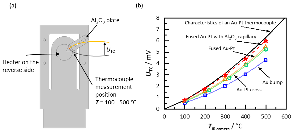
Figure 7 Measurements with the different Au–Pt thermocouple geometries: (a) schematic representation of the setup with a sample holder with integrated heating structure on the bottom side and a fixed thermocouple measurement position, and (b) thermovoltages as obtained by the different thermocouple geometries (see Fig. 6) compared with the Au–Pt characteristics from Gotoh et al. (1991).

One may explain the differences between the measured thermovoltages (and hence temperatures) and the expected ones when considering the analogy of current and voltage with heat flow and temperature difference. The thermal resistance of a heat conductor is calculated from its length l, its cross-section A, and its thermal conductivity λ, according to Eq. (4). In analogy to Ohm's law, the temperature difference ΔT is calculated from the product of the thermal resistance R_th and the heat flow $\dot{Q}$ (Eq. 5). Furthermore, the analogous laws of series and parallel circuits also apply in thermodynamics. Thus, the heat flow of a series circuit is limited by the largest thermal resistance of a system.

$$\begin{array}{}\text{(4)}& {\displaystyle }{R}_{\mathrm{th}}={\displaystyle \frac{l}{\mathit{\lambda }A}}\text{(5)}& {\displaystyle }{R}_{\mathrm{th}}\cdot \dot{Q}=\mathrm{\Delta }T.\end{array}$$

The Al₂O₃ platelets with the integrated thermocouples and the contact resistances can all be considered as a series connection of different thermal resistors. In case of the Au bump thermocouple, the Au bump seems to have the highest thermal resistance and limits the heat flow, due to its small geometry. According to Eq. (5), the high thermal resistance at the Au bump leads to a large temperature difference ΔT between the nominal and the actual temperatures from Fig. 7b. In comparison, the thermal resistances of the cross and the fused thermocouples are lower, which is why lower temperatures differences are found at this point. The significantly better results of the fourth thermocouple (Fig. 6d) can be attributed to the Al₂O₃ capillary. The narrowed Al₂O₃ capillary adds another thermal resistor to the system, which is now the highest and limits the heat flow. Due to the generally lower heat flow, the temperature drop at the thermocouple is lower, resulting in a higher measurement temperature.

The measurements and also the theoretical consideration show that in order to derive the contact point temperature precisely, not only the thermocouple geometry but also the entire geometry of the contacts affect the heat flow and the measured temperature to a large extent. Therefore, it is recommended to reduce the heat flow $\dot{Q}$ to the outside (so-called “cold-finger effect” (Edler and Huang, 2020)) by a bottleneck and to keep the thermal resistance R_th of the thermocouple itself as low as possible. According to Eq. (5), the temperature difference ΔT at the thermocouple will then be as small as possible.

5 The sample holder

After developing the new heating structures and the selection of suitable thermocouples including their geometries, the new sample holder generation was manufactured.

It is shown in Fig. 8. It consists of a 635 µm thick Al₂O₃ substrate with screen-printed heating structures on the bottom side. The two heating structures were additionally covered with another electrically insulating layer (QM42, DuPont). Furthermore, a Pt temperature sensor in four-wire technique was integrated on the bottom side, to be able to determine the temperature in the sample area after one-time calibration. The 12.7 mm diameter sample area is located on the top side. The contacts for the measurements of the van der Pauw measuring method are still realized by four spring-mounted freely movable Inconel contacts. As investigated and discussed in the section before, the fused Au–Pt thermocouples were integrated in this setup. Instead of a narrowed Al₂O₃ capillary, the heat flow to the outside is limited by the tip of the mechanically deformed Inconel contacts. The thermocouples with a contact surface of about 500 µm in diameter can easily be clamped between the Inconel contacts and the sample to measure the contact point temperatures. The thermocouple wires are routed separately from the sample holder and can be connected to a Keithley 2700 digital multimeter in the cold area under consideration of the reference junction temperature. The thermovoltage is measured between the Pt leads of the thermocouples. All other connections to the electronics are made via a card–edge connection. Here, the primary and secondary heaters are connected to two separate external power supplies and are controlled independently. The four-wire resistance of the temperature sensor on the bottom side is measured using a Keithley 2700 digital multimeter. A Keithley 2400 SourceMeter is used to impress a DC current during the electrical conductivity and the Hall constant measurements. The low voltages during measurements are recorded via a Keithley 2182A Nanovoltmeter. An additional relay circuit was programmed, to automatically switch the contacts during measurement, in accordance with the international standard ASTM F76-08 (ASTM International, 2016).

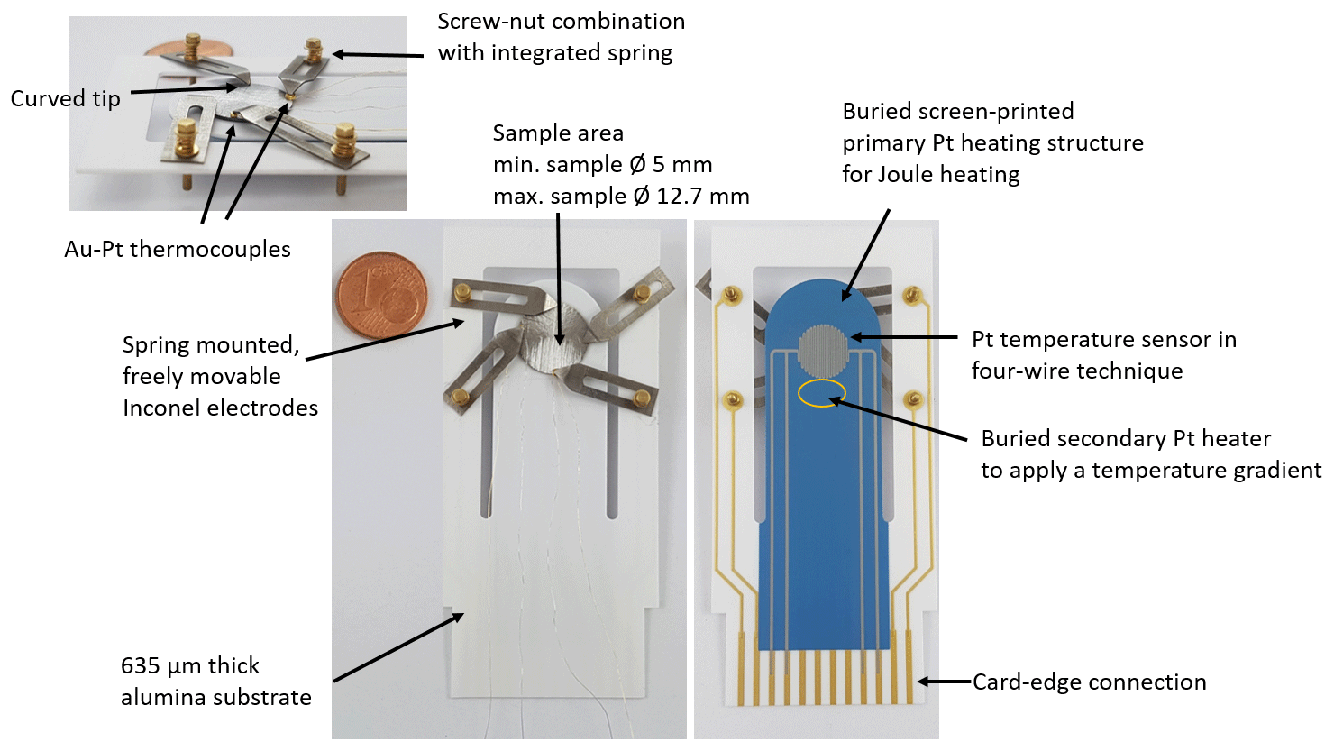
Figure 8 New sample holder generation with screen-printed primary and secondary heater, additional Pt temperature sensor, four freely movable, spring mounted electrodes, and two Au–Pt thermocouples.

Seebeck functionality test

As a first step, the setup to measure the Seebeck coefficient had to be validated. For this purpose, two different samples were measured and compared with literature data or with measurements from known established instruments. Samarium-doped calcium manganate, a typical semiconducting material that is used to manufacture high temperature thermoelectric generators (Bresch et al., 2018), and constantan, as well-known reference material (Bentley, 1998), were used. The samples were contacted with two fused thermocouples on its surface. The measured contact point temperatures were used to control the heating structures on the bottom side of the sample holder. The temperature was determined from the mean value of both thermocouple temperatures (($T_{\mathrm{TC}\mathrm{1}}+T_{\mathrm{TC}\mathrm{2}})/\mathrm{2}$). By varying the power of the secondary heater, the temperature difference was modulated. The sample holder was heated in 100 ^∘C steps up to a maximum of 700 ^∘C. As representative for all measurements, the raw data of samarium-doped calcium manganate at 600 ^∘C are plotted in Fig. 9.

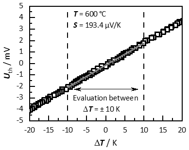
Figure 9 Raw data of a measurement of the Seebeck coefficient of samarium-doped calcium manganate at 600 ^∘C.

Figure 9 shows the thermovoltage. It was measured between the platinum leads of the thermocouples and has not yet been corrected with the thermovoltage of platinum, versus the temperature difference of the contact points. It can be clearly seen that the thermoelectric voltage increases linearly with increasing temperature difference. The data include several heating and cooling cycles without any hysteresis. Furthermore, almost no voltage offset at a temperature difference of 0 K occurs. Both are indicators of a good measurement quality (Borup et al., 2015). The Seebeck coefficient was calculated from the slope of the thermovoltage in the ΔT range of ±10 K. A larger evaluation range with temperature-dependent Seebeck coefficients would yield erroneous results (Borup et al., 2015). However, the slope of the measured thermovoltages represents only the relative Seebeck coefficient (see Eq. 1). To determine the material-specific absolute Seebeck coefficient, the Seebeck coefficient of the platinum leads, S_Pt, must be taken into account (Kockert et al., 2019). S_Pt is temperature-dependent but well documented in literature (White and Minges, 1997). For small temperature differences, the absolute Seebeck coefficient was calculated by combining Eqs. (1) and (2) with S_lead=S_Pt of the respective temperature as follows:

$$\begin{array}{}\text{(6)}& \begin{array}{rl}{S}_{\mathrm{absolute}}& \left({\displaystyle \frac{T_{\mathrm{TC}\mathrm{1}}+T_{\mathrm{TC}\mathrm{2}}}{\mathrm{2}}}\right)=S_{\mathrm{Pt}}\left({\displaystyle \frac{T_{\mathrm{TC}\mathrm{1}}+T_{\mathrm{TC}\mathrm{2}}}{\mathrm{2}}}\right)\\ & -{\displaystyle \frac{U_{\mathrm{th}}}{T_{\mathrm{TC}\mathrm{1}}-T_{\mathrm{TC}\mathrm{2}}}}.\end{array}\end{array}$$

The absolute Seebeck coefficients of constantan and of samarium-doped calcium manganate versus temperature are plotted in Fig. 10. Figure 10a shows two independently performed measurements on constantan. To evaluate the derived data, in Fig. 10a, the data for the constantan standard reference are included as well. It can be seen that the obtained Seebeck coefficients, especially up to 200 ^∘C, agree with the reference. At 300 ^∘C, the largest deviation occurs. A possible explanation for the deviation could be the surface oxidation in air atmosphere above 300 ^∘C (Brückner et al., 1995). It has to be mentioned that the reference measurements were carried out in He atmosphere, where no surface oxidation is to be expected. However, above 300 ^∘C, the measured values differ slightly from the reference, but even up to 700 ^∘C, the deviation is less than 10 %. All these deviations may occur because of the surface oxidation, but anyway, small deviations are to be expected for measurements of the Seebeck coefficient in general. Even with high-precision measurement instruments and measurements on the same materials, the deviation is generally ±5 % (Lowhorn et al., 2009). Manufacturers of existing instruments even specify a measurement accuracy of only ±7 % (Linseis Thermal Analysis, 2022; Netzsch-Gerätebau GmbH, 2022; Advance Riko Inc., 2022). Overall, the measurements on constantan confirm the functionality of the Seebeck coefficient measurement with this new sample holder generation up to 700 ^∘C. Furthermore, Fig. 10a provides an initial indication of the reproducibility of the measurement results. The series of measurements shown were carried out independently, and the sample was removed and re-installed for each series of measurements.

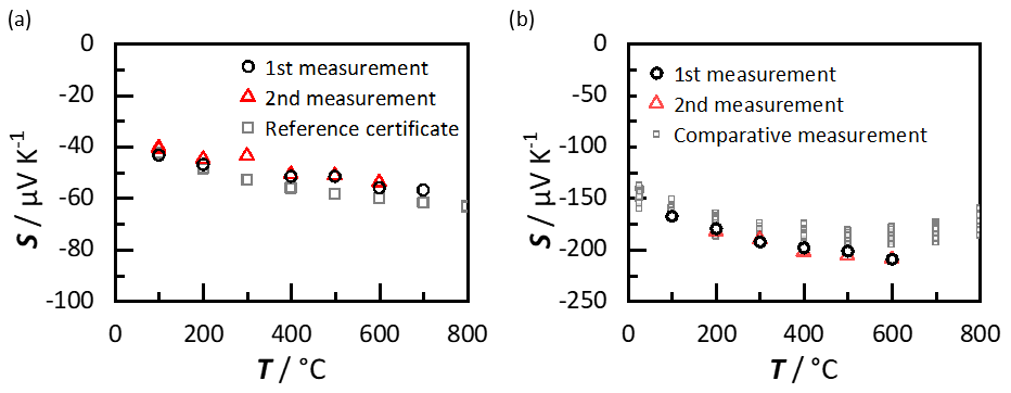
Figure 10 Measurement of the Seebeck coefficient up to 700 ^∘C: (a) Seebeck coefficient of constantan, a standard reference material; and (b) Seebeck coefficient of samarium-doped calcium manganite, a typical material for thermoelectric generators for high temperature applications.

The Seebeck coefficients of another two samples series of samarium-doped calcium manganate are shown in Fig. 10b. The measurements again are well reproducible up to 600 ^∘C and agree well with data obtained in another, already established measurement device (Bresch et al., 2018). With a deviation of less than ±10 %, the functionality of the Seebeck coefficient gauge is again verified.

Nevertheless, measurements up to 800 ^∘C have not been performed during these initial functionality tests. This is mainly due to caution of a mechanical failure due to thermally induced mechanical stresses. The measurements up to 800 ^∘C can be found in the next section.

6 Combined measurements

Having demonstrated the functionality of the Seebeck coefficient measurements in this work (and the electrical conductivity and Hall constant measurements in a previous work (Werner et al., 2021)), in this section, the combination of the three measurements in one cycle is given.

6.1 Experimental setup and procedure

The sample holder shown in Fig. 8 can be fixated horizontally in an aluminum chamber. The sample holder can then be controlled to the desired temperature with a heating rate of more than 50 K min⁻¹. The temperature should be maintained for at least 10 min to ensure a homogeneous temperature distribution along the sample holder. First, the electrical conductivity is measured according to the ASTM International Standard F76-08 (ASTM International, 2016). Subsequently, measurements in the magnetic field are carried out. For this purpose, two magnetic yoke systems consisting of permanent magnets, each with a magnetic flux density of ±760 mT, are moved across the aluminum chamber. A detailed description of the setup can be found in (Werner et al., 2021). The measurements of the Hall constant also follow the guidelines of ASTM F76-08. Finally, the Seebeck coefficients were measured in a magnetic field-free position before the next temperature is set.

6.2 Measurement results

In order to validate the combined gauge, the electrical conductivity, the Hall constant, and the Seebeck coefficient were measured within one cycle. Therefore, constantan as a typical Seebeck coefficient reference material with high electrical conductivity, high charge carrier concentration, and a known Seebeck coefficient, and a well-described boron-doped silicon wafer were measured. The constantan sample (thickness: 620 µm) had a circular shape, while the silicon wafer (thickness: 380 µm) was previously laser cut in a cloverleaf structure. The following data show the results of the combined measurements. All electrical transport parameters of each sample were obtained in one cycle and during the heating period. For a more individual discussion, the individual procedures and the results are discussed separately in the following.

6.2.1 Electrical conductivity

The electrical conductivity was measured according to the van der Pauw method (van der Pauw, 1958). Therefore, the sample was contacted via four electrodes. In samples with arbitrary geometry, like constantan in our case, the samples were contacted at the edge with contacts as small as possible. For samples in the cloverleaf structure, the contact size and position play only a minor role, provided that only one contact per cloverleaf is used. For the electrical conductivity measurement, a current was impressed between two adjacent electrodes, and the voltages were measured at the remaining two electrodes. Subsequently, the contacts were changed clockwise and also measured with opposite current polarity. From the total of eight recorded voltages and the sample thickness, the resistivity or the conductivity were then be calculated according to ASTM International (2016).

Figure 11 shows results of the electrical conductivity of constantan and the boron-doped Si wafer in the Arrhenius-like representation up to 800 ^∘C. Here, the results of constantan can be seen in black triangles and the ones for the Si wafer in red squares. In addition to the measured values, the reference values are also plotted (dashed). For constantan, the measured values were taken from a standard reference certificate from Linseis, and for silicon, the literature data were plotted in the intrinsic range of conductivity adapted from Morin and Maita (1954).

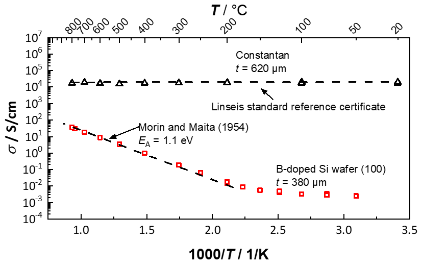
Figure 11 Arrhenius-like representation of the electrical conductivity of constantan (thickness: 620 µm) and a boron-doped Si wafer (thickness: 380 µm) up to 800 ^∘C. Both measurements agree well with the references.

The electrical conductivity of constantan was first measured at room temperature. Then the temperature was increased in 100 ^∘C steps to the maximum temperature of 800 ^∘C. It can be clearly seen that the derived conductivity of constantan agrees very well with the reference certificate. With increasing temperature, the conductivity of constantan hardly changes, which is typical for this material. The temperature coefficient of the resistance is given in the literature as only $\mathrm{10}\times {\mathrm{10}}^{-\mathrm{6}}$ K⁻¹ and confirms the minimal change in conductivity despite the high measurement temperature (Hagart-Alexander, 2010).

In contrast, the electrical conductivity of the boron-doped silicon wafer changes by several decades in this wide temperature range. At the beginning, in the range of 50–175 ^∘C, the conductivity of the silicon wafer hardly changes. According to Fasching (2005), in this temperature range, the charge carrier density remains constant (determined by the doping level). With increasing temperature above 175 ^∘C, there is a significant change in the electrical conductivity. Above 200 ^∘C, the range of intrinsic conductivity of this boron-doped Si wafer is already reached. Due to the external energy in the form of heat, electrons are transferred from the valence band to the conduction band, forming an electron–hole pair, which is why both types of charge carriers contribute to the electronic conduction in this temperature region. For comparison with literature, the dashed line plots the measured values of Morin and Maita (1954). The measured electrical conductivity of the Si wafer agrees very well with the literature reference. In addition, the Arrhenius-like representation leads to a band gap of 1.1 eV, which also agrees with the literature (Kittel, 2018; Li, 1978). Both series of measurements demonstrate that it is possible to determine electrical conductivities up to 800 ^∘C with the here-shown gauge.

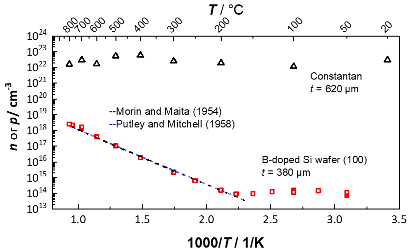
Figure 12 Arrhenius-like representation of the charge carrier densities of constantan (n) and a boron-doped Si wafer (p) up to 800 ^∘C. Additionally, the charge carrier concentration data from the intrinsic conductivity of silicon, as adapted from Morin and Maita (1954) and Putley and Mitchell (1958), are shown.

6.2.2 Hall coefficient

To measure the Hall coefficient, a current is impressed between two opposing electrodes and the voltage is measured between the remaining ones. Due to a perpendicular magnetic field and the resulting Lorentz force, a Hall voltage U_H forms (Putley, 1960). Subsequently, the contacts of current and voltage are switched, and the measurement is repeated. This procedure is also carried out with opposite polarity of the current and in a reversed magnetic field. From all these eight obtained voltages, the thickness t of the sample, the magnetic flux density B, and the impressed currents I, the Hall coefficient can be calculated according to ASTM International (2016).

Knowing the Hall coefficient and the charge carrier type, the charge carrier density can be determined. For each type of charge carrier, the charge carrier density can be calculated according to Eqs. (7) and (8), where r is a material-specific transport parameter, n and p are the charge carrier densities of the respective charge carrier type, and e is the elementary charge.

$$\begin{array}{}\text{(7)}& {\displaystyle }{R}_{\mathrm{H}}=-{\displaystyle \frac{r}{ne}}\text{(8)}& {\displaystyle }{R}_{\mathrm{H}}=+{\displaystyle \frac{r}{pe}}.\end{array}$$

For the transport parameter r, $\mathrm{3}\mathit{\pi }/\mathrm{8}$ was assumed in the case of silicon (Pearson and Bardeen, 1949) and 1 for constantan (ASTM International, 2016). However, the equations apply only in the case of one single type of charge carrier. In the case of intrinsic conduction in semiconductors, electrons and holes contribute to the conduction, so both must also be included in the calculation. The calculation requires knowledge about the ratio of the charge carrier mobility or the number of charge carriers, and it can be calculated from the Hall constant according to Eq. (9).

$$\begin{array}{}\text{(9)}& R_{\mathrm{H}}=r{\displaystyle \frac{p{\mathit{\mu }}_{\mathrm{p}}^{\mathrm{2}}-n{\mathit{\mu }}_{\mathrm{n}}^{\mathrm{2}}}{e{\left(p{\mathit{\mu }}_{\mathrm{p}}+n{\mathit{\mu }}_{\mathrm{n}}\right)}^{\mathrm{2}}}}.\end{array}$$

The temperature-dependent electron mobility μ_Hn = 4 × 10⁹ (T K⁻¹)^−2.6 cm² (V s)⁻¹ and the hole mobility μ_Hp = 2.5×10⁸ (T K⁻¹)^−2.3 cm² (V s)⁻¹ were used to calculate the charge carrier density in the intrinsic conductive region of silicon (Pfüller, 1977). The calculated charge carrier densities are shown in Fig. 12.

Constantan, as an alloy (Cu₅₄Mn₁Ni₄₅), is expected to behave in a metal-like way. The charge carrier density of constantan calculated from the measured Hall constant is $\approx \mathrm{2}\times {\mathrm{10}}^{\mathrm{22}}$ cm⁻³ and is comparable to the charge carrier density of Cu₅₅Ni₄₅ found in the literature (Köster and Schüle, 1957). Similar to metals, the charge carrier density remains constant over the wide temperature range up to 800 ^∘C. In contrast, the calculated charge carrier density of the boron-doped Si wafer is different. Up to a 175 ^∘C, the charge carrier density remains constant in the range of 10¹⁴ cm⁻³. In this region, the number of charge carriers is equal to the dopant concentration. Above 175 ^∘C, the charge carrier density increases exponentially, which is due electron–hole pair generation as described above. In addition to the measured values, the calculated temperature-dependent charge carrier densities of intrinsic silicon adapted from Morin and Maita (1954) and Putley and Mitchell (1958) are plotted in dashed lines in Fig. 12. The obtained values agree very well with the references. Furthermore, the onset temperature of the intrinsic conduction at ≈175 ^∘C is consistent with the onset temperature in weakly doped silicon in the literature (Fasching, 2005). In addition to this, the results of the electrical conductivity and the charge carrier density can also be compared with the previous publication up to 600 ^∘C (Werner et al., 2021), thus confirming the reproducibility of the entire measurement device concept.

6.2.3 Seebeck coefficient

Additionally, the Seebeck coefficient was measured at each temperature step. The measurement procedure and conditions are already described in Sect. 5.1. However, the results in Fig. 13 only show measurements of constantan, since silicon cannot be contacted via Au–Pt thermocouples. Au and Si form an eutectic at 363 ^∘C (Li et al., 2017) that led to the dissolution of the thermocouples. In general, the choice of the thermocouple materials must be verified before measurement. Nevertheless, the functionality of the combined measurement device can be demonstrated with constantan. The Seebeck coefficient of constantan during the combined measurement can be seen in Fig. 13. The figure contains all the previously series of measurements, the new measurements with the combined setup, and the data from the reference certificate for comparison of the results. They agree nicely with all the previous data, with the exception of the 300 ^∘C measurement, which we may probably attribute to the surface oxidation of constantan under air, as already mentioned in Sect. 5.1. Furthermore, it can be seen that the Seebeck coefficients deviate at each temperature step less than ±10 %, which confirms again the functionality of the entire gauge. In addition to the combined measurement, the reproducibility of the measurement results can also be confirmed at this point. The Seebeck coefficients differ only slightly between each measurement cycle. Overall, it can be confirmed that the concept presented in this work allows for measuring the electrical conductivity, the Hall constant, and the Seebeck coefficient in one gauge up to 800 ^∘C.

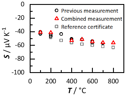
Figure 13 Seebeck coefficient of constantan up to 800 ^∘C. Additionally, all previous measurements and the values of the reference certificate are included.

7 Conclusions

A setup to measure the Seebeck coefficient was successfully integrated into an already existing setup for the measurement of the electrical conductivity and the Hall constant. The ceramic sample holder was optimized using FEM simulations. A primary heating structure was developed to extend the temperature range from 600 up to 800 ^∘C. A secondary heater enables to modulate the temperature distribution within the sample area. The simulations were confirmed by thermography using an IR camera. The contact point temperature was measured by two Au–Pt thermocouples. The design of the thermocouples could be adapted to the new requirements by preliminary tests. Reproducible measurements on constantan and samarium-doped calcium manganate confirmed the successful integration of the setup to measure the Seebeck coefficient. Finally, measurements of the electrical conductivity, the Hall constant, and the Seebeck coefficient of boron-doped silicon and constantan up to 800 ^∘C confirmed the functionality of the entire gauge. In addition, the measurements again demonstrated that even at a sample temperature of 800 ^∘C, the use of permanent magnets is possible with this ceramic sample holder concept.