Integration and evaluation of the high-precision MotionCam-3D into a 3D thermography system

Infrared thermal imaging enables fast, accurate and non-contact measurement of temperature distributions. However, 2D representations of 3D objects often require several images to provide significant information. For such cases, 3D thermograms allow a quick temporal and spatial analysis. In this paper, the integration of an industrial high-precision 3D sensor into a 3D thermography system is presented. The performances of the existing and new systems are assessed and compared by analyzing 3D thermograms of an industry-related test object. The geometry of the obtained point cloud is evaluated by means of a non-referenced point cloud quality assessment approach. It is shown that, in the presence of the spatial resolution and the local curvature, the proposed system performs significantly better than the existing one.

1 Introduction

Infrared thermography is a measurement technique which generates thermal images from the infrared radiation emitted by the object to be measured. These images are called thermograms, and the value of the temperature contained in each pixel is provided by the digital response of the thermal detector elements of the camera. For this purpose, the camera sensor provides radiance-proportional values, which are converted into radiation temperature values using a known emissivity and a calibration function determined by the camera manufacturer. Thermography is an attractive approach to measuring temperature. It is non-invasive, is contactless, and provides a quick response compared with contact thermometers. In addition, thermography cameras provide spatially distributed temperature fields. This technique has been used in various applications, such as in situ detection of defects in chip manufacturing (Bin et al., 2024), the monitoring of additive manufacturing processes (Gardner et al., 2022) or the detection of breast cancer (Greeshma et al., 2023). Nevertheless, 2D thermograms are of limited use in situations where the field of view of the cameras is not able to cover completely the surface of interest or there are hotspots hidden by other objects. Such a planar representation does not allow a detailed analysis and is therefore insufficient for decision-making.

Three-dimensional thermograms are an interesting alternative to overcome this limitation, and a variety of systems have been developed over the past few years. A categorization can be considered with two groups, depending on whether a 3D sensor is used to capture the geometry of the objects or whether an alternative methodology is considered for this. This is the case with Ng and Du (2005), who showed the utility of 3D thermograms for the acquisition of data to validate finite-element-method simulations. The authors presented a method for the projection of the thermograms onto a coordinate system and a reconstruction algorithm based on the octree carving technique. The results allow the surface temperature distribution of a car model to be obtained without the use of a wide set of contact thermometers. Ham and Golparvar-Fard (2013) deployed a commercial hand thermal-imaging camera for generating 3D spatio-thermal models to assess the energy performance of existing buildings. The 3D models were generated with the aid of GPU-based structure-from-motion and multi-view stereo algorithms. Sels et al. (2019) presented a computer-aided design (CAD) matching method for complex objects. The image plane of the thermal image was aligned with the virtual scene of the CAD model to subsequently map pixel-wise the temperature values onto the 3D model. With respect to the 3D sensor group, there is a clear trend towards systems configured with laser scanners and thermographic cameras. Grubišić et al. (2011) presented a system in which the concepts of active and passive thermography were exploited to obtain and inspect 3D models of a human chest for detecting breast cancer.

Lagüela et al. (2011) presented a methodology for texturing the point clouds obtained with a 3D laser scanner. Control points, visible for both the scanner and the thermal-imaging camera, were placed on the scene to obtain the geometrical relationship between the thermogram and the point cloud. Wang et al. (2013) presented a rigidly assembled system. In this case, the temperature values are not represented as RGB values but are assigned directly to the points as non-graphic values. The data from the different sensors are fused by means of a perspective reprojection, which uses the geometrical relationship of the optical components calculated from the assembly. Hellstein and Szwedo (2016) also proposed an assembled system, which was used in the context of active thermography to inspect boat hulls. The system in this case was geometrically calibrated to obtain not only the intrinsic parameters, but also the extrinsic parameters. Costanzo et al. (2014) inspected a historical building with a terrestrial laser scanner and a thermal-imaging camera. A methodology was proposed to align multiple scans of a subcentimeter resolution scanner with a single scan of a submillimeter resolution scanner. The thermal data were assigned to each point in the 3D model by means of a geometrical reprojection. A calibration procedure was carried out to obtain the parameters frame by frame, where at least 11 correspondences were matched to find the relationship between the 3D point cloud and the 2D thermal images. The system obtains the bulk information of the building from the first survey and captures the details with the second survey. The analysis in conjunction with the temperature values allows anomalies and key aspects of the structural integrity of the building to be identified. Campione et al. (2020) also presented a decoupled system in which the depth maps and the thermograms are obtained separately. A set of 3D points is obtained and then filtered by two consecutive exclusion stages to then be texturized with the temperature readings. Afterward, an extrinsic calibration is done frame by frame in order to map the thermograms to the 3D model.

In addition to laser scanners, depth cameras are also an interesting alternative for the construction of portable systems. Vidas and Moghadam (2013) presented a system which employs a ray casting method for the temperature assignment. It takes into account five weighting factors that consider the velocity of the camera, the angle between the ray and the surface normal of the vertex, and the distortions of the optics, among others. This was subsequently upgraded in Vidas et al. (2015) to achieve real-time 3D modeling. Rangel and Soldan (2014) developed a system which fuses the data obtained from a thermal-imaging camera and a low-cost depth sensor. The extrinsic calibration of the cameras was addressed with a calibration target board designed to be visible in the spectral ranges of both sensors. Ordóñez Müller and Kroll (2017) implemented the Kinect Fusion algorithm to extend the creation of 3D models. The model is represented by a volumetric grid composed of unit voxels, which are texturized with the temperature readings of a thermal-imaging camera. Even if the system yields high-3D-fidelity thermograms, objects with sizes larger than $\mathrm{1.28}\text{m}\times \mathrm{1.28}\text{m}\times \mathrm{1.28}\text{m}$ can not be modeled due to the limitation of the memory of the graphics card. Schramm et al. (2020) compared the performance of three point cloud registration algorithms, InfiniTAM (Prisacariu et al., 2017), Kintinuous (Whelan et al., 2015a) and ElasticFusion (Whelan et al., 2015b), to construct 3D thermograms. The best performance was obtained by ElasticFusion in terms of the speed of the calculation and the accuracy of the geometry, and it was therefore the most suitable option for constructing large-scale thermograms in real time. Nevertheless, the models of this system, in contrast to the results that are obtained with the 3D thermography system of Ordóñez Müller and Kroll, do not exhibit the same geometrical fidelity. Although the quality of the 3D point cloud also depends on the registration algorithm, this is mostly influenced by the technology deployed for the measurements. For the system of Schramm et al., the depth sensor can be categorized as a low-cost sensor whose accuracy (<4 cm at 2 m distance) could be inappropriate for some engineering applications.

The implementation of an industrial high-precision 3D sensor (from now on referred to as the “new system”) within the 3D thermography system described in Schramm et al. (2020) (from now on referred to as the “existing system”) is presented in the present paper, which is structured as follows. In Sect. 2, the 3D thermography system is presented. In Sect. 3, the performances of both systems are assessed and compared through an experimental evaluation. In Sect. 4, the conclusions are presented together with an outline of future work.

2 Three-dimensional thermography system

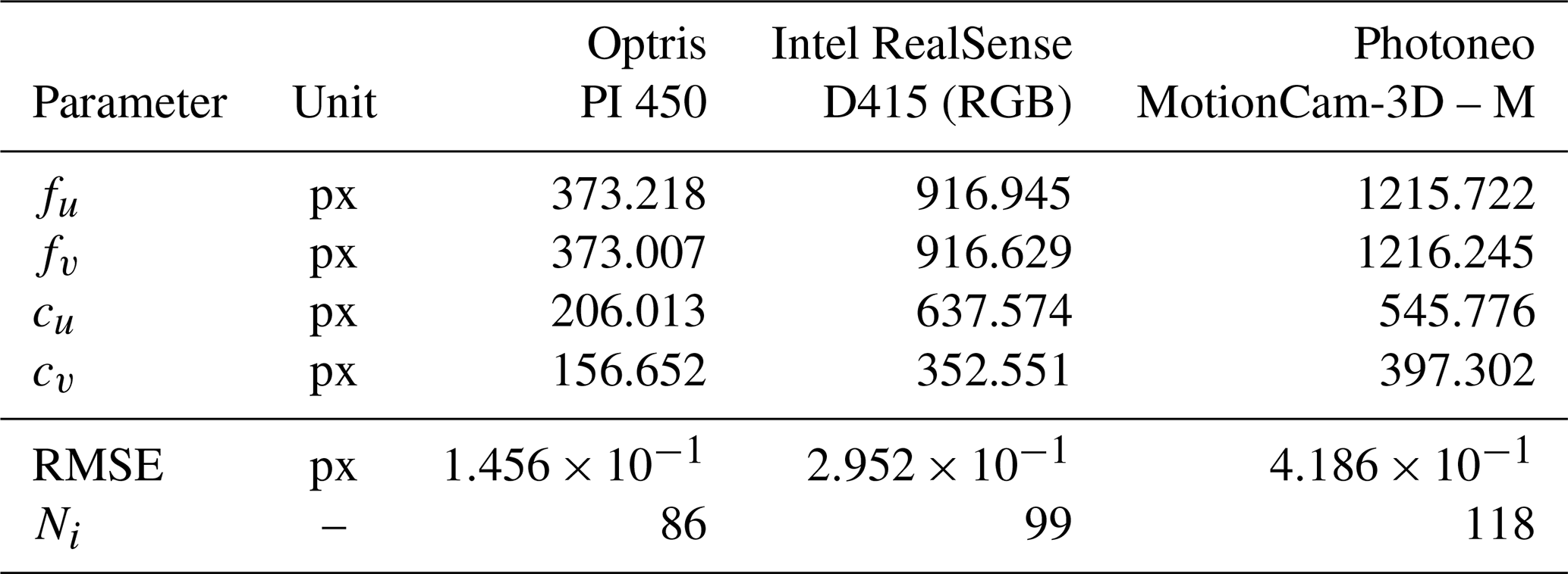
The sensor system consists of a long-wave infrared (LWIR) camera, a depth sensor and an RGB camera, which is assembled in a plexiglass frame to preserve their relative positions. For the existing system (enclosed in the red dotted square in Fig. 1), the depth measurements are carried out by the Intel RealSense D415, which operates with stereo vision technology and a projected near-infrared pattern to enrich features for the stereo matching. The new system operates with the MotionCam-3D from Photoneo, which retrieves the depth measurements from a processed parallel-structured light pattern. The color frames and the thermograms are still obtained by the Intel RealSense D415 and the Optris PI 450 (see Fig. 1). The technical data of the deployed sensors are presented in Table 1.

Figure 1 Three-dimensional thermography system.

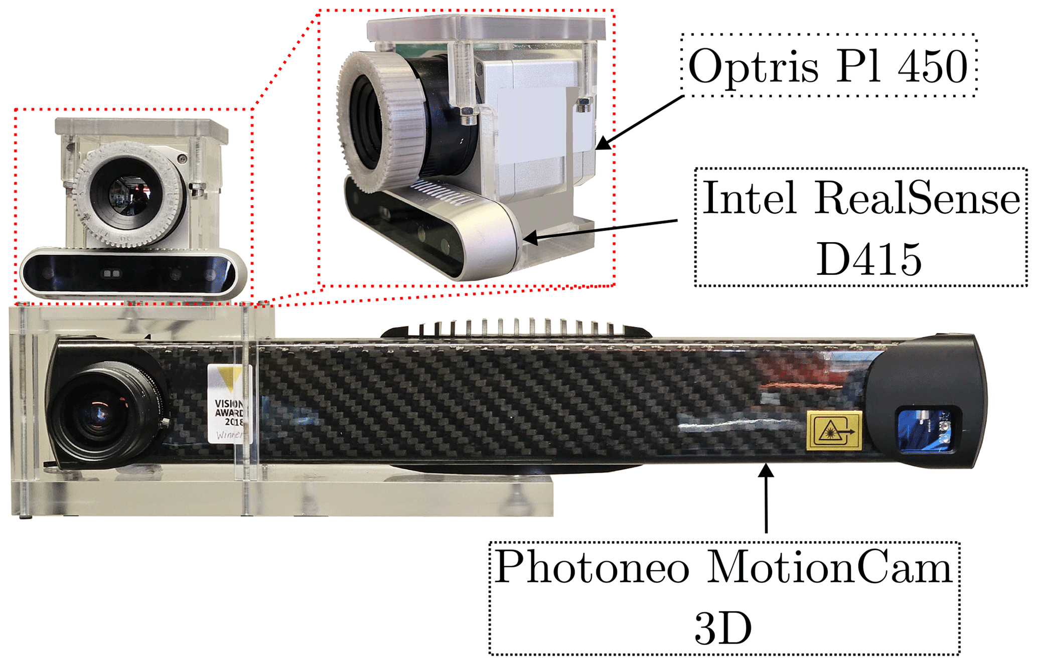
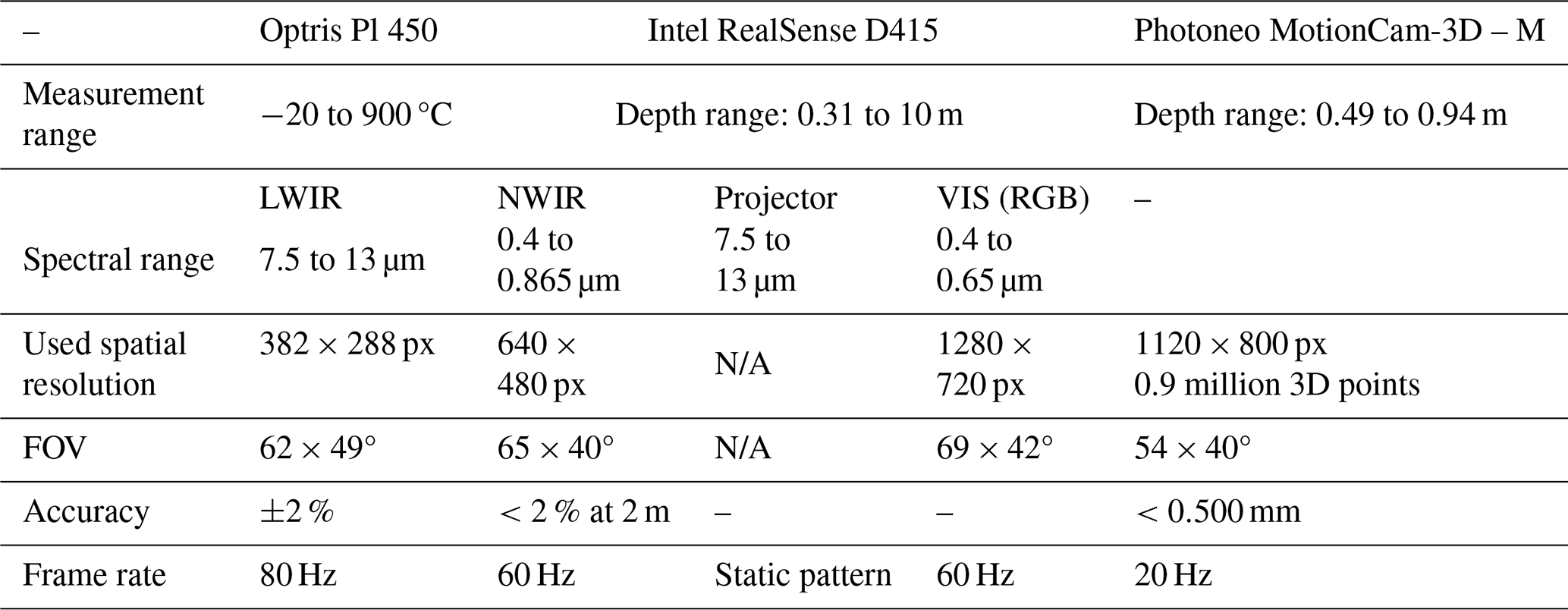
Table 1 Technical data of the sensors deployed for the 3D thermography system (Optris-GmbH, 2024; Intel-RealSense, 2023; Photoneo, 2024). N/A: not applicable.

The 3D thermograms are generated by processing 3D points with the ElasticFusion registration algorithm developed by Whelan et al. (2015b) and extended by Schramm et al. (2020). Basically, ElasticFusion operates by deforming (enlarging) an actual point cloud model with new 3D thermal points. These points are selected from the entire depth map after iteratively searching the point candidates to be merged into the model, based on a convergence criterion of an optimization process. Furthermore, before each depth map is processed, it is texturized with the color and temperature readings, both represented with RGB maps. For that, the program reprojects the thermograms and RGB frames to the plane of the depth image (see Sect. 2.2).

These processing tasks are performed by a developed C++ (CUDA) executable. It exploits the hardware capabilities of a high-end graphics card laptop (GeForce GTX 980M, 4 GB VRAM) by implementing multithreaded computations. This architecture is preferred since it is the most suitable alternative to attain the sufficient computational speed for performing the required calculations. In Fig. 2, an example of the system in operation is presented.

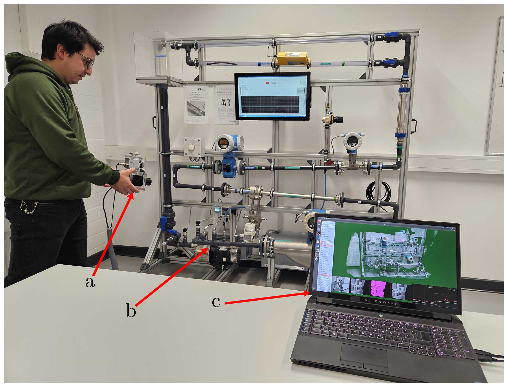
Figure 2 Example of operating the 3D thermography system. In the figure, panel (a) is pointing to the sensor assembly, panel (b) to the test object and panel (c) to a live view of the generated model.

Two main tasks had to be done for the integration of the MotionCam-3D. The first one was the perturbation of the color images caused by the red-light pattern of the MotionCam-3D, which was done by setting the red component of the color vector to 0. The second one was the temporal synchronization of the three cameras. As the postprocessing features of the MotionCam-3D introduce a time delay into the depth frames, the system must search backwards in the temperature and color buffers for the frames which match the last depth measurement in time. When the three images are temporally quasi-aligned, they are processed by the extended ElasticFusion algorithm.

2.1 Geometric model

The pinhole model was employed to represent the relation between an object point Q[X_c Y_c Z_c] in the 3D world and the point q[u v] in the 2D image:

$$\begin{array}{}\text{(1)}& {\displaystyle }\left[\begin{array}{c}u\\ v\\ \mathrm{1}\end{array}\right]{\displaystyle }={\displaystyle \frac{\mathrm{1}}{Z_{\mathrm{c}}}}\underset{\mathbf{M}}{\underbrace{\left[\begin{array}{ccc}{f}_u& \mathrm{0}& c_u\\ \mathrm{0}& f_v& c_v\\ \mathrm{0}& \mathrm{0}& \mathrm{1}\end{array}\right]}}\left[\begin{array}{c}{X}_{\mathrm{c}}\\ Y_{\mathrm{c}}\\ Z_{\mathrm{c}}\end{array}\right],\end{array}$$

where the camera matrix is denoted by M, the focal length scaling factors are f_u and f_v (px), and the image centers are c_u and c_v (px), which are obtained from the intrinsic calibration of each camera: see Sect. 2.2.

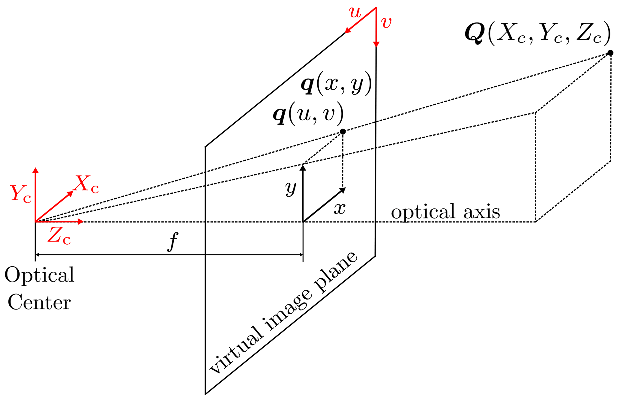
Figure 3 Schematic representation of the pinhole model, based on Schramm et al. (2021a).

In order to formulate the camera model with reference to an overall origin, the data collected from the color camera and the thermal-imaging camera are reprojected from the Cartesian coordinate system “csi” of each camera to a reference point “csu”, which in this case is placed at the optical center of the MotionCam-3D. The coordinates of the reference point are given by

$$\begin{array}{}\text{(2)}& {\displaystyle }\left[\begin{array}{c}{X}_{\mathrm{csi}}\\ Y_{\mathrm{csi}}\\ Z_{\mathrm{csi}}\end{array}\right]{\displaystyle }=\underset{\mathbf{W}=\left[\mathbf{R}\right|\mathit{t}]}{\underbrace{\left[\begin{array}{cccc}{r}_{\mathrm{11}}& r_{\mathrm{12}}& r_{\mathrm{13}}& |{\mathit{t}}_{\mathrm{1}}\\ r_{\mathrm{21}}& r_{\mathrm{22}}& r_{\mathrm{23}}& |{\mathit{t}}_{\mathrm{2}}\\ r_{\mathrm{31}}& r_{\mathrm{32}}& r_{\mathrm{33}}& |{\mathit{t}}_{\mathrm{3}}\end{array}\right]}}\left[\begin{array}{c}{X}_{\mathrm{csu}}\\ Y_{\mathrm{csu}}\\ Z_{\mathrm{csu}}\\ \mathrm{1}\end{array}\right],\end{array}$$

where R is the rotation matrix and t is the translation vector, which were obtained by means of a geometrical extrinsic calibration, since it is not feasible to locate the coordinate origin of each camera by direct length measurements.

2.1.1 Point cloud texturization

As was previously mentioned, the frames of the color camera and the thermal-imaging camera are represented in the model with RGB values. In the case of the thermograms, the temperature scalar values are transformed to the RGB vectors by means of a look-up table. For the texturization of the point cloud, the frames of both cameras are first resized to the dimensions of the ones delivered by the depth camera. Afterward, these RGB-represented frames are reprojected to the overall coordinate system csu by the combination of Eq. (1) with Eq. (2):

$$\begin{array}{}\text{(3)}& {\displaystyle }{\mathbf{q}}_r^{\prime }={\mathbf{M}}_r\cdot {\mathbf{W}}_r\cdot \left({\mathbf{M}}_d^{-\mathrm{1}}\cdot Z_{\text{c}}\cdot {\mathbf{q}}_d\right),\end{array}$$

where r corresponds to the color or thermal-imaging camera and d is the depth camera.

2.2 Geometric camera calibration

The intrinsic and extrinsic calibrations were performed using the coded target presented and discussed in Schramm et al. (2021a). This target improves the boundary detection, reduces the uncertainty of the geometric calibration, and still meets the requirement of being observable in the considered spectral range (LWIR, NWIR and VIS) with a sufficient contrast-to-noise ratio, as is explained in Schramm et al. (2021b).

The results for the intrinsic calibration are presented in Table 2; they were obtained by considering a different number of images N_i for each camera. The root-mean-squared error (RMSE) of the Euclidean distance between the detected point position q and the reprojected point q^′ was calculated to evaluate the quality of the calibration:

$$\begin{array}{}\text{(4)}& {\displaystyle }\text{RMSE}=\sqrt{{\displaystyle \frac{\mathrm{1}}{N_{\mathrm{f}}}}\sum _{n=\mathrm{1}}^{N_{\mathrm{f}}}\left|\right|{\mathit{q}}_n-{\mathit{q}}_n^{\prime }|{|}^{\mathrm{2}}},\end{array}$$

where N_f is the number of features to be identified. For the three cameras, values of the RMSE on the order of less than 1 pixel were obtained. Compared with the values reported in Schramm et al. (2021b) for the uncoded chessboard target, reductions of about 45 % and 33 % were achieved for the color camera and the infrared thermal-imaging camera, respectively.

Table 2 Results of the intrinsic calibration.

The results for the extrinsic calibration are presented in Table 3. The coordinate system of the MotionCam-3D was chosen to hold the global coordinate system of the 3D thermography system. This implies that the frames recorded by the color camera and the thermal-imaging camera are reprojected to this point by Eq. (2). As with the intrinsic calibration, a reduction of the RMSE was achieved by about 10 % for the thermal-imaging camera with respect to the reported RMSE in Schramm et al. (2020). No comparisons are presented for the RGB camera since it was not extrinsically calibrated in Schramm et al. (2020).

Table 3 Results of the extrinsic calibration. The values are taken from each individual camera coordinate system to the coordinate system of the MotionCam-3D.

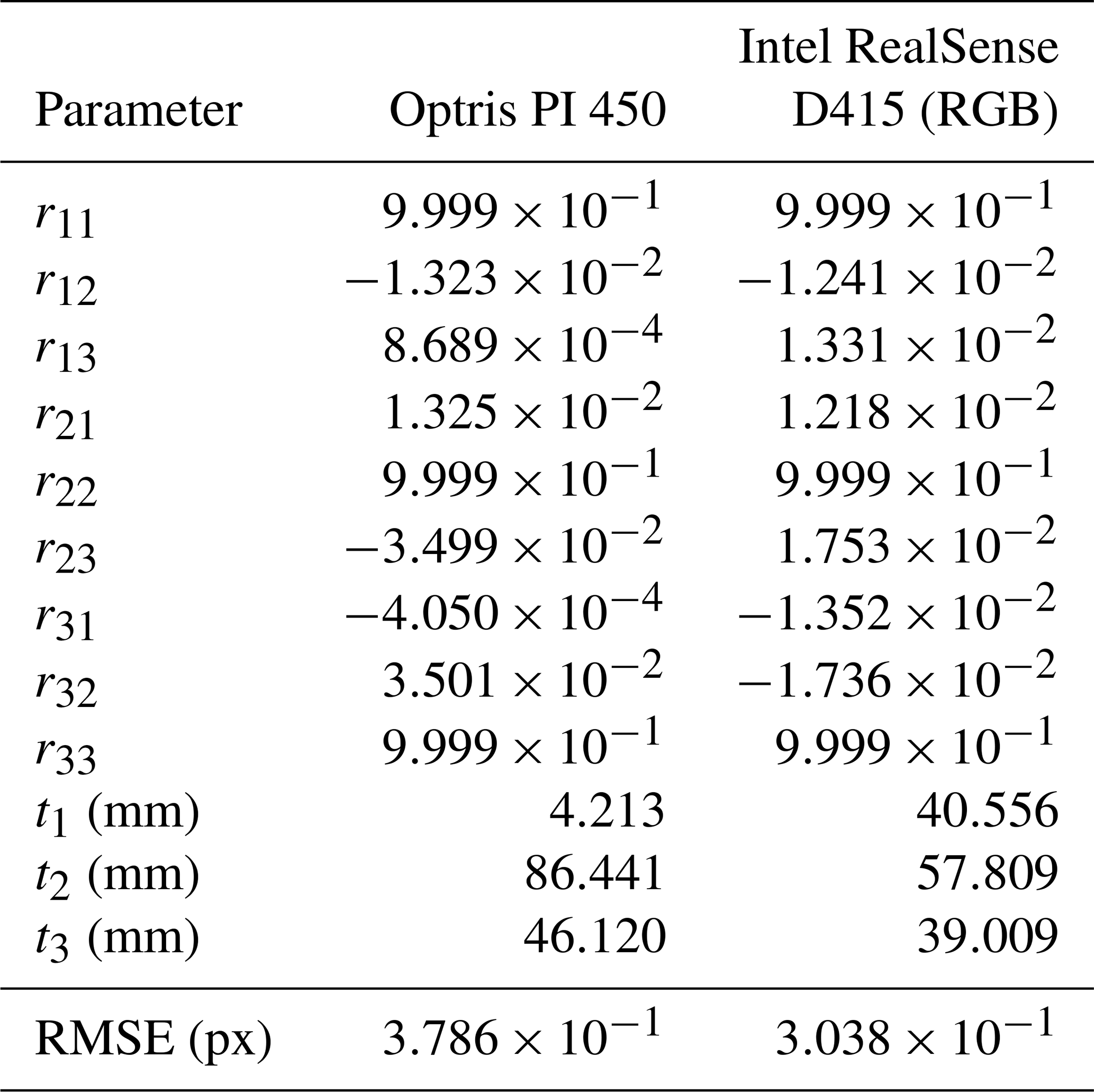
By visual inspection, it was possible to confirm that the values found for the rotation and translation matrices describe the relative locations between the coordinate systems csu and csi.

3 Experimental evaluation of the 3D thermography systems

An experimental study was carried out in order to evaluate and compare the models obtained with each system. For this purpose, a geometrical test object was inspected six times and eight times with the existing and new systems, respectively. The obtained models were analyzed qualitatively and quantitatively in order to evaluate the geometrical fidelity and the quality of the point clouds. The results presented below only correspond to one model obtained with each system, since a similar behavior is obtained from the other models.

3.1 Test object

The flow measurement test bench presented in Fig. 4 was selected to be the object under study. It was chosen because, on the one hand, its design enables the study of the reproduction of both flat and curved regions of varying sizes, arranged at different distances in a non-predefined manner. On the other hand, the components of this test bench, such as pumps and instruments, which are heated by their operation, are elements found in typical industrial assemblies. Likewise, these elements and their joints, such as PVC pipes and metal flanges, are made of different materials (some of them with paint coating) whose emissivities ϵ differ notably, which causes a visual contrast in the thermograms delivered by the infrared camera. Additionally, the thermal contrast was increased for the experimental study by pumping hot water through the test bench.

Figure 4b presents a typical 3D thermogram obtained for the test object with the new system. In the 3D thermogram, one of the hottest sections of the pipeline is observed in the upper-left region (label 1 in Fig. 4a), which corresponds to the water intake point of the system. The temperature decreases slightly downstream (label 2) in the pipe leading to the pump and increases again after passing through this device (label 4). Correct temperature readings were not expected from the measurements on the metal parts, such as the body of the mass meter (label 5) or the shiny metal pipe above it (label 7), since the emissivities of these surfaces (ϵ<0.3) differ from the one set for the experimental study (ϵ=1). However, the green sticker on the metal pipe (where the arrow of label 7 points) has a similar emissivity value (ϵ>0.85). It can therefore be concluded that these readings do correspond to the surface temperature of the pipe at this point. It is also important to note that the heating of the pump motor (label 3) can also be observed in the 3D thermogram.

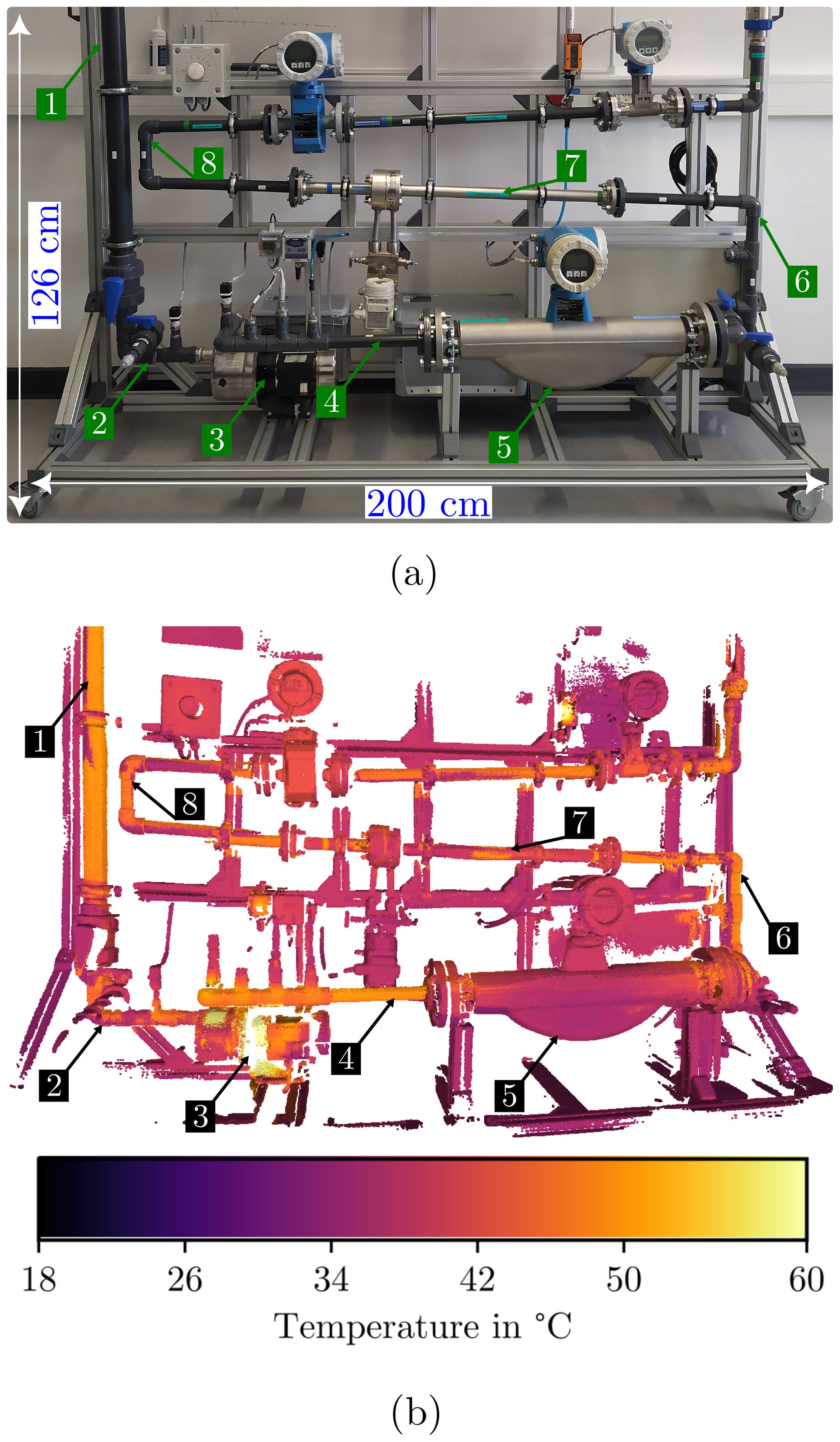
Figure 4 Test object for the evaluation (a) and its respective 3D thermogram obtained with the new system (b).

3.2 Qualitative assessment

Figure 5 presents a comparison of the obtained point clouds for some regions of the test object. A visual improvement of the quality of the geometry is observed with the MotionCam-3D. In the upper row it can be noted that the new system provides straighter lines and flatter surfaces, as can be seen in the regions corresponding to the frame of the test object. Moreover, since the MotionCam-3D retrieves more points, the resolution of the model is consequently increased, enabling a better identification of the details of the object.

Exemplary details of typical scenarios of differences observed in the point clouds obtained with both systems are presented in the bottom row of Fig. 5. For the existing system, the edges of some objects are not clearly distinguishable, and the associated components can be misinterpreted. This has two main repercussions. On the one hand, a situation arises in which free regions between nearby bodies are filled with scattered points that create artificial surfaces. This can be observed when two components are merged, as in rectangle 1 with the two contiguous sensors, rectangle 2 with the parallel vertical tubes and rectangle 4 with the cables coming out of the regulator. On the other hand, the section changes are not perceived, making the contours of the objects look continuous. This is the case for rectangles 2 and 3 with the end sections of the fittings, the clamp in rectangle 5 and the knob on the regulator in rectangle 6. The fidelity of the surface alignment is addressed with the blue rectangles. The model produced by the existing system (column b) fails to retrieve a correct face orientation between the front of the regulator (where the knob is placed) and the side face. As can be observed in column c, these artifacts are no longer observed for the new system, and the representation of the measurement object is more consistent with their actual geometry (column a).

Nevertheless, it is common to observe bodies with incomplete regions in the models produced by the new system (see rectangle 7). This is due to the fact that the measurement volume of the MotionCam-3D is limited by a narrower distance compared with the one of the Intel RealSense camera. Even if with the existing system fewer points are integrated into the model, more regions can be covered with this sensor.

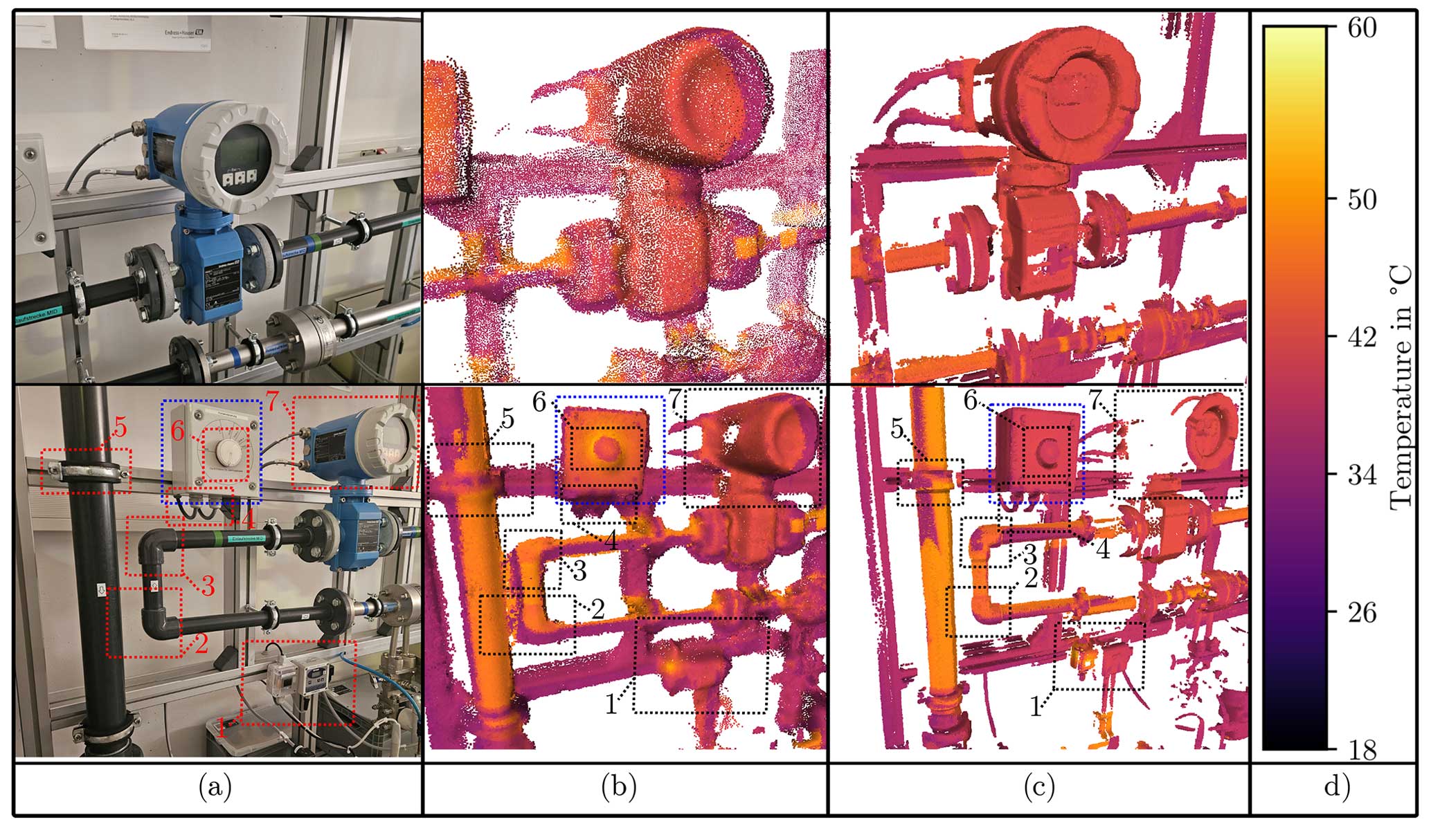
Figure 5 Visual comparison of the models obtained for the test object with the existing system (b) and the new system (c). Corresponding photographs of the analyzed sections of the test bench are presented in panel (a).

3.3 Quantitative assessment

The quality of point clouds can be measured through subjective and objective methods according to Dumic et al. (2018). Regarding the subjective methods, these are the well-known international standard ITU-R BT.500-13 (International Telecommunication Union/ITU-R Radiocommunication Sector of ITU, 2012), which defines a set of protocols to collect a mean opinion score, or the methods based on user interaction with the raw point clouds (Zhang et al., 2014; Alexiou and Ebrahimi, 2017).

The objective methods can be assigned to two groups. The first are recognized as full-reference methods which measure the point cloud quality using a reference model (e.g., Mekuria and Cesar, 2016; Tian et al., 2017). These are mostly used for assessing downsampled or compressed point clouds. The second are known as non-reference methods and establish quality metrics based on local geometry information (Mallet et al., 2011; Zhang et al., 2022).

In this case study, the subjective methods are not of interest, since they do not aim to measure the usability of the texturized information in the 3D thermograms, which in this case are the temperature values represented by RGB values. The full-reference methods were also not an option because it is not possible to define a ground truth that permits a fair comparison for both systems. The non-reference methods still address these two limitations and fit the study requirements, which are the establishment of indicators to evaluate the equivalence of the point clouds with the geometry of the recorded objects and the use of the 3D thermograms for further applications.

Most of the non-reference approaches are based on the analysis of the local surface variation. From a point cloud $P=\mathit{\{}{\mathit{p}}_i{\mathit{\}}}_{i=\mathrm{1}}^N$, a neighborhood P_Nbi of each point p_i is obtained by employing the k-nearest-neighbor (k-NN) algorithm, using the Euclidean distance metric. For the following analysis, the size of P consists of $N=\mathrm{3.76}\times {\mathrm{10}}^{\mathrm{5}}$ and $N=\mathrm{1.82}\times {\mathrm{10}}^{\mathrm{6}}$ points for the existing and new systems. The key goal is to measure how close the member points are to the centroid ${\widehat{\mathit{p}}}_i$ of P_Nbi and to establish whether the shape of the local neighborhood conforms to the actual shape of the real object in the respective zone.

3.3.1 Dispersion of the points in the neighborhoods

One-hundred points were randomly selected to measure the spatial distribution in their respective neighborhoods. The standard deviation along each coordinate axis $\mathit{\{}x,y,z\mathit{\}}$ was computed. This was not performed on the entire point cloud because it is computationally intensive. Figures 6 to 8 present the histograms for the standard deviations σ_x, σ_y, and σ_z using k=10 members for each neighborhood. In all three cases, the results for the new system show a narrower distribution, with an approximate range of 1 mm, whose expected value is below 1 mm. In the case of the existing system, the range of the distribution was from 4 to 6 mm, and the most probable value tends towards 2 mm. This suggests that the new system provides improved geometric accuracy due to the local agglomeration of points in narrower neighborhoods, which is consistent throughout the model.

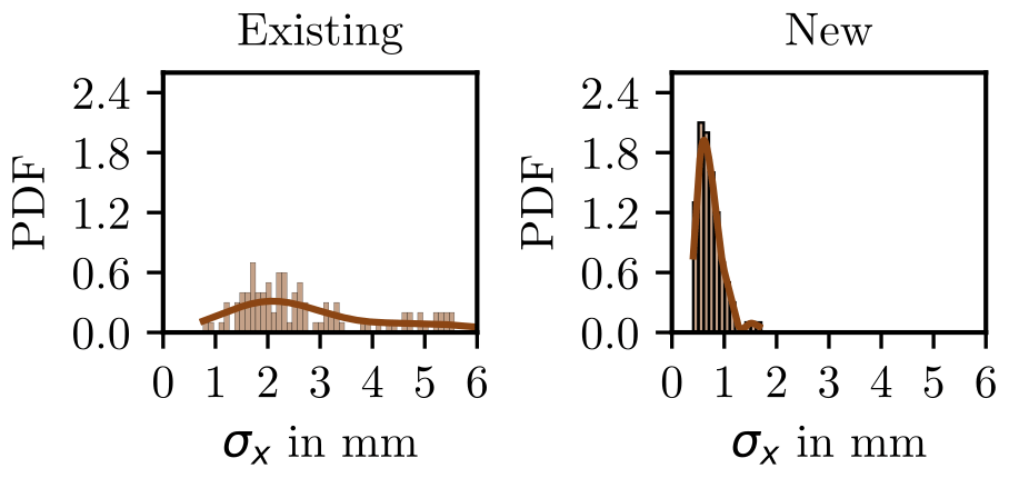
Figure 6 Probability density function of σ_x for each neighborhood of 100 randomly selected points. A bin width of 0.1 mm was selected for generating the histogram. The neighborhoods consist of k=10 members.

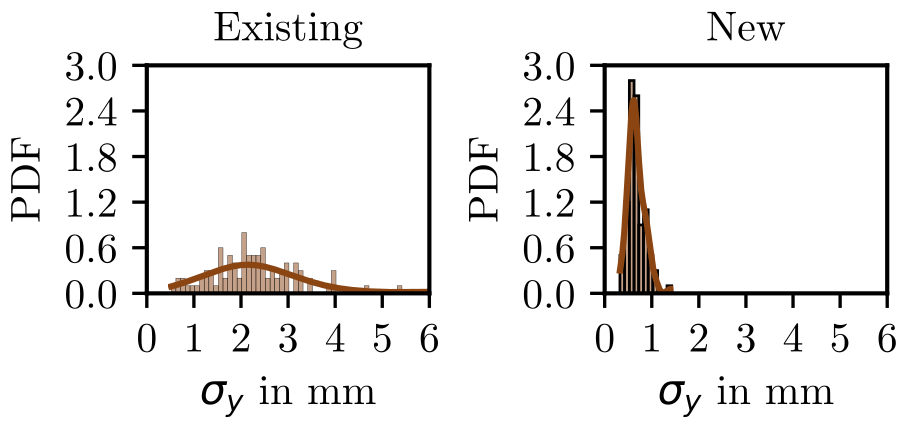
Figure 7 Probability density function of σ_y for each neighborhood of 100 randomly selected points. A bin width of 0.1 mm was selected for generating the histogram. The neighborhoods consist of k=10 members.

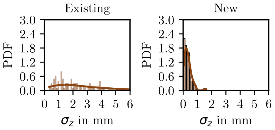
Figure 8 Probability density function of σ_z for each neighborhood of 100 randomly selected points. A bin width of 0.1 mm was selected for generating the histogram. The neighborhoods consist of k=10 members.

3.3.2 Local roughness

Hoppe et al. (1992) proposed a method to assess the shape of the point neighborhoods. It consists of the computation of the empirical covariance matrix C_i:

$$\begin{array}{ll}\text{(5)}& {\displaystyle }{\mathbf{C}}_i& {\displaystyle }={\displaystyle \frac{\mathrm{1}}{k}}\sum _{j=\mathrm{1}}^k\left({{\mathit{p}}_n}_j-{\widehat{\mathit{p}}}_i\right){\left({{\mathit{p}}_n}_j-{\widehat{\mathit{p}}}_i\right)}^T,{\displaystyle }& {\displaystyle }\mathit{\{}{{\mathit{p}}_n}_{\mathrm{1}},\mathrm{\dots },{{\mathit{p}}_n}_k\mathit{\}}\in P_{\mathrm{Nbi}},\end{array}$$

where ${{\mathit{p}}_n}_j$ and ${\widehat{\mathit{p}}}_i$ are Cartesian coordinate vectors and represent the jth member and the mean of the neighborhood P_Nbi, respectively. The eigenvector problem is solved for all points p_i in P:

$$\begin{array}{}\text{(6)}& {\displaystyle }{\mathit{C}}_i\cdot {\mathit{v}}_l={\mathit{\lambda }}_l\cdot {\mathit{v}}_l,l\in \mathit{\{}\mathrm{1},\mathrm{2},\mathrm{3}\mathit{\}},\end{array}$$

with the eigenvectors $({\mathit{v}}_{\mathrm{1}},{\mathit{v}}_{\mathrm{2}},{\mathit{v}}_{\mathrm{3}})$ and the corresponding eigenvalues $({\mathit{\lambda }}_{\mathrm{1}}>{\mathit{\lambda }}_{\mathrm{2}}>{\mathit{\lambda }}_{\mathrm{3}})$. The variation of p_i along the direction of v_l is represented by λ_l (Pauly et al., 2002), and thus the shape of the neighborhood can be evaluated. The curvature

$$\begin{array}{}\text{(7)}& {\displaystyle }\mathrm{Cur}\left({\mathit{p}}_i\right)={\displaystyle \frac{{\mathit{\lambda }}_{\mathrm{3}}}{{\mathit{\lambda }}_{\mathrm{1}}+{\mathit{\lambda }}_{\mathrm{2}}+{\mathit{\lambda }}_{\mathrm{3}}}}\end{array}$$

proposed by Pauly et al. (2002), Rusu (2009) and Weinmann et al. (2013) provides information about the local roughness (Zhang et al., 2022) and was calculated for this study. The size of the neighborhoods was also set fixed at 10 members (k=10), as was done by Zhang et al. (2022) and Hackel et al. (2016). This is fair for assessing both systems since the eigenvalues do not depend on the scale, rotation or translation (Jutzi and Gross, 2009).

Figure 9 presents an example of a typical neighborhood obtained with both systems. The components of the coordinate vectors were redefined according to the following normalization:

$$\begin{array}{}\text{(8)}& {\displaystyle }{F}^{\prime }={\displaystyle \frac{F-\mathrm{mean}\left(F\right)}{\max \left(F\right)-\min \left(F\right)}},\end{array}$$

where F corresponds to $\mathit{\{}x,y,z\mathit{\}}$. The example of the new system shows that the points p_i are more concentrated around the centroid and are closer to the regression plane. If a surface were reconstructed from these, it would be observed that its roughness is lower in this case. The calculation of the curvature Cur confirms this. The computation of the eigenvalues λ_l with Eq. (7) indicates a reduction of 3 orders of magnitude for the new system.

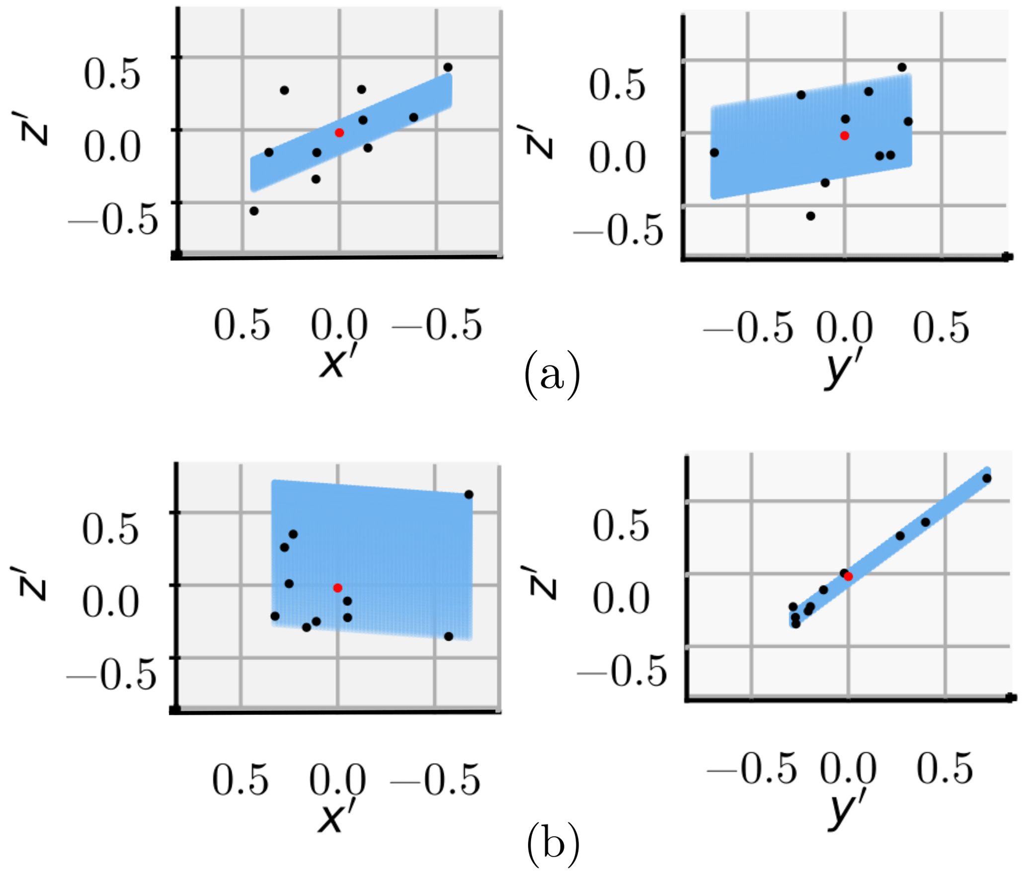
Figure 9 Example of a typical neighborhood from the point clouds obtained with the existing (a) and new (b) systems. The units of the axes were modified according to Eq. (8). The values of $\mathit{\{}{\mathit{\lambda }}_{\mathrm{1}},{\mathit{\lambda }}_{\mathrm{2}},{\mathit{\lambda }}_{\mathrm{3}},\mathrm{Cur}\mathit{\}}$ for P_Nbi in panels (a) and (b) are $\mathit{\{}\mathrm{7.1}\times {\mathrm{10}}^{-\mathrm{6}},\mathrm{4.6}\times {\mathrm{10}}^{-\mathrm{6}},\mathrm{3.6}\times {\mathrm{10}}^{-\mathrm{7}},\mathrm{3.1}\times {\mathrm{10}}^{-\mathrm{2}}\mathit{\}}$ and $\mathit{\{}\mathrm{5.8}\times {\mathrm{10}}^{-\mathrm{5}},\mathrm{3.7}\times {\mathrm{10}}^{-\mathrm{6}},\mathrm{1.3}\times {\mathrm{10}}^{-\mathrm{9}},\mathrm{2.2}\times {\mathrm{10}}^{-\mathrm{5}}\mathit{\}}$, respectively. The blue plane was obtained from a linear regression fitting, and the red point corresponds to the centroid of the neighborhood.

This is consistent with all the point clouds delivered by both systems, whose results are presented in Fig. 10. The local curvature around the registered points was notably reduced with the implementation of the MotionCam-3D. The statistical distribution of this indicator shows a trend towards the ideal value (Cur=0) of this feature for the entire data set. Correspondingly, smoother surfaces could be obtained from these point clouds, which means that a better approximation to the real object was achieved.

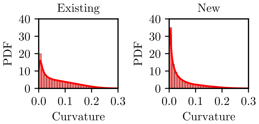
Figure 10 Probability density functions of the local curvature. A bin width of 0.01 was used for plotting the histograms.

3.3.3 Sizes of the surface elements

In a strict sense, the models obtained by Elastic Fusion are conceptualized with a surface discretization entity known as Surfel (Pfister et al., 2000). These are unordered point primitives without explicit connectivity, and for the extended system, Schramm et al. (2020) combine the following attributes: position, normal vector, weight, color and temperature values textured with RGB vectors, time stamps, and radius r_s. Surfel is associated with circular surface elements whose radius r_s is calculated as follows:

$$\begin{array}{}\text{(9)}& {\displaystyle }{r}_{\mathrm{s}}={\displaystyle \frac{d\cdot \sqrt{\mathrm{2}}}{\frac{f_u+f_v}{\mathrm{2}}\cdot \left|n_z\right|}},\end{array}$$

with d the depth measurement, f_u and f_v the focal length scale factors (see Sect. 2.1) and $\left|n_z\right|$ the z component of the estimated normalized normal vector. During the model creation, ElasticFusion determines the value of r_s to minimize the holes between neighboring surface elements (Weise et al., 2009; Keller et al., 2013; Salas-Moreno et al., 2014). The statistical distributions are presented in Fig. 11. As for the other metrics, the surface element size of the model obtained with the new system also exhibits a narrower range and an expected value towards a smaller radius. This indicates that the resolution of the models has increased with the new system by more than 2 times, as was expressed before. It would be expected that using the 3D thermograms of the new system for calculating the surface heat dissipation of inspected bodies (see Schmoll et al., 2022) should deliver more accurate results due to the possibility of obtaining a mesh with smaller elements.

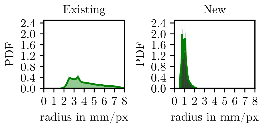
Figure 11 Probability density functions of the local surface radius. A bin width of 0.01 mm was used for plotting the histograms.

4 Conclusions

This paper has presented the integration of a MotionCam-3D into a 3D thermography system. The new system was geometrically calibrated with a coded target, obtaining an overall improvement of the root-mean-squared reprojection error of the intrinsic and extrinsic calibrations, compared with the results obtained in Schramm et al. (2021b, 2020).

The performances of the existing and new systems were evaluated through a qualitative and quantitative assessment of the resulting point clouds. A flow measurement test bench was selected as a test object and therefore modeled with both systems. On the one hand, curved and flat surfaces at different sizes can be modeled from this object. On the other hand, it includes equipment and instruments distinguishable in industrial installations. To enhance the thermal contrast, hot water was made to flow through the test bench. The presented 3D thermogram showed heating of operating components and sections of the test object with relevant temperature differences.

The qualitative inspection suggests a reduction of the number of scattered points around the surfaces and better identification of the details of the body, such as the section change in the tube fittings (see Fig. 5), fewer artifact surfaces and an increase in the spatial resolution, all as a consequence of the deployment of the MotionCam-3D. This has a significant impact on the interpretability of 3D thermograms. The ability to accurately locate atypical regions in the thermal distribution of objects, such as unexpected heat or sink sources (e.g., hotspots), depends directly on the quality of the geometrical representation of the models.

The quantitative assessment was carried out with a non-reference method, calculating local statistics of point neighborhoods. A sample of 100 points was selected to estimate the spatial distribution of the point neighbors around its centroid in every neighborhood. The results showed that using the new system results in models with lower standard deviations in the three directions. This means that the greater spatial resolution of the MotionCam-3D has the expected effect of increasing the geometric accuracy of the created model. The local surface roughness was also studied for all the point clouds, considering a principal component approach. The results also showed a decrease in the local surface variation, resulting in less dispersion throughout the entire geometry.

The Surfel radius of the 3D thermograms was also considered in the evaluation. The results showed that the size of these surface units has decreased by a factor of 2 to 3. This suggests that the point clouds obtained with the new system are more useful for post-applications, such as creating meshes for calculating the surface heat dissipation and computing the measured temperature values, as presented in Schmoll et al. (2022). This will be assessed in a future work.

For future work, the following improvement of the 3D thermography system will be addressed.

• Spatiotemporal calibration of the system: Vidas et al. (2013) presented a methodology to determine the timing offset between the clocks of the sensors. This will improve the assignment of the temperature values in the point cloud.

• Data fusion of depth sensors: similar to Costanzo et al. (2014), the dual deployment of the Intel RealSense camera and the MotionCam-3D can be considered for obtaining point clouds. The first sensor is expected to exploit its field of view and the second its geometric accuracy.

Finally, the system will be tested in industrial scenarios in order to evaluate its performance and the usability of its results.