the Creative Commons Attribution 4.0 License.
the Creative Commons Attribution 4.0 License.
 | 09 Jul 2024
Extraction of nanometer-scale displacements from noisy signals at frequencies down to 1 mHz obtained by differential laser Doppler vibrometry
Dhyan Kohlmann
Marvin Schewe
Hendrik Wulfmeier
Christian Rembe
Holger Fritze
A method is presented by which very small, slow, anharmonic signals can be extracted from measurement data overlaid with noise that is orders of magnitude larger than the signal of interest. To this end, a multi-step filtering process is applied to a time signal containing the time-dependent displacement of the surface of a sample, which is determined with a contactless measurement method, differential laser Doppler vibrometry (D-LDV), at elevated temperatures. The time signal contains the phase difference of the measurement and reference laser beams of the D-LDV, already greatly reducing noise from, e.g., length fluctuations, heat haze, and mechanical vibrations. In postprocessing of the data, anharmonic signal contributions are identified and extracted to show the accurate displacement originating from thickness changes of thin films and related sample bending. The approach is demonstrated on a Pr0.1Ce0.9O2−δ (PCO) thin film deposited on a single-crystalline ZrO2-based substrate. The displacement extracted from the data is ca. 38 % larger and the uncertainty ca. 35 % lower than those calculated directly from the D-LDV spectrum.
- Article
(1401 KB) - Full-text XML
- BibTeX
- EndNote


The evaluation of anharmonic signals overlaid with noise that is greater than the signal of interest is of great interest because in fields as diverse as mechanical vibrations, acoustics (Klippel, 2005), and optics, observable phenomena are often not purely harmonic but only approximated or assumed as such. Especially in astronomy, signals from, e.g., exoplanet detection (Hara and Ford, 2023), are often periodic but not harmonic and overlaid with background noise, which constitutes a poor detection limit. One of the goals of this paper is to point out how this detection limit can be further reduced with respect to other methods or previous applications of the same measurement principle as used here. Another goal is to demonstrate how non-harmonic displacements, which are not expressed in a single peak in the Fourier spectrum, can be accurately extracted from the data.
The application of the evaluation method developed here is demonstrated on interferometric measurements of the displacement of a sample surface, which is driven by chemical expansion of a Pr0.1Ce0.9O2−δ thin film at high temperatures.
1.1 Non-stoichiometry and chemical expansion
This sample system and this phenomenon are well suited for demonstrating the new approach because the displacement is small, slow, anharmonic, and overlaid with much noise. In addition, there is an interest to better understand the chemical expansion of thin films because in industrial high-temperature applications (chemical reactors, combustion engines, fuel cells, catalyzers, etc.), the active material in many components, e.g., sensors, or protective coatings are often implemented as thin oxide films (Preux et al., 2012). During deployment, these thin films are exposed to varying chemical environments, which cause, e.g., in reducing atmospheres an oxygen deficit in oxides. This change in composition is often accompanied by a proportional, relative change in lattice parameter, called chemical expansion, εC (Bishop et al., 2014; Bishop, 2013; Schmitt et al., 2020; Marrocchelli et al., 2012). If the thin film expands but not its bonded substrate, or if they expand differently, a mechanical stress arises. The stress leads to bending of the sample, which might lead to delamination and cracking of the thin films, equalling device failure and thus contributing to limited lifetimes of said devices (Atkinson, 2017). Better understanding of the chemical expansion in thin films and the deformation of the entire macroscopic structure is therefore of industrial interest. The chemical expansion can be determined by measuring the displacement of the surface of a sample, which is the sum of the film thickness change and the bending of the substrate the film adheres to.
The detection of this displacement is challenging for several reasons. Firstly, the chemical expansion is coupled to the migration of oxygen vacancies, the equilibration time of which can be up to several hours (Kogut et al., 2021, 2022), making the displacement due to chemical expansion smaller and slower than that resulting from temperature instabilities (Kohlmann et al., 2023a). Second, since the transport of oxygen vacancies is thermally activated with activation energies of about 0.7 eV (Bishop et al., 2011b), the experiment must be conducted at elevated temperatures, which is inherently challenging because of, e.g., thermal strain and, in the case of optical measurement, heat haze and length fluctuations. Another reason why the displacement is difficult to measure is its size: the relative change in lattice parameter upon partial removal of oxygen is at most a few percent (Bishop et al., 2014), meaning the thickness change of a thin film is at most a few tens of nanometers. Finally, it is commonly non-linear because the oxygen deficit δ approaches chemical equilibrium. Consequently, the chemical expansion and accompanying surface displacement of a sample in response to a harmonic (sinusoidal) excitation are non-harmonic, meaning that it possesses the same periodicity as the excitation but is not sinusoidal.
Each of these four reasons constitutes a demand for a technique which allows for the detection of slow, small, anharmonic displacements in noisy environments. A way of detecting them is laser Doppler vibrometry (LDV), as demonstrated in Schmidtchen et al. (2018), Wulfmeier et al. (2022), and Kohlmann et al. (2023a), which is especially well suited for high-temperature applications. It provides a contactless, interferometric measurement of displacements, which does not influence the sample or its excitation in any way. A new LDV approach which has been developed by the authors is high-temperature differential laser Doppler vibrometry (D-LDV) (Schewe et al., 2023; Kohlmann et al., 2023a, b). The differential approach already suppresses parasitic displacements in the raw, untreated data by exposing both the measurement arm and the reference arm of the interferometer to the same disturbances, largely canceling themselves out in the interference signal. In Schewe et al. (2023), the hardware is presented, focusing on the ability to suppress noise at low frequencies. In Kohlmann et al. (2023b), the applicability of D-LDV is demonstrated at high temperatures and low frequencies down to the megahertz (mHz) range, detecting the displacement of a thin-film praseodymia-ceria (PCO) sample. Here, the data post-processing procedure already applied in Kohlmann et al. (2023b) shall be presented in detail, resulting in the ability to observe the displacements in the time domain, i.e., in a time signal, as opposed to in the frequency domain, i.e., the Fourier transform of the time signal.
As a model material, PCO is chosen because it is well understood and exhibits a plateau of the oxygen partial pressure dependent non-stoichiometry (see Fig. 1) and therefore a plateau of the chemical expansion. This non-linear answer function of the chemical expansion to makes detectable displacements inherently anharmonic as a function of time if the electrochemical excitation is itself harmonic and covers the plateau region as well as the non-plateau region, as in Wulfmeier et al. (2022), Kohlmann et al. (2023a, b), and Swallow et al. (2017).
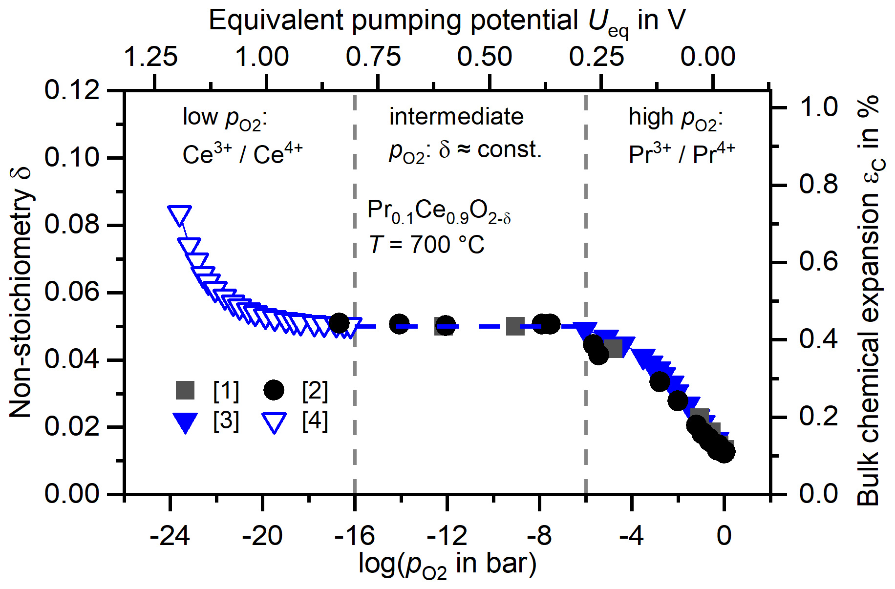
Figure 1The non-stoichiometry δ in Pr0.1Ce0.9O2−δ at T = 700 °C as a function of oxygen partial pressure (bottom abscissa), as stated in the literature. Top abscissa: Nernst potential U corresponding to at T = 700 °C, according to Eq. (6). Right ordinate: the bulk chemical expansion εC, calculated from literature data and the chemical expansion coefficient αC=0087 as stated in Bishop et al. (2011a) according to Eq. (4). The non-stoichiometry δ exhibits a plateau region at between roughly 10−6 and 10−16 bar, corresponding to Nernst potentials of roughly 0.3 and 0.8 V, respectively. Applying a sinusoidal modulation of which includes plateau and non-plateau regions then results in a non-stoichiometry that exhibits the same plateau and is therefore highly anharmonic. [1] Bishop et al. (2011a). [2] Bishop et al. (2011b). [3] Chen et al. (2013). [4] Chen et al. (2014).
1.2 Periodic excitation of the sample and detection of the displacement
The displacement is detected interferometrically by D-LDV (Schewe et al., 2023; Kohlmann et al., 2023a), which yields a voltage signal containing the information about the length difference of the two interferometer arms over time. The change of this length difference contains noise from various sources and the anharmonic displacement of the sample surface.
The D-LDV signal is sampled with an oscilloscope and the time signal filtered before Fourier transforming it. The Fourier transform is necessary because in the time signal, the displacement is overlaid by noise which can be larger by orders of magnitude, making the nanometer-scale displacement virtually invisible. In order for the fast Fourier transform (FFT) algorithm to be applicable, the number of data points in the time signal must be a power of 2 (Rabiner and Gold, 1975b), and in order for the spectrum to contain sharp peaks at the integer multiples of the excitation frequency, the duration of the time signal must be an integer multiple of the excitation period. If the time signal contains a non-integer number of periods, the fast Fourier transform consists of a broadened peak around the frequency of the signal, as illustrated in Fig. 2.
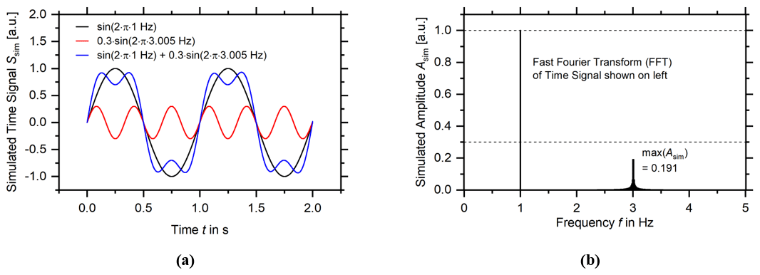
Figure 2(a) An example of a simulated time signal, consisting of two contributions with different amplitudes and frequencies. The full simulated time signal is 100 s long; two periods are shown here. (b) The fast Fourier transform (FFT) of the time signal in panel (a).
Here, a simulated time signal is shown which is exactly 100 s long and contains 220 data points. The signal consists of two contributions, one at 1 Hz which oscillates exactly 100 times during the duration of the time signal and another at 3.005 Hz, which oscillates 300.5 times. As a consequence of the integer number of oscillations, the contribution at 1 Hz is reflected as a single, delta-shaped peak in the FFT shown in Fig. 2b, and as a consequence of the non-integer number of oscillations, the contribution at 3.005 Hz is reflected as a broadened peak. In the case of signal contributions which do not fulfill the requirement that they have an integer number of oscillation periods in the time signal, the height Apeak of the peak can be reconstructed from the region in which it is dominant (i.e., between the minima located closest to the peak on the frequency axis) using
In Eq. (1), i denotes the index of the frequency bin in the FFT. The index iprevious is the position of the minimum closest to the peak at lower frequencies, inext is that of the minimum closest to the peak at higher frequencies, and Ai is the amplitude of the frequency bin with the index i. However, this method is prone to error since it limits itself to the region where the peak dominates the noise and even sums up the noise there. A more accurate detection of amplitudes is achieved by sampling an integer number of periods, as demonstrated here with the 1 Hz sine wave and the corresponding delta peak. Given this fact, Eq. (1) did not need to be applied here and is discussed for the sake of completeness. In the case of a harmonic signal (i.e., a sine wave), only the fundamental mode would be present, and the displacement would be proportional to its amplitude.
The periodicity of the chemical expansion and, thereby, the displacement of the surface require periodic changes of the chemical activity of oxygen in the film, and this is achieved here by electrochemically pumping oxygen from the thin film to the atmosphere and vice versa (see Sect. 3.2). The approach is demonstrated and explained in more detail in Swallow et al. (2017), Wulfmeier et al. (2022), and Kohlmann et al. (2023a, b). Note that for diluted systems, the effective oxygen partial pressure as used below is equivalent to the chemical activity of oxygen in the thin film. The oxygen partial pressure in the vicinity of the sample, i.e., in the furnace, is always 0.21 bar.
Further, pumping of oxygen offers the advantage over other methods of oxygen activity adjustment to virtually arbitrary levels at any speed with exact periodicity due to the periodic setting of the external electrical potential. It eliminates the surface exchange between the surrounding gas and the thin film, which is necessary when the atmosphere is regulated as in, e.g., Kogut et al. (2021, 2022), Schulz et al. (2013), and Sheth et al. (2016). In Guan et al. (2017), the surface gas exchange was found to be the rate-determining step, necessitating equilibration times on the scale of hours, with the effect of the migration of oxygen vacancies across the PCO–YSZ interface being negligible.
1.3 Contradiction to theory motivates a novel approach
A dataset with the displacements of the sample measured at T = 650 and 700 °C for pumping voltages of 0.25, 0.50, and 0.75 V is shown in Fig. 4. Unexpectedly, an increase in pumping voltage leads to an apparent decrease in displacement at low frequencies: the displacements measured with a pumping voltage of 0.75 V are lower than those measured with 0.50 V. If this were to accurately reflect the motion of the sample surface, it would be in direct contradiction to the theory; this allows three conclusions to be drawn:
- 1.
Firstly, the sample is broken, which we have ruled out: the sample is intact and the data consistent.
- 2.
Secondly, the measurement is faulty, which cannot entirely be ruled out but is improbable because the detection is entirely decoupled from the excitation.
- 3.
The third possible conclusion is that measurement and sample are both in order and that the information we seek is contained in the data, but further steps are required to extract it properly. This is the working hypothesis of this paper. It will be shown that this unexpected behavior cannot only be explained by the new evaluation method; it is even mandatory to apply such a sophisticated, multi-step approach to obtain correct results.
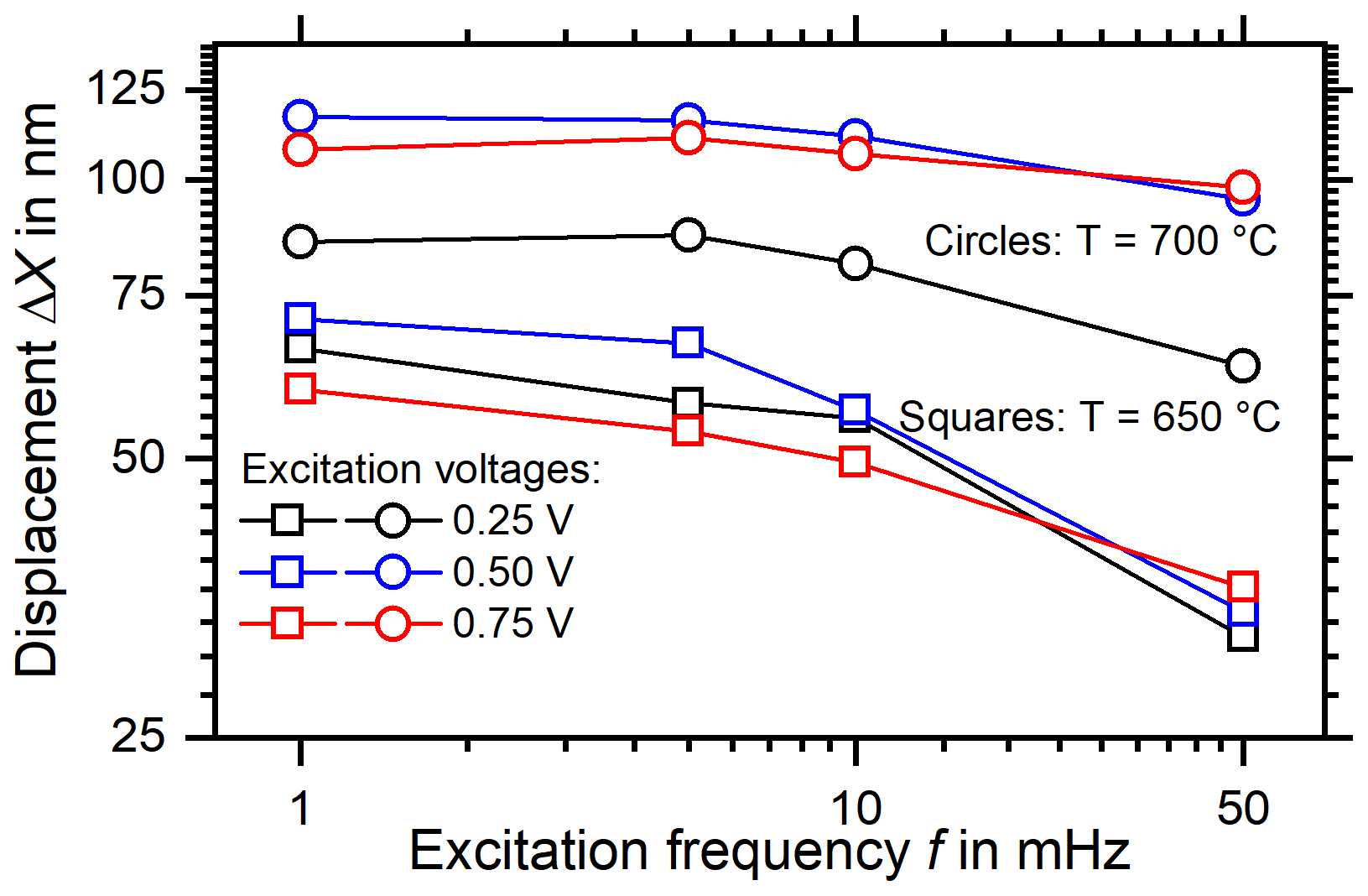
Figure 4The displacements of a PCO thin-film sample, as calculated from the peak at the excitation frequency in the Fourier transform of the time signal. The fact that the displacement values obtained with U = 0.75 V are consistently lower than those with U = 0.50 V constitutes a direct contradiction to theory and motivates a multi-step filtering approach to extract the true displacement from the time signal.
2.1 Oxygen non-stoichiometry and chemical expansion
As illustrated by Fig. 1, the model material PCO exhibits a -dependent oxygen non-stoichiometry δ. The dependence of δ can be separated into three regimes at high, intermediate, and low . In the high region at bar, Pr ions are gradually reduced from their tetravalent state to the trivalent state, excorporating half an oxygen molecule for every two ions reduced (Bishop et al., 2011a). Written in Kröger–Vink notation (Kröger and Vink, 1956), the reaction reads
In Eq. (2), the subscript denotes the lattice site and the superscript the charge relative to the stoichiometric crystal, with a dot representing a positive, a slash a negative, and a cross a neutral charge. The letter V denotes a vacancy. For example, denotes a 2-fold positively charged vacancy occupying an oxygen lattice site. Disregarding impurities and defect interactions and assuming the concentration of oxygen ions to be virtually constant, the relationship between the non-stoichiometry δ, which is proportional to the concentration of vacancies, can be expressed as
which describes the slope of the data curve in the region of high of Fig. 1. In the intermediate region, 10−6 bar bar, all Pr ions in the material are reduced from the tetravalent state to the trivalent state, and the reduction of Ce ions is still negligible. The resulting non-stoichiometry δ is thus constant in this regime. At the transition between these two regimes, the approximations made during the step from Eqs. (2) to (3) no longer hold, and the data curve smoothly turns from a nearly linear increase to constant. In the region of low < 10−16 bar, which is not accessed in the experiments conducted for this work, Ce ions are reduced to the trivalent state.
The change in composition is accompanied by a relative change in lattice parameter called chemical expansion εC, which is in good approximation proportional to the non-stoichiometry δ (Marrocchelli et al., 2012; Bishop et al., 2014) and, therefore, also exhibits a plateau in the same region:
In Eq. (4), a denotes the lattice parameter before expansion, Δa its absolute change, and αC the chemical expansion coefficient. The exact mechanisms linking the non-stoichiometry are the subject of much ongoing research (Schmitt et al., 2020). The most important contributions are steric (the metal ions grow in radius upon accepting an additional electron; Shannon, 1976) and electrostatic (the additional charges repel each other; Marrocchelli et al., 2012).
As εC is proportional to δ, it also exhibits a plateau region at intermediate .
2.2 Mechanical behavior of the sample
The chemical expansion of a thin film deposited on a non-expanding or differently expanding substrate leads to a displacement ΔX of the sample surface, which is the sum of two contributions, the film thickness change Δtf and the substrate-bending Δx. The sample behavior is laid out in Schmidtchen et al. (2018), Wulfmeier et al. (2022), and Kohlmann et al. (2023a, b) and reads
In Eq. (5), tf is the thickness of the thin film, Ef its Young's modulus, and νf its Poisson's ratio. Es, ts, and νs are the Young's modulus, thickness, and Poisson's ratio of the substrate, and r is the radius of the circular sample.
Because ΔX is proportional to εC and therefore to δ (Bishop et al., 2014), it, too, exhibits a plateau in the same region. By driving , one can excite the sample so that its surface is displaced.
2.3 Detection of the displacement
The displacement of the sample, given by Eq. (5), can be detected in several ways. A nanoindenter can be used, which detects the displacement of its tip mechanically (Swallow et al., 2017), or it can be detected interferometrically (Wulfmeier et al., 2022; Kohlmann et al., 2023a, b). The chemical expansion can be measured by thin-film XRD (Sheth et al., 2016) or calculated from the curvature of a wafer (Sheth et al., 2016; Das et al., 2018; Ma and Nicholas, 2018). The displacement can subsequently be calculated from the chemical expansion, and vice versa, using Eq. (5).
While a curvature measurement detects the difference of angle by which two parallel laser beams are deflected when directed at the sample surface and can be obtained as a function of time as in Sheth et al. (2016) and can in principle yield the same information as the LDV experiment, the limiting factor in Sheth et al. (2016) is the surface gas exchange, and the data presented there do not contain information about transport or reaction kinetics.
Thin-film XRD requires the sample to be in a steady state during a lengthy measurement. Thin film therefore does not yield any information about the kinetics of the processes leading to the build-up of the displacement.
The two aforementioned methods, on the other hand, are dynamic: they measure a displacement over time, repeated periodically. This is necessary because the displacement to be measured is overlaid by noise from, e.g., parasitic vibrations, or length fluctuations arising from temperature instabilities. This means that in order to accurately detect the displacement, one must either measure very often and then calculate an average over all periods directly in the time domain or conduct a Fourier transform of the sampled time signal and extract the displacement from the spectrum in the frequency domain (in the following, “in the time domain” specifies that a time signal is being processed and “in the frequency domain” a frequency spectrum). This is of course only possible if the displacement to be detected finds its expression as a sharp, dominant peak which can be clearly discerned from the noise underlying it. The noise level represents the lower detection limit. The displacement is then proportional to the amplitude in the spectrum at the respective frequency. By varying, for example, the amplitude or frequency of the excitation of the sample, one can draw conclusions about how fast the displacement reaches saturation, which contains information about the diffusion and other processes involved, e.g., overpotentials or imperfections in the thin films.
3.1 Sample preparation and parameters
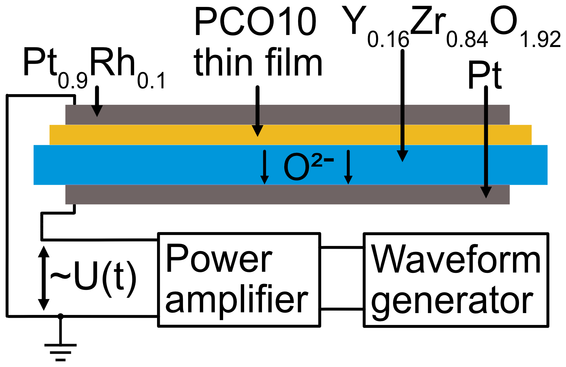
The sample, which is depicted schematically in Fig. 4, is a pumping cell, consisting of four parts: an ionically conducting but electronically insulating single-crystalline Y0.16Zr0.84O2 (8YSZ, MTI Corp., USA) substrate, which acts as a pumping cell (circular, thickness ts= 520 µm, radius r = 5 mm). YSZ is chosen because it is a well-known, readily available, temperature-resistant material which conducts oxygen ions but is electronically insulating. Single-crystal substrates are taken because their mechanical and electrical properties are known and uniform and also because they are electronically insulating, unlike polycrystalline substrates, which might have non-uniform properties strongly deviating from those of the single crystal and might have electronically conducting grain boundaries. The thicknesses of the samples used so far for samples of the type shown in Fig. 3 range from about 200 to about 530 µm. Below 200 µm, the substrate becomes too fragile for the sample preparation process, and above 500 µm, the bending-related displacement becomes small. Additionally, with the substrate being orders of magnitude thicker than the thin film, the pumping voltage applied to the sample drops mainly over the thickness of the substrate, leaving the entire film approximately at uniform potential. Another effect of this discrepancy in thicknesses is the applicability of the Stoney model (Stoney, 1909; Ohring, 1992; Freund and Suresh, 2003), which involves the approximation that the substrate is far thicker than the thin film.
Upon this pumping cell, the PCO thin film is deposited by high-temperature pulsed laser deposition (PLD) as described in Wulfmeier et al. (2022). Upon the film, a Pt0.9Rh0.1 cover electrode is deposited by PLD. On the back side of the substrate, a screen-printed Pt electrode is applied, providing a three-phase boundary between the substrate, the electrode, and the air. The substrate thickness was determined with a thickness gauge (Extramess 2000, MAHR GmbH, Germany), that of the PCO thin film (circular, diameter 9.5 mm, thickness tf = 590 nm) with a stylus profilometer (XP-2, Ambios Technology Inc., USA). The crystallinity of the thin film was confirmed by XRD (D5005, Siemens AG, Germany) and its compactness by SEM (SmartSEM, Carl Zeiss AG, Germany). The characterization of the samples regarding crystallinity, morphology, and density is not shown here, as it is not the main scope of this work and can be found in Chen et al. (2013, 2014), Swallow et al. (2017), Schmidtchen et al. (2018), Wulfmeier et al. (2022), and Kohlmann et al. (2023a, b).
3.2 Excitation of the sample
By applying a negative voltage to the electrode on the PCO thin film depicted in Fig. 3a, oxygen ions are pumped from the thin film into the substrate, from which molecular oxygen is released into the air at the backside electrode. Rearranging the Nernst relation yields the effective oxygen partial pressure in the thin film:
In Eq. (6), is the oxygen partial pressure of the ambient air. The oxygen activity strives toward equilibrium with , which means that oxygen is pumped out of the thin film into the substrate and from the substrate into the air. The effective oxygen partial pressure is equivalent to the chemical activity. With the work laid out in Sect. 2.1, 2.2 and 2.3, it becomes clear that by applying a periodic voltage to the sample (shown schematically in Fig. 2), a periodic deformation is induced. The devices used are a waveform generator (TrueForm 33509b, Keysight Technologies Inc., USA) and a voltage-controlled power amplifier (SVM 02, MST Scientific, Germany) which supplies the pumping current. The pumping voltages specified later on are the high levels of a sine voltage, with the low level always being at 0 V. The negative potential is at the electrode on the PCO thin film, as shown in Fig. 3 (see also Fig. 4 of Wulfmeier et al., 2022).
In Kohlmann et al. (2023b), the displacement of a sample was examined as a function of excitation voltage to determine the value of overpotentials arising from, e.g., contact potentials at interfaces between the different materials, and a value of 0.15 V was found. Considering this value, the effective oxygen partial pressures set in the film are still within the plateau region at pumping potentials U = 0.75 and 0.50 V and outside of it at U = 0.25 V. Thus, the authors' expectation is that even considering overpotentials, when applying sine voltages with a maximum of 0.75 or 0.50 V to the sample, the equilibrium displacements obtained should be equal and larger than that obtained at 0.25 V.
3.3 Measurement setup
The sample is placed in an alumina ceramic holder and contacted with platinum foil. The sample holder is placed inside a tube furnace (LOBA-1200, HTM Reetz GmbH, Germany). When the oxygen is removed and the film expands, the entire sample is bent, shown schematically in Fig. (5a). The full displacement ΔX as the sum of the film thickness change Δtf and the bending Δx is detected by differential laser Doppler vibrometry, as demonstrated in Kohlmann et al. (2023b). By placing the reference beam of the D-LDV on the sample holder, parasitic vibrations, heat haze, sample holder fluctuations, and other disturbances are eliminated to a great degree in the raw signal (Schewe et al., 2023). The adjustment of the beam positions is done with tilt mirrors (Fig. 5b). The interference signal from the D-LDV is decoded with a commercial LDV controller (OFV 5000, Polytec GmbH, Germany) using a DD-500 displacement decoder operated with a range of 50 nm V−1. With the wavelength of 1550 nm of the D-LDV and the controller being designed for a wavelength of 633 nm, the proportionality factor linking the measured voltage to the displacement is 122.47 nm V−1 in the time domain and 244.94 nm V−1 in the frequency domain:
The decoded signal is sampled with an oscilloscope (PCI-5122, National Instruments Corporation, USA) and transferred to a computer for processing and evaluation.
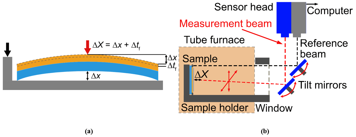
Figure 5(a) Schematic of the contributions to the displacement and its detection. The displacement is the sum of the film thickness change Δtf and the sample bending Δx. The beams are placed on the sample and the sample holder. (b) Schematic of the measurement setup. The sample is placed inside an Al2O3 ceramic holder inside a tube furnace. The two beams of the D-LDV are positioned on the sample and the sample holder, using tilt mirrors. The interference signal is decoded with a commercial LDV controller and sampled with an oscilloscope.
The data treatment to accurately extract the value of the anharmonic displacement of the sample surface will be demonstrated here on a D-LDV measurement conducted on a PCO thin-film sample at T = 650 °C with a pumping voltage of U = 0.75 V at a frequency of f = 0.005 Hz. First, the raw time signal is presented, together with its Fourier transform and the displacement calculated from the fundamental mode alone. In the following steps, a filter is applied to the raw time signal, and the filtered signal Fourier transformed. The spectrum obtained by Fourier transforming the time signal is again filtered, followed by an inverse Fourier transform. The time signal obtained in this way is then read out and the displacement calculated from the peak-to-plateau difference using Eq. (7). At each step, the noise is also extracted, illustrating the decrease of the lower detection limit.
4.1 Displacement signal
The raw displacement time signal of the D-LDV, corrected for these steps as shown in Fig. 6a, still contains considerable noise, as is evident from the drift of over 1.5 µm over the course of 12 h. However, it is orders of magnitude less than that of a single-spot LDV measurement, which is typically over 1 µm in 20 min (Schewe et al., 2023). The absolute value of the Fourier transform (FFT; Harris et al., 2020) of the raw signal is shown in Fig. 6b. The low-frequency f−1 type noise is clearly visible, as are higher harmonics at integer multiples of the excitation frequency 5 mHz, which arise from the periodic but non-harmonic character of the displacement in the time domain. The noise around the peaks is calculated as the rms value of ±20 frequency bins around the excitation frequency in the FFT (±436 µm Hz in this case). The amplitude of the fundamental mode at the excitation frequency is (0.204 ± 0.016) V, which translates to (50.0 ± 3.9) nm using Eq. (7).
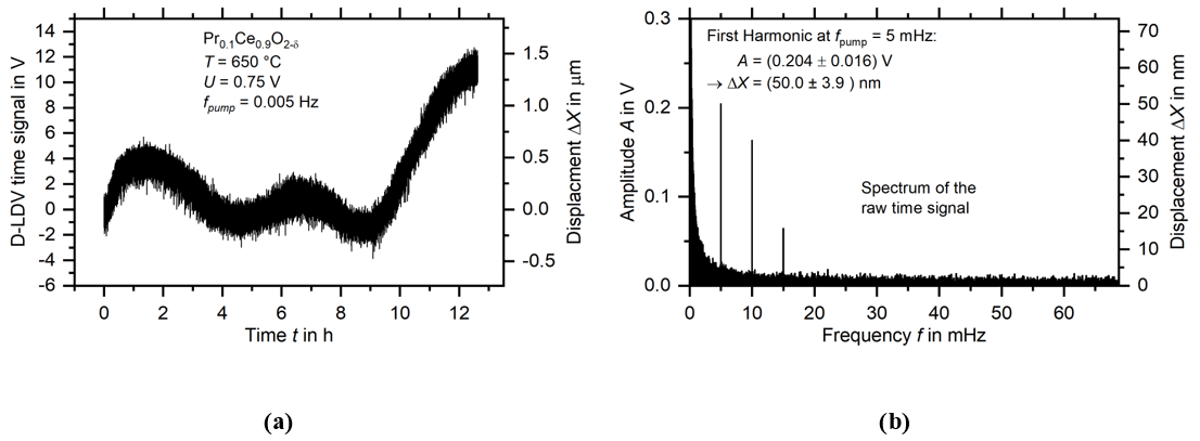
Figure 6(a) The raw displacement time signal of a D-LDV measurement on a PCO thin-film sample at T = 650 °C with pumping voltage U = 0.75 V and excitation frequency f = 0.005 Hz. (b) The Fourier transform of the raw time signal with resolution bandwidth RBW = 22.9 µHz. Higher harmonics at 0.010 and 0.015 Hz are clearly visible.
4.2 First filtering step: time domain filtering
To eliminate the large, low-frequency noise, two steps are taken. First, the time signal is linearly detrended by subtracting a straight line through the first and last points of the portion of the signal which is subsequently used for the FFT. After detrending, a high-pass filter is applied. For the subsequent steps, it is required to be maximally flat in its passband and have a linear phase relation. The first requirement already precludes most filters, e.g., Chebyshev or Bessel, which are not monotonous near their cutoff frequency (Rabiner and Gold, 1975a; Shenoi, 2006), but is met by the Butterworth filter (Virtanen et al., 2020). The second requirement is not met by the Butterworth filter, but this problem can be overcome by implementing it as a sequence of two third-order Butterworth filters, each followed by a reversal of the time axis. The result is that the phase shift from the first Butterworth filter is exactly canceled out by that of the second filter. For this, the cutoff frequency of the third-order filter must be corrected, so that the gain of the third-order filter at the desired cutoff frequency is 1.5 dB, resulting in a dampening of 3 dB at the desired cutoff frequency after applying the filter twice. The over- and undershoots at the beginning and end of the time signal (Rabiner and Gold, 1975a; Shenoi, 2006) are then cut off, making a filter buffer of several excitation periods at both ends necessary. In order not to waste measurement time and expose the sample to harsh conditions for too long, it should be kept short but long enough for the under- and overshoots to be removed by cutting off the buffer. Here, a buffer length of 8 % of the total signal length is chosen, resulting in 8.7 periods at each end for a sixth-order Butterworth high-pass filter with the cutoff frequency half a decade below the excitation frequency. The Butterworth filter thereby fulfills the requirements, albeit at the cost of a longer measurement (in this case half an hour each at both ends of the time signal).
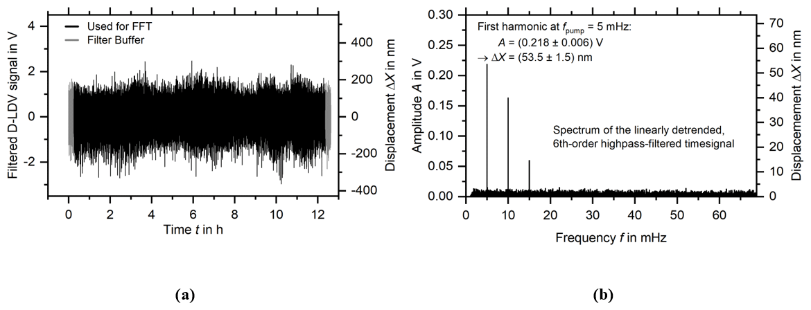
Figure 7(a) The linearly detrended and sixth-order high-pass-filtered time signal. Depicted in grey is the filter buffer, which contains under- and overshoots of the signal and is subsequently cut off. (b) The Fourier transform of the linearly detrended and high-pass-filtered spectrum. The noise level around the first peak at the excitation frequency is reduced by around 60 %.
In Fig. 7a, the filtered time signal is shown, with the filter buffer, which will subsequently be discarded, shown in grey. In Fig. 7b, the Fourier transform of the high-pass-filtered time signal is shown, with the fundamental mode and the second and third harmonics clearly visible. Direct comparison with the spectrum of the unfiltered time signal in Fig. 6b shows that the noise around the fundamental mode, which represents the lower detection limit of the D-LDV (or any other measurement technique), has been reduced by almost 60 % from ±0.016 V, corresponding to ±3.9 nm, down to ±0.006 V, which corresponds to ±1.5 nm. The height of the fundamental mode is increased by 7 % from 0.204 V, corresponding to 50.0 nm, to 0.218 V, corresponding to 53.5 nm. The signal-to-noise ratio (SNR) is consequently increased from 12.8 without the filter to 35.9 after the application of the high-pass filter.
4.3 Second filtering step: frequency domain filtering
In the next step, the signal is filtered in the frequency domain, meaning that the spectrum shown in Fig. 7b is used. First, the signal-to-noise ratio (SNR) is calculated for each harmonic, with the noise level again being taken as the rms value of the 40 FFT bins closest to the harmonic. All harmonics with SNR < 1.5 are discarded. When 10 harmonics have been discarded using this criterion, the process is ended, and no higher harmonics are considered anymore. Next, the delta shape of the peaks at the integer multiples of the excitation frequency is exploited. As shown schematically in Fig. 2, the Fourier transform of a periodic time signal consists of delta-shaped peaks at the fundamental mode and the higher harmonics, i.e., the integer multiples of the fundamental frequency. Consequently, all in between harmonics is considered noise and discarded, leaving a spectrum consisting only of a few delta-shaped peaks at integer multiples of the excitation frequency, as shown in Fig. 8.
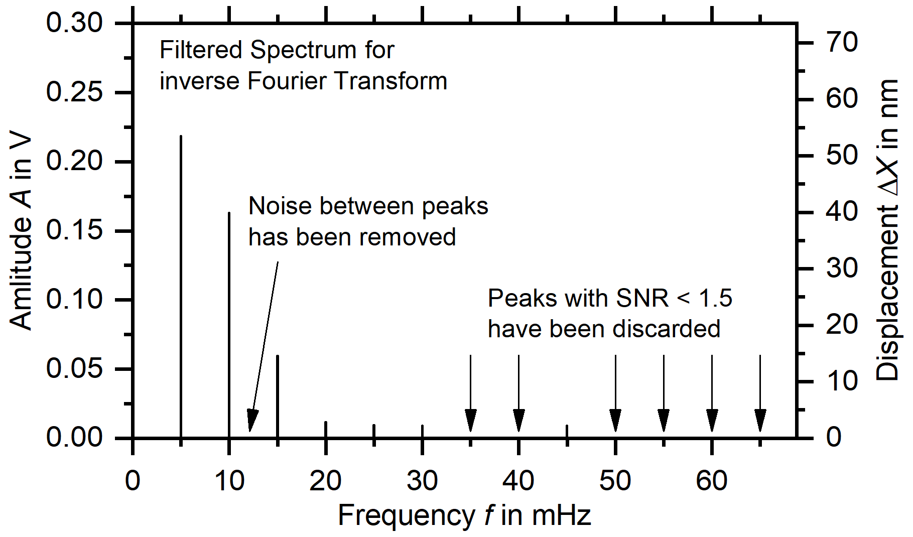
Figure 8The filtered spectrum, consisting of contributions at higher harmonic frequencies with an SNR > 1.5 only.
4.4 Back transformation and readout of recovered signal
The filtered spectrum shown in Fig. 8 is then transformed back into a time signal with an inverse Fourier transformation (iFFT; Harris et al., 2020), and two periods are saved as a resulting dataset to be read out (shown in Fig. 9), as all periods of the time signal are identical. The minimum is extracted from the dataset and the plateau taken as the average between the first and last maximum of the time signal, with the uncertainty being the standard deviation of this region. In the case of the measurement taken here to demonstrate the approach, the displacement obtained this way of 69.4 nm is ca. 38 % larger than that calculated from the peak at the first harmonic only. The standard deviation of the plateau of 2.6 nm is ca. 34 % smaller than the noise level of the raw spectrum shown in Fig. 6b, which was taken as the uncertainty.
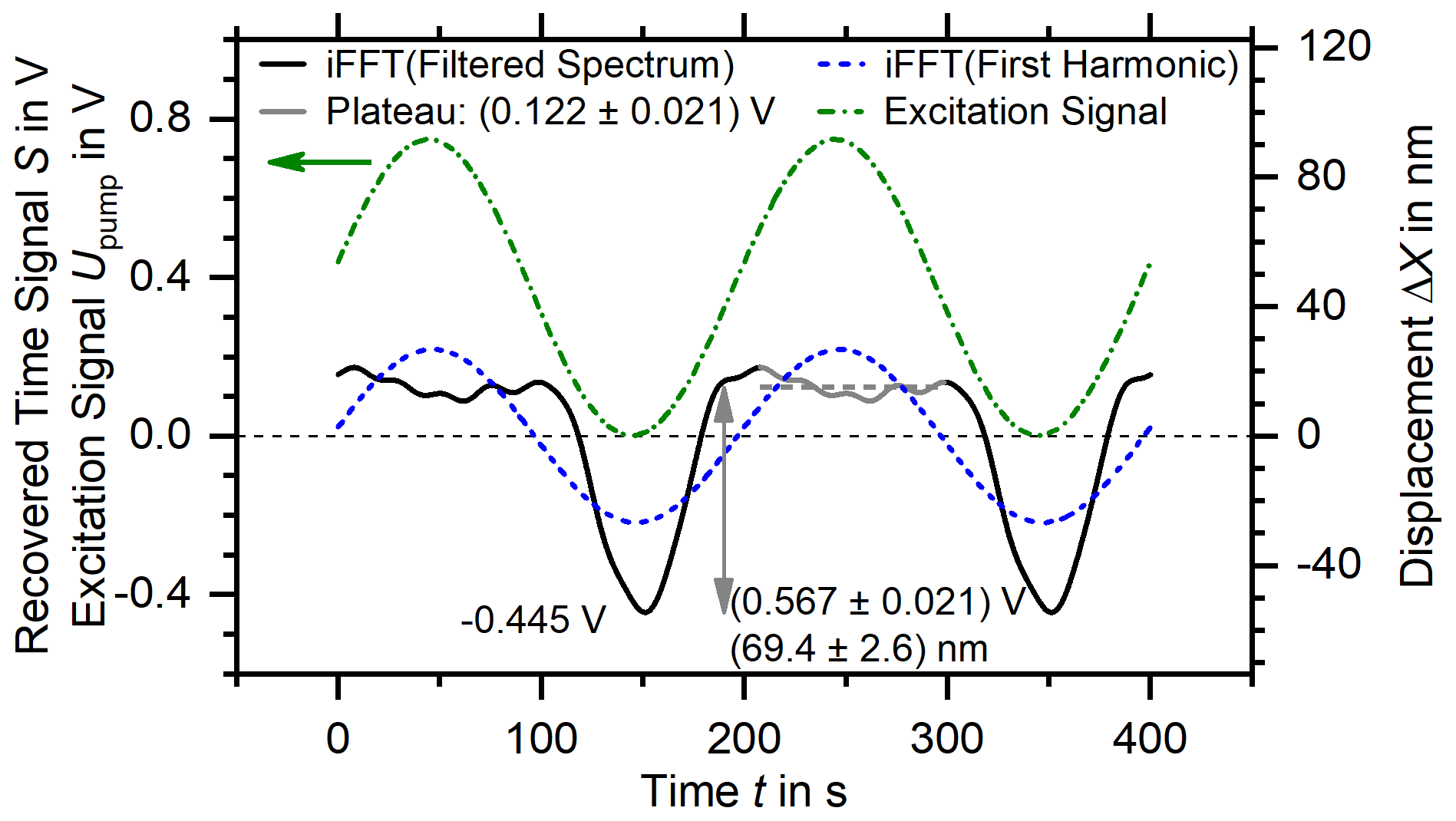
Figure 9The backtransformed time signal (iFFT; Harris et al., 2020) generated from the spectrum in Fig. 8. The excitation signal shown in green belongs to the left ordinate only, while all other graphs belong to both ordinates. The total displacement is proportional to the difference between the minimum and the constant displacement region marked in gray, taken as the region between the first and last maximum. For comparison, the iFFT of the spectrum consisting of only the peak at the excitation frequency is shown as a dashed blue line.
4.5 Comparison with evaluation of first harmonic only
In Fig. 10, the displacements obtained with this method from the same measurements as in Fig. 3 are shown and compared to those calculated directly from the peak at the first harmonic. The contradiction to the theory, which motivated this new approach, has been resolved, which is apparent in that an increase in pumping voltage no longer leads to a decrease in displacement within the margin of uncertainty. The displacement increases monotonously with increasing pumping voltage, with almost equal displacements at pumping voltages 0.50 and 0.75 V, which indicates that non-linear reactions of the sample upon the excitation can now be detected accurately, validating our approach. The plateau of the non-stoichiometry shown in Fig. 1 is reflected in the constant displacement directly visible in the backtransformed time signal in Fig. 9.
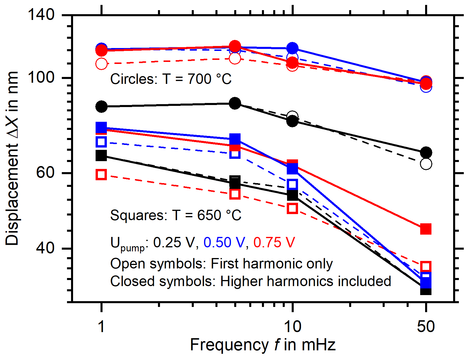
Figure 10The displacements of the sample at T = 650 and 700 °C, measured with pumping voltages U = 0.25, 0.50, and 0.75 V at frequencies f = 1, 5, 10, and 50 mHz.
With the new approach to the evaluation of D-LDV data, extremely small, very slow movements in harsh, noisy conditions as in high-temperature furnaces, or chemical reactors, can now be directly observed. Non-linear displacements can be determined more accurately: in the case of the dataset processed here, the displacement extracted directly from the Fourier spectrum of the raw time signal is (50.3 ± 3.9) nm, while the displacement extracted with the method presented here is (69.4 ± 2.6) nm, which constitutes an increase in the detected displacement of 38 %, while the uncertainty is reduced by 33 %. The increase in displacement is confirmed by the fact that an increase in pumping voltage leads to an increase in displacement or a constant displacement for pumping voltages in the plateau region as shown in Fig. 1 but no longer leads to a decrease in detected displacement. Displacements on the order of single nanometers are discernible in noisy environments like high-temperature furnaces at frequencies down to 1 mHz, with the noise level at 1 mHz and 650 °C being 1.5 nm. As with all contactless measurement methods, there is no influence of the measurement on the sample. The method could, with adjustments, be used to detect very small optical and electrical signals, or anharmonic contributions and higher-order, non-linear effects to otherwise linear physical effects. Applied to piezoelectric crystals, e.g., lithium tantalate (LT; LiTaO3), lithium niobate (LN; LiNbO3), or their solid solutions lithium niobate–tantalate (LNT; LiNbxTa1−xO3), it could allow for the determination of higher-order contributions to piezoelectricity and for the very precise determination of piezoelectric constants and, subsequently, mechanical properties of piezoelectric crystals and materials deposited thereon.
The data presented in this article are stored in an internal system according to the guidelines of the German Research Foundation (Deutsche Forschungsgemeinschaft; DFG). Research data are available upon request to the authors.
Funding was equally acquired by HF and CR, who also equally provided for the resources and contributed to conceptualization, the administration, and the supervision of the project. The measurement device is the result of the doctoral project of MS and DK, who provided much of the investigative work for its understanding. All authors contributed equally to the methodology. The investigation was performed by DK, who conducted the experiments and evaluated, curated, and validated the data with MS and HW. The results were validated by CR and HF. The software was built by DK in cooperation with HW, with validations and consistency checks provided and performed by MS. Data were visualized by DK, HW, and HF. All authors contributed equally to the writing of the original draft and the review and editing.
The contact author has declared that none of the authors has any competing interests.
Publisher’s note: Copernicus Publications remains neutral with regard to jurisdictional claims made in the text, published maps, institutional affiliations, or any other geographical representation in this paper. While Copernicus Publications makes every effort to include appropriate place names, the final responsibility lies with the authors.
This article is part of the special issue “Sensors and Measurement Science International SMSI 2023”. It is a result of the 2023 Sensor and Measurement Science International (SMSI) Conference, Nuremberg, Germany, 8–11 May 2023.
The authors are grateful to Harry L. Tuller for valuable discussions and to Thomas Defferriere for preparation of some films used (both Massachusetts Institute of Technology). In addition, the authors thank the Energy Research Centre of Lower Saxony (Energie-Forschungszentrum Niedersachsen; EFZN) for supporting this work.
This research has been supported by the Deutsche Forschungsgemeinschaft (grant nos. FR 1301/31-1, FR 1301/42-1, and RE3980/3-1).
This open-access publication was funded by Clausthal University of Technology.
This paper was edited by Daniel Platz and reviewed by two anonymous referees.
Atkinson, A.: Chapter 2 - Solid Oxide Fuel Cell Electrolytes – Factors Influencing Lifetime, in: Solid Oxide Fuel Cell Lifetime and Reliability, edited by: Brandon, N. P., Ruiz-Trejo, E., and Boldron P., Academic Press, 19–35, https://doi.org/10.1016/B978-0-08-101102-7.00002-7, 2017.
Bishop, S. R.: Chemical expansion of solid oxide fuel cell materials: A brief overview, Acta Mech. Sin., 29, 312–317, https://doi.org/10.1007/s10409-013-0045-y, 2013.
Bishop, S. R., Tuller, H. L., Kuru, Y., and Yildiz, B.: Chemical expansion of nonstoichiometric Pr0.1Ce0.9O2−δ: Correlation with defect equilibrium model, J. Eur. Ceram. Soc., 31, 2351–2356, https://doi.org/10.1016/j.jeurceramsoc.2011.05.034, 2011a.
Bishop, S. R., Stefanik, T. S., and Tuller, H. L.: Electrical conductivity and defect equilibria of Pr0.1Ce0.9O2−δ, Phys. Chem. Chem. Phys., 13, 10165–10173, https://doi.org/10.1039/c0cp02920c, 2011b.
Bishop, S. R., Marrocchelli, D., Chatzichristodoulou, C., Perry, N. H., Mogensen, M. B., Tuller, H. L., and Wachsman, E. D.: Chemical Expansion: Implications for Electrochemical Energy Storage and Conversion Devices, Ann. Rev. Mater. Res., 44, 205–239, https://doi.org/10.1146/annurev-matsci-070813-113329, 2014.
Chen, D., Bishop, S. R., and Tuller, H. L.: Non-stoichiometry in Oxide Thin Films: A Chemical Capacitance Study of the Praseodymium-Cerium Oxide System, Adv. Funct. Mater., 23, 2168–2174, https://doi.org/10.1002/adfm.201202104, 2013.
Chen, D., Bishop, S. R., and Tuller, H. L.: Nonstoichiometry in Oxide Thin Films Operating under Anodic Conditions: A Chemical Capacitance Study of the Praseodymium-Cerium Oxide System, ECS Transactions, 57, 1387, https://doi.org/10.1149/05701.1387ecst, 2014.
Das, T., Nicholas, J. D., Sheldon, B. W., and Qi, Y.: Anisotropic chemical strain in cubic ceria due to oxygen-vacancy-induced elastic dipoles, Phys. Chem. Chem. Phys., 20, 15293–15299, https://doi.org/10.1039/C8CP01219A, 2018.
Freund, L. B. and Suresh, S. (Eds.): Chapter 2: Film stress and substrate curvature, in: Thin Film Materials: Stress, Defect Formation and Surface Evolution, Cambridge University Press, 86–153, https://doi.org/10.1017/CBO9780511754715, 2003.
Guan, Z., Chen, D., and Chueh, W. C.: Analyzing the dependence of oxygen incorporation current density on overpotential and oxygen partial pressure in mixed conducting oxide electrodes, Phys. Chem Chem. Phys., 19, 23414–23424, https://doi.org/10.1039/c7cp03654j, 2017.
Hara, N. C. and Ford, E. B.: Statistical Methods for Exoplanet Detection with Radial Velocities, Annu. Rev. Stat. Appl., 10, 623–649, https://doi.org/10.1146/annurev-statistics-033021-012225, 2023.
Harris, C. R., Millman, K. J., van der Walt, S. J., Gommers, R., Virtanen, P., Cournapeau, D., Wieser, E., Taylor, J., Berg, S., Smith, N. J., Kern, R., Picus, M., Hoyer, S., van Kerkwijk, M. H., Brett, M., Haldane, A., del Río, J. F., Wiebe, M., Peterson, P., Gérard-Marchant, P., Sheppard, K., Reddy, T., Weckesser, W., Abbasi, H., Gohlke, C., and Oliphant, T. E.: Array programming with NumPy, Nature, 585, 357–362, https://doi.org/10.1038/s41586-020-2649-2, 2020.
Klippel, W.: Loudspeaker Nonlinearities – Causes, Parameters, Symptoms, J. Audio Eng. Soc., 119, 907–939, 2005.
Kogut, I., Steiner, C., Wulfmeier, H., Wollbrink, A. Hagen, G., Moos, R., and Fritze, H.: Comparison of the electrical conductivity of bulk and film Ce1−xZrxO2−δ in oxygen-depleted atmospheres at high temperatures, J. Mater. Sci., 56, 17191–17204, https://doi.org/10.1007/s10853-021-06348-5, 2021.
Kogut, I. , Wollbrink, A., Steiner, C., Wulfmeier, H., El Azzouzi, F. E., Moos, R., and Fritze, H:. Linking the Electrical Conductivity and Non-Stoichiometry of Thin Film Ce1−xZrxO2−δ by a Resonant Nanobalance Approach, Materials, 14, 748, https://doi.org/10.3390/ma14040748, 2022.
Kohlmann, D., Schewe, M., Kogut, I., Steiner, C., Moos, R., Rembe, C., and Fritze, H: Chemical expansion of CeO2−δ and Ce0.8Zr0.2O2−δ thin films determined by Laser Doppler Vibrometry at high temperatures and different oxygen partial pressures, J. Mater. Sci., 58, 1481–1504, https://doi.org/10.1007/s10853-022-07830-4, 2023a.
Kohlmann, D., Schewe, M., Wulfmeier, H., Defferriere, T., Rembe, C., Tuller, H. L., and Fritze, H.: High-temperature chemical expansion of Pr0.1Ce0.9O2−δ thin films determined by Differential Laser Doppler Vibrometry, Solid State Ionics, 392, 116151, https://doi.org/10.1016/j.ssi.2023.116151, 2023b.
Kröger, F. A. and Vink, H. J.: Relations between Concentrations of Imperfections in Crystalline Solids, Solid State Phys., 3, 307–435, https://doi.org/10.1016/S0081-1947(08)60135-6, 1956.
Ma, Y. and Nicholas, J. D.: Mechanical, thermal, and electrochemical properties of Pr doped ceria from wafer curvature measurements, Phys. Chem. Chem. Phys., 20, 27350–27360, https://doi.org/10.1039/C8CP04802A, 2018.
Marrocchelli, D., Bishop, S. R., Tuller, H. L., and Yildiz, B.: Understanding Chemical Expansion in Non-Stoichiometric Oxides: Ceria and Zirconia Case Studies, Adv. Funct. Mater., 22, 1958–1965, https://doi.org/10.1002/adfm.201102648, 2012.
Ohring, M.: Chapter 9.3: Internal Stresses and Their Analysis, in: Materials Science of Thin Films, Internal Stresses and their analysis, Academic Press, 413–420, https://doi.org/10.1016/C2009-0-22199-4, 1992.
Preux, N., Rolle, A., and Vannier, R. N.: Chapter 12: Electrolytes and ion conductors for solid oxide fuel cells (SOFCs), in: Functional materials for sustainable energy applications, edited by: Kilner, J., Kinner, S., Irvine, S., and Edwards, P., Woodhead Publishing Ltd., 370–394, https://doi.org/10.1533/9780857096371.3.370, 2012.
Rabiner, L. R. and Gold, B.: Chapter 4: Theory and Approximation of Infinite Response Digital Filters, in: Theory and Application of Digital Signal Processing, Prentice-Hall, 205–294, ISBN 0-13-914101-4, 1975a.
Rabiner, L. R. and Gold, B.: Chapter 6: Spectrum Analysis and the Fast Fourier Transform, in: Theory and Application of Digital Signal Processing, Prentice-Hall, 356–437, ISBN 0-13-914101-4, 1975b.
Schewe, M., Rembe, C., Fritze, H., Wulfmeier, H., and Kohlmann, D.: Differential laser Doppler vibrometry for displacement measurements down to 1 mHz with amplitude resolution below 1 nm, Measurement, 210, 112576, https://doi.org/10.1016/j.measurement.2023.112576, 2023.
Schmidtchen, S., Fritze, H., Bishop, S. R., Chen, D., and Tuller, H. L.: Chemical expansion of praseodymium-cerium oxide films at high temperatures by laser doppler vibrometry, Solid State Ionics, 319, 61–67, https://doi.org/10.1016/j.ssi.2018.01.033, 2018.
Schmitt, R., Nenning, A., Kraynis, O., Korobko, R., Frenkel, A. I., Lubomirsky, I., Haile, S. M., and Rupp, J. L. M.: A review of defect structure and chemistry in ceria and its solid solutions, Chem. Soc. Rev., 49, 554–592, https://doi.org/10.1039/C9CS00588A, 2020.
Schulz, M., Fritze, H., and Stenzel, C.: Measurement and control of oxygen partial pressure at elevated temperatures, Sensor. Actuat. B-Chem., 187, 503–508, https://doi.org/10.1016/j.snb.2013.02.115, 2013.
Shannon, R. D.: Revised Effective Ionic Radii and Systematic Studies of Interatomie Distances in Halides and Chaleogenides, Acta Crystallogr. A, 32, 751–767, https://doi.org/10.1107/S0567739476001551, 1976.
Shenoi, B. A. (Ed.): Infinite Impulse Response Filters, in: Introduction to digital signal processing and filter design, Chap. 4, 186–248, John Wiley & Sons, https://doi.org/10.1002/0471656372.ch4, 2006.
Sheth, J., Chen, D., Kim, J. J., Bowman, P. J., Crozier, P. A., Tuller, H. L., Misture, S. T., Zdzieszynski, S., Sheldon, B. W., and Bishop, S. R.: Coupling of strain, stress, and oxygen non-stoichiometry in thin film Pr0.1Ce0.9O2−δ, Nanoscale, 8, 16499–16510, https://doi.org/10.1039/C6NR04083G, 2016.
Stoney, G. G.: The tension of metallic films deposited by electrolysis, P. Roy. Soc. Lond. A Mat., 82, 172–175, https://doi.org/10.1098/rspa.1909.0021, 1909.
Swallow, J. G., Kim, J. J., Maloney, J. M., Chen, D., Smith, J. F., Bishop, S. R., Tuller, H. L., and Van Vliet, K. J.: Dynamic chemical expansion of thin-film non-stoichiometric oxides at extreme temperatures, Nat. Mater., 16, 749–754, https://doi.org/10.1038/nmat4898, 2017.
Virtanen, P., Gommers, R., Oliphant, T. E., Haberland, M., Reddy, T., Cournapeau, D., Burovski, E., Peterson, P., Weckesser, W., Bright, J., van der Walt, S. J., Brett, M., Wilson, J., Millman, K. J., Mayorov, N., Nelson, A. R. J., Jones, E., Kern, R., Larson, E., Carey, C. J., Polat, İ., Feng, Y., Moore, Eric W., VanderPlas, J., and SciPy 1.0 Contributors: SciPy 1.0: fundamental algorithms for scientific computing in Python, Nat. Methods, 17, 261–272, https://doi.org/10.1038/s41592-020-0772-5, 2020.
Wulfmeier, H., Kohlmann, D., Defferriere, T., Steiner, C., Moos, R., Tuller, H. L., and Fritze, H.: Thin-film chemical expansion of ceria based solid solutions: laser vibrometry study, Zeitschrift für Physikalische Chemie, 263, 1013–1053, https://doi.org/10.1515/zpch-2021-3125, 2022.
- Abstract
- Introduction and motivation
- State of research
- Experimental procedure/materials and methods
- Data treatment and results
- Conclusions and outlook
- Data availability
- Author contributions
- Competing interests
- Disclaimer
- Special issue statement
- Acknowledgements
- Financial support
- Review statement
- References