Efficient hardware implementation of interpretable machine learning based on deep neural network representations for sensor data processing

With the rising number of machine learning and deep learning applications, the demand for implementation of those algorithms near the sensors has grown rapidly to allow efficient edge computing. Especially in sensor-based tasks like predictive maintenance and smart condition monitoring, the goal is to implement the algorithms near the data acquisition system to avoid unnecessary energy consumption caused by extensive transfer of raw data. Deep learning algorithms achieved good results in various fields of application and often allow the efficient implementation on dedicated hardware and common AI accelerators like graphic and neural processing units. However, they often need more interpretability to analyze upcoming results. For this purpose, this paper presents an approach to represent trained interpretable machine learning algorithms, consisting of a stack of feature extraction, feature selection, and classification/regression algorithms, as deep neural networks. This representation retains the interpretability but allows efficient implementation on hardware to process the acquired data directly on the sensor node. The representation is based on dissembling the inference of the trained interpretable algorithm into the basic mathematical operations to represent them with deep neural network layers. The technique to convert the trained interpretable machine learning algorithms is described in detail and applied to parts of an open-source machine learning toolbox. The accuracy, runtime, and memory requirements are investigated on four datasets, implemented on resource-limited edge hardware. The deep neural network representation reduced the runtime compared to a common Python implementation by up to 99.3 % while retaining the accuracy. Finally, a quantization method was successfully applied to interpretable machine learning algorithms, gained an additional reduction of 64.8 % in runtime, and reduced the memory requirement up to 75.6 % compared to the full precision implementation.

1 Introduction

In recent years, the number of machine-learning (ML)-based applications in scientific, medical, and industrial environments has increased considerably. Most of these algorithms try to predict a specific target value, for example, upcoming failures of a monitored machine to prevent downtimes (Mobley, 2002). ML-based applications typically rely on a vast amount of data recorded by different sensors located on or near the monitored machine or application (Hermansa et al., 2021). Transferring the recorded raw data to central instances with high computational power, memory, and energy availability is highly inefficient and represents the most dominant part in the total amount of energy consumption (Muhoza et al., 2023). Some studies try optimizing these processes regarding energy consumption (Ang et al., 2017). However, to avoid this step of raw data transfer, the focus shifted to processing the raw data to complete the ML workflow directly on the recording sensors (Merenda et al., 2020; Pioli et al., 2024). These smart sensors allow the entire workflow, from data recording to data processing, to complete ML applications on the same board (Singh and Gill, 2023). However, most sensors and recording hardware are lacking in terms of computational power and memory requirements. Data processing or the entire ML workflow must be efficient regarding computational time, memory requirements, and energy consumption to allow edge computing solutions. Several articles in the literature examine the use of ML applications in smart sensors and edge hardware (Molinara et al., 2021; Soro, 2021).

ML-based applications can be divided into two areas. On the one hand, there is the area of deep learning (DL), which solves the problem with deep neural networks (DNNs) (LeCun et al., 2015). On the other hand, the field of “classical” ML (Ezugwu et al., 2024) employs a variety of steps such as feature extraction (FE), feature selection (FS), and classification or regression (C/R) algorithms to develop solutions for a given problem. The DNNs, mainly used in DL, are highly effective in detecting complex non-linear relationships between input data and targets. However, these correlations are rarely interpretable. Such “black box” systems do not provide the possibility to interpret the prediction regarding the underlying features and characteristics of the input data (Buhrmester et al., 2021).

Training a DNN requires a large amount of labeled data, which is only sometimes available, especially in industrial ML applications. Due to the need for better explainability, interpretable ML applications consisting of FE, FS, and C/R have gained attention (Goodarzi et al., 2022; Schneider et al., 2018b). This ML approach allows the interpretation of the input data through the different data processing steps. This enables deep feature engineering and the physical analysis of input data characteristics. The ML Toolbox (ZeMA-gGmbh, 2017) is a framework for this approach, which provides various FE, FS, and C/R algorithms (FESC/R). Most of the FESC/R algorithms lack in the implementation on efficient hardware, which is compared in Nguyen et al. (2019). Previous studies have focused on efficient programming by mapping parts of interpretable ML algorithms as matrix multiplications to accelerate the ML inference on hardware optimized for these operations (Pan and Mishra, 2022). Another approach is to design and program specialized hardware, such as ASICs or FPGAs, for efficient implementation of algorithms, which results in high-effort and non-configurable hardware solutions (Neshatpour et al., 2015; Nguyen et al., 2016). On the other hand, the most efficient and generic AI hardware, like graphical processing units (GPUs), neural processing units (NPUs), and tensor processing units (TPUs), can infer DNNs with minimal programming effort. This generic AI hardware allows efficient implementation of ML algorithms regarding runtime, power, or memory usage (Ghimire et al., 2022).

To optimize the inference of interpretable ML algorithms, this paper demonstrates an approach to represent interpretable ML algorithm inference with DNNs for an efficient implementation on resource-limited hardware and a further acceleration on optimized edge hardware without the need for specialized hardware with high-effort access. This allows the best of both worlds, i.e., efficient hardware implementation of DNNs while preserving the interpretability of the ML algorithms. The approach breaks down interpretable ML inferences into basic mathematical operations to represent them as DNN layers. Additionally, the resulting model format and the available parameters and metrics provide a solid approach for estimating hardware requirements regarding computational cost, memory usage, and runtime (Jawandhiya, 2018). Furthermore, the method allows the usage of standard techniques such as quantization (Choukroun et al., 2019; Nagel et al., 2021) to further improve these characteristics. The study focuses on the critical parameters for computing on dedicated hardware. The most important metric is the algorithm's accuracy, which defines the functionality of the ML model. Runtime is a crucial factor in terms of real-time application and energy efficiency. The last parameter studied is memory requirement, which must be highlighted if a limited hardware implementation is desired. The paper presents a representation to optimize memory requirements and runtime of ML algorithms with minimal error, significantly extending the previous conference contributions (Schauer et al., 2024a, b).

The rest of the paper is structured as follows: Sect. 2 describes the materials, metrics, and datasets used for benchmarking the interpretable ML algorithm. Section 3 presents a detailed description of the method for representing the trained interpretable ML algorithm with DNNs. Section 4 presents the results of applying the DNN method to parts of the open-source ML Toolbox. Section 5 discusses the results of the significant reduction in terms of runtime and memory requirement and the accuracy regarding quantization. Finally, Sect. 6 concludes the paper and gives an outlook on future work.

2 Material and methods

This paper focuses on converting trained interpretable FESC/R algorithm stacks to DNN to implement them efficiently on smart sensors and limited edge hardware. The trained models based on the FESC/R algorithm are mathematically interpretable and represent a static equation to calculate the output. The idea is to break down the static equation of the trained model inference into the basic mathematical operations. To optimize the inference of the trained model, which is usually programmed in MATLAB, Python, or C/C$++$, the mathematical operations are replaced by generic neural network layers. Besides layers with specific functions (ONNX, 2023), like average pooling and maximum pooling, a fully connected layer allows the implementation of every mathematical operation executable through matrix multiplications. This enables the implementation of a wide range of different AI and signal-processing algorithms. Those DNN representations benefit from optimized inference and access to common AI accelerators, like GPUs, NPUs, or TPUs, without any further programming effort. This method combines the benefits of interpretable ML and the widespread use of DNN frameworks for optimized inference and hardware implementation.

However, an appropriate FESC/R algorithm must be identified and trained before generating a DNN representation of the model. Figure 1 illustrates the suggested workflow from creating FESC/R algorithms, training, model validation, and representation as a DNN to implementing in a real-world application, for example, condition monitoring (CM) or predictive maintenance (PM). This flowchart represents a common approach and workflow of collaboration between research and developing new algorithms and their efficient usage on sensors in real-world applications. The following section describes the underlying FESC/R Toolbox, the metrics, and the datasets of the later performed benchmarks.

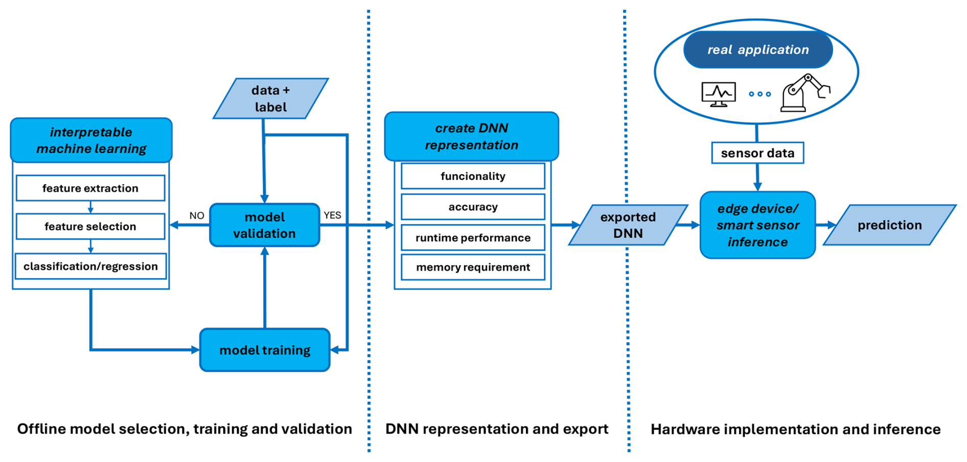
Figure 1 Overview from sensor data acquisition, over deep neural network representation, to hardware implementation and sensor data processing.

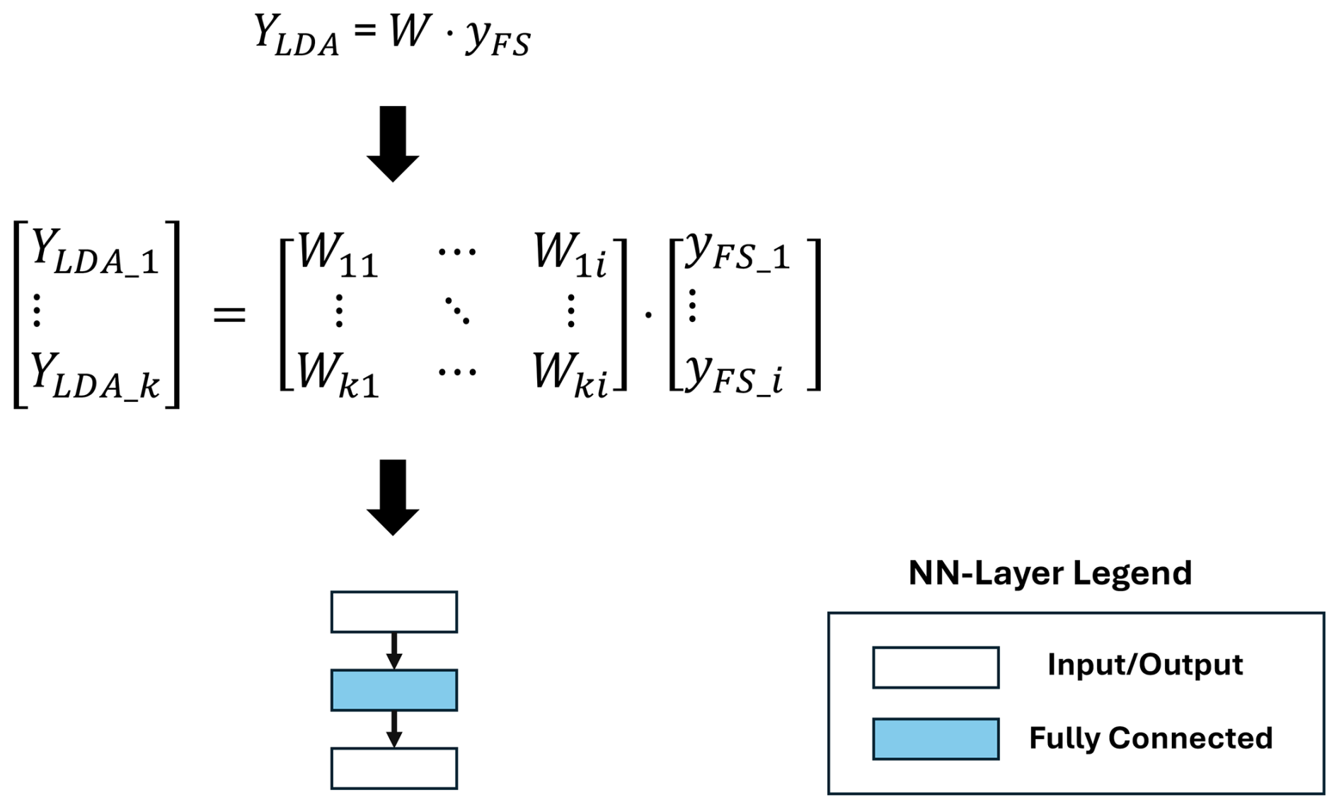
2.1 FESC/R Toolbox

To demonstrate the novel approach of representing trained FESC/R algorithms as DNNs, the methods from the open-source FESC/R Toolbox (ZeMA-gGmbh, 2017) are selected and trained in advance. The FESC/R Toolbox provides complementary methods, allowing users to explore various domain signal representations. The open-source ML Toolbox provides the functionality to develop and train interpretable FESC/R algorithms automatically. Therefore, the toolbox compares the results of combinations of several FS, FE, and C/R algorithms included in the toolbox and chooses the best available algorithm for the specific dataset. This open-source toolbox forms the foundation of the novel approach that can be represented as DNNs after the final model selection. The implemented methods of the toolbox are listed in Table 1, and the three different processing steps are shortly described; the detailed description can be found in Sect. 3.

Table 1 Overview of the feature selection, feature extraction, classification, and regression algorithms of the AutoML Toolbox implemented as deep neural networks.

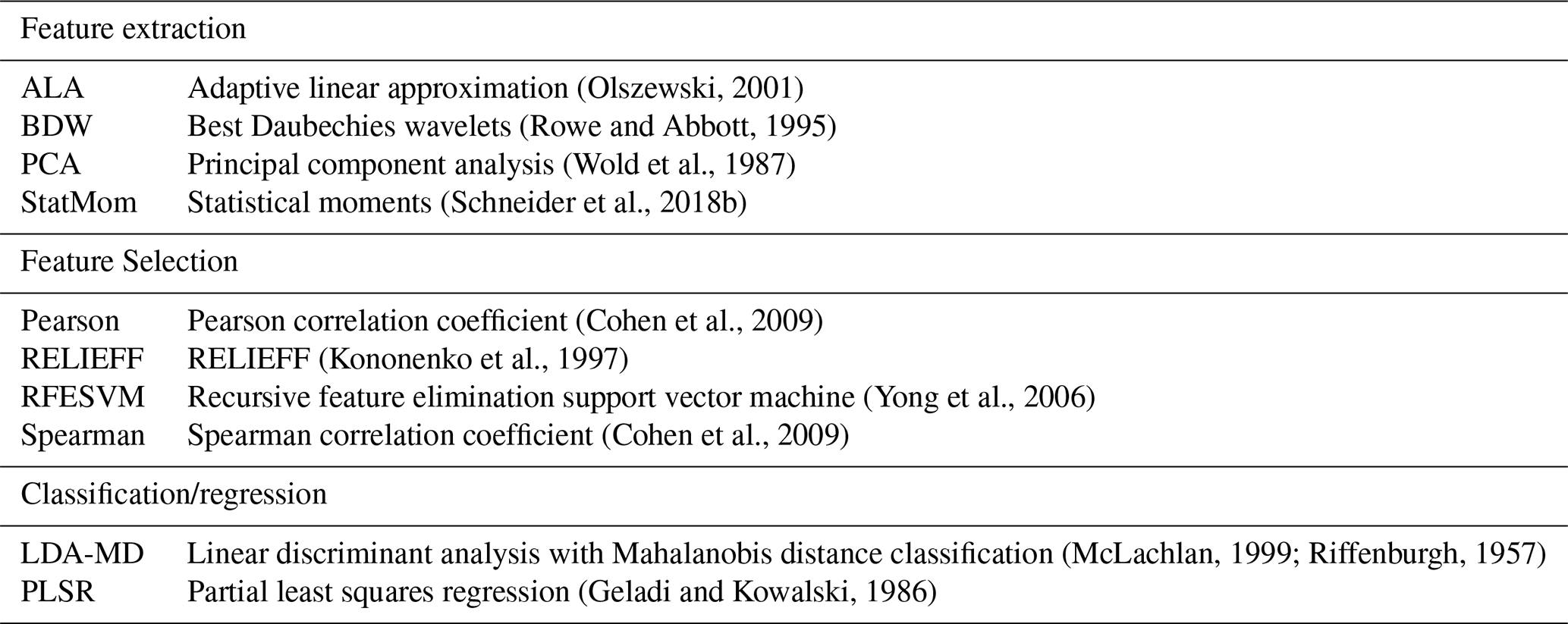
2.1.1 Feature extraction

The FE algorithms try to reduce the dimension by extracting physically interpretable features of the input data. Each FE algorithm calculates different features from various domains, allowing the developer to use the physical or systematical prior knowledge to extract useful features. Representing and reducing input data involves a trade-off between approximation error and the number of features. The goal is to minimize both the approximation error and the number of features. On the one hand, some of the FE algorithms find optimal segmentations and parameters within a previous training process; on the other hand, some of these methods are also not learnable and can be applied without training. In this study, methods that extract features in the time and frequency domains are represented as DNNs.

2.1.2 Feature selection

The FS methods are a supervised part of the FESC/R Toolbox that tries to learn the most significant features extracted by the previously executed FE. The FS methods create a ranking of the informational value of the extracted features and allow the user to reduce the amount of data with minimal loss of information.

2.1.3 Classification and regression

The last element of the FESC/R pipeline is a classifier or a regression algorithm, which calculates the FESC/R output and is also a supervised trainable workflow element. Classifiers try to map the given input to the desired categorical output with a minimal error rate. In contrast, a regression algorithm tries to predict continuous values as an output, e.g., with a minimal root mean square error (RMSE).

2.2 Quantization

An appropriate way to prepare DNNs for fast and energy-efficient hardware implementation is the quantization process. With the DNN representation of interpretable ML algorithms, improving the efficiency of the hardware implementations of interpretable ML algorithms with quantization is possible. DNN quantization describes a technique to convert floating point-based DNNs to lower-precision or fixed-point representations and reduces the memory requirements of the method. This representation and the additional use of dedicated hardware, which utilizes efficient fixed-point operations, allows an efficient and accelerated inference of DNNs. This paper focuses on the post-training quantization (PTQ) (Nahshan et al., 2021), which converts trained DNNs from high-precision data types to lower-precision data types without further training. Since the DNN representation extracts mathematical-based features, quantization aware training (QAT) (Bhalgat, 2020) could destroy the interpretable characteristics of the DNN representations and is not considered in this paper. On the one hand, the quantization often leads to a decrease in accuracy but on the other hand to an increase in runtime and memory efficiency. In the following, the floating point 32 version, 16-bit integer (INT16) version, and the quantized 8-bit integer (INT8) version are compared.

2.3 Metrics

To evaluate the DNN representation of the FESC/R algorithm, some metrics must be defined in advance to highlight and compare the advantages of the novel approach. Some metrics are exclusive to the DNN representation, but they are essential in defining the hardware requirements for the used hardware. To find the optimal way to implement the FESC/R algorithm on optimized edge hardware, the accuracy, the runtime, and the memory requirements should be balanced to ensure efficient hardware implementation.

2.3.1 Accuracy and validation

The error presents a core metric of the ML algorithm's quality and compares the ML algorithm's prediction with the actual target. In a classification problem, the accuracy is calculated as

$$\begin{array}{}\text{(1)}& {\mathrm{acc}}_{\mathrm{class}}=\mathrm{1}-{\displaystyle \frac{\sum _{i=\mathrm{1}}^n[Y_{{\mathrm{pred}}_i}\ne Y_{{\mathrm{actual}}_i}]}{n}}.\end{array}$$

In the regression problems, the accuracy is calculated by the calculation of 1 minus the normalized root mean square error by the following formula:

$$\begin{array}{}\text{(2)}& {\mathrm{acc}}_{\mathrm{reg}}=\mathrm{1}-{\displaystyle \frac{\sqrt{\frac{\sum _{i=\mathrm{1}}^n(Y_{{\mathrm{pred}}_i}-Y_{{\mathrm{actual}}_i}{)}^{\mathrm{2}}}{n}}}{max\left(Y_{\mathrm{actual}}\right)}}.\end{array}$$

The reference for the accuracy in this paper is the results of the ML Toolbox algorithms implemented in MATLAB. This accuracy is compared to the prediction of the floating point 32 (FP32), 16-bit integer (INT16), and the quantized 8-bit integer (INT8) versions of the DNN representation of the interpretable FESC/R algorithm. A 10-fold stratified cross-validation is used to validate the results; i.e., the dataset is partitioned into 10 subsets of equal size, and the class distribution within the subsets is nearly equal. For each fold, the model is trained on the remaining nine subsets of the dataset, the resulting model is then applied to the test fold, and the overall accuracy is calculated based on the test prediction for all 10 folds.

2.3.2 Runtime

The measurement of the runtime provides a metric to evaluate the model's runtime inference efficiency. To highlight the advantages of the DNN representations, the runtime of the ML Toolbox programmed in Python on the edge hardware is compared to the runtime of the DNN implemented in Python on the same hardware, without any further hardware acceleration. In addition to runtime performance, the runtime can indicate a more energy-efficient implementation. Energy is defined as the power over a specific inference time. When models are run on efficient hardware, the power consumption does not increase, but the inference time decreases. This results in a more energy-efficient implementation. The runtime was determined within the Python script with a resolution of 1 ns.

2.3.3 Memory requirements

The memory requirement of the DNN is measured to estimate the hardware requirements in terms of storage for the interpretable FESC/R algorithm. Compared to the FESC/R Toolbox implementation, which does not provide any metric to estimate memory requirement, this option displays an advantage for hardware requirements estimation. Therefore, the memory requirements of the three different precision DNNs, based on PTQ, are shown in Sect. 2.2. The memory used for the DNN representation mainly consists of the stored weights and parameters. This allows a reasonable estimation of the required memory to implement the representation of the FESC/R algorithms on resource-limited edge hardware. Additionally, the sparsity of the resulting DNN representation is calculated. Sparsity is a measurable value that describes the number of zeros in weights and bias values. Efficient hardware can reduce the used hardware storage by only saving the non-zero values. So the sparsity also represents an advantage of the DNN representation (Yan et al., 2021).

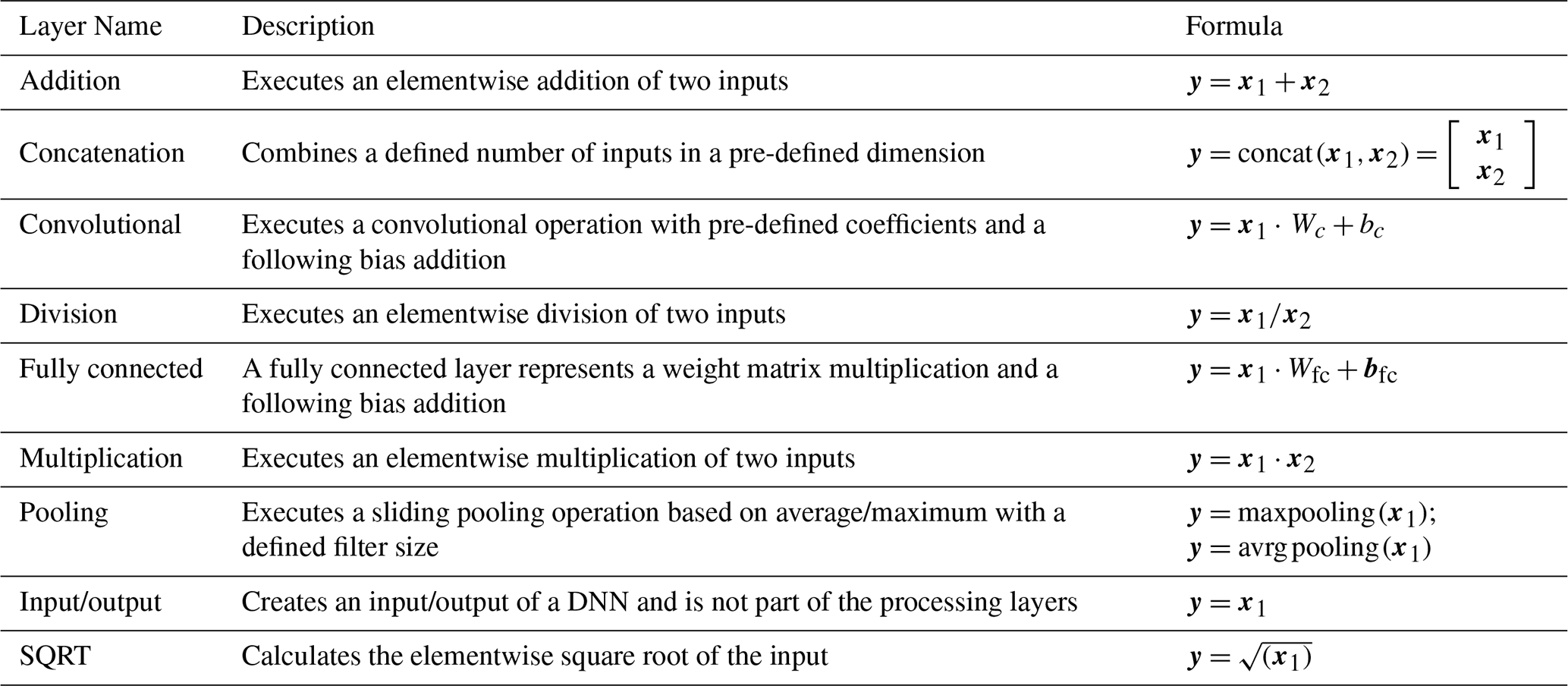
2.4 Neural network layers

The method for representing the inference of a trained explainable ML as a DNN is based on different Layers. The most important and used layers are briefly described in Table 2 and defined in the Open Neural Network Exchange (ONNX, 2023) operation set.

Table 2 List of used neural network layers.

2.5 Datasets

The datasets used in this study are open source and are from the fields of PM, CM, gas sensing (GS), and structural health monitoring (SHM), which were investigated in other studies, which also include a comparison between the interpretable ML algorithms and CNN (Goodarzi et al., 2025). The following section briefly describes the datasets with their most important characteristics listed in Table 3.

Table 3 Overview of the datasets included in the benchmarks.

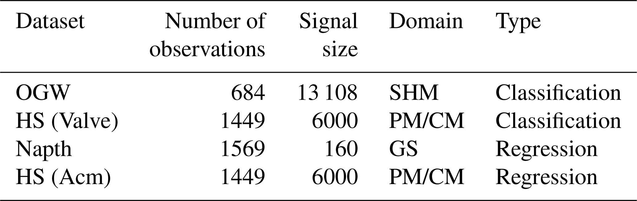
The open guided wave (OGW) dataset described in Moll et al. (2019) consists of time series signals that capture guided waves recorded at various temperature levels, ranging from 20 to 60 °C. The signals were collected using 12 ultrasonic transducers arranged in a sender–receiver configuration, where one combination was used for training. These transducers were attached to a carbon fiber reinforced polymer (CFRP) plate with a detachable aluminum mass positioned at four locations to simulate delamination damage. The goal is to detect whether there is damage or not.

The hydraulic system (HS) dataset is recorded at a hydraulic system testbed monitored with several sensors (Schneider et al., 2018a). The goal is to detect various fault conditions. The system variables valve state and hydraulic system accumulator are selected as the target variables for training the algorithm and, in this paper, are treated as two independent datasets: HS (Acm) and HS (Valve). The sensor that shows the best correlation with these targets is the pressure sensor in the work cycle (PS1).

The naphthalene (Napth) dataset (Bastuck et al., 2015) consists of recordings from a gas sensor operating at different temperatures. The sensor signals were sampled at a rate of 4 Hz. The dataset focuses on the quantification of the naphthalene concentration in the presence of ethanol as a background or interfering gas.

3 Deep neural network representation

The core of this paper is the novel approach to represent trained interpretable ML algorithms as DNN to accelerate them for an efficient implementation on edge hardware and intelligent sensors, e.g., to allow to the use of generic AI accelerator hardware. Section 3 breaks down the algorithms listed in Table 1 into the basic mathematical operations and gives a detailed description of the corresponding DNN representation. The DNN representations of the following algorithms serve as examples of a method that can also be applied to other ML algorithms. The section first describes the equation or the structure of each FE algorithm inference and then shows a detailed layer graph of the DNN representation. The parameters, which were determined in the previous training process, are represented through weights, bias, filter coefficients and other layer parameters to infer them on limited edge hardware.

3.1 Feature extraction

3.1.1 Adaptive linear approximation

The adaptive linear approximation (ALA) extracts information in local details, like edges in the time domain. ALA divides the input data y_i into k non-equidistant signal segments, based on the number of samples t_i, and for each segment extracts their mean ${\stackrel{\mathrm{‾}}{y}}_k$ and slope b_k. The non-equidistant splitting does not allow the average pooling layer to be used to calculate the mean. Instead, the mean must be calculated within a fully connected layer, represented in Fig. 4, based on the starting indices for each segment v_k.

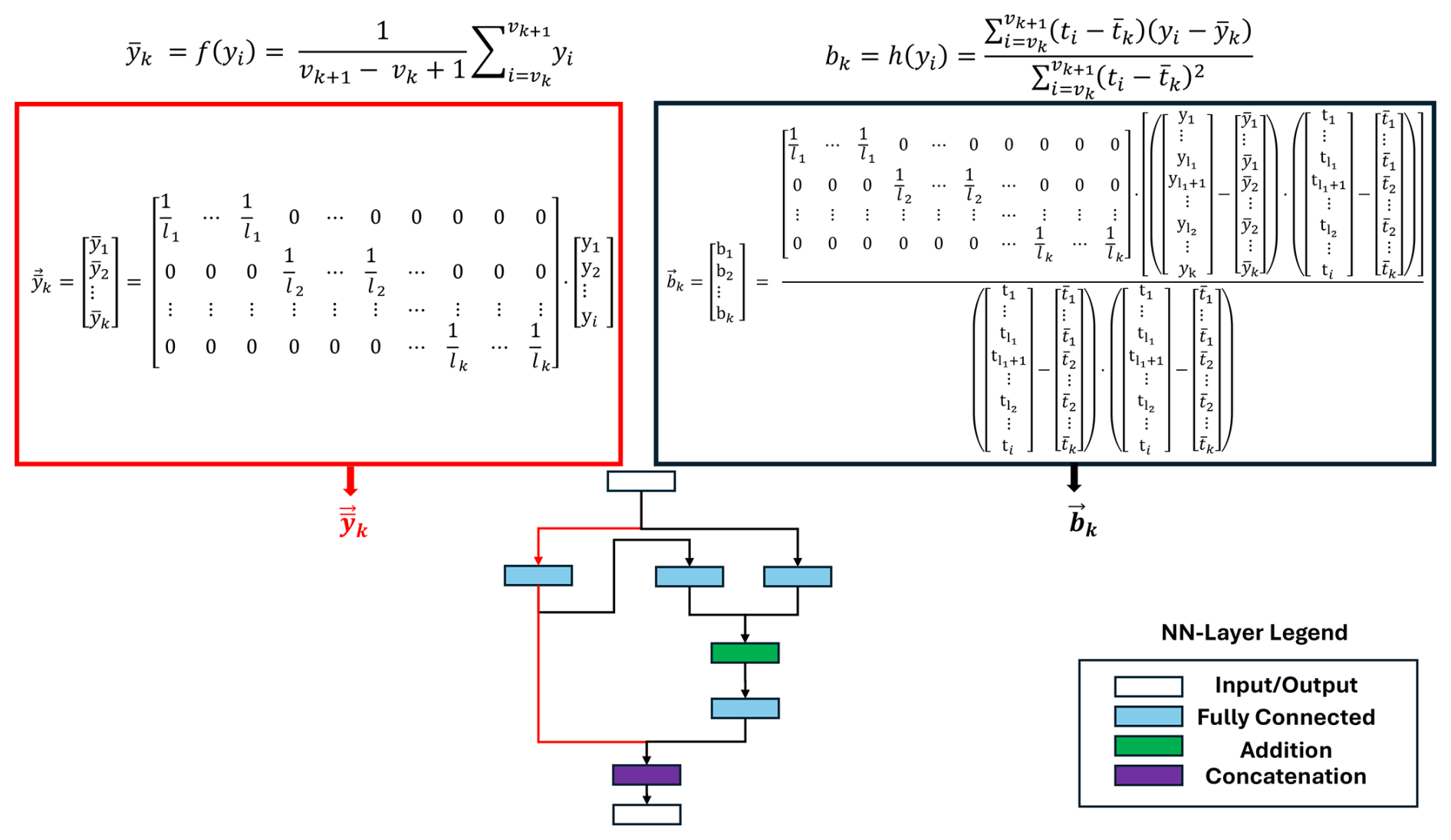
Figure 2 Representation of the adaptive linear approximation extractor as a deep neural network.

The parameters l_k describe the length of each segment and are calculated as $l_k=v_{k+\mathrm{1}}-v_k$. The slope calculation consists of four fully connected layers and one addition layer, representing the formula for b_k in Fig. 2. The term in the nominator is constant for each segment, determined in the previous training process, and can be calculated within a fully connected layer without using an additional division layer.

3.1.2 Best Daubechies wavelets

The wavelet transformation is able to transform the input signal into a time–frequency representation to extract locally high-frequency and temporally localized features of the signal. The benefit of the wavelet transformation is that it offers low resolution in the time domain and high resolution in the frequency domain for high-frequency signals and vice versa for low-frequency signals. The discrete Wavelet transform is based on discretely sampled wavelets. A very efficient way to implement the discrete Wavelet transform is to implement it as a filter bank. The filter bank represents a low-pass and high-pass filter sequence (see Fig. 3) with filter coefficients g and h.

Figure 3 Representation of the best Daubechies wavelet extractor as a deep neural network.

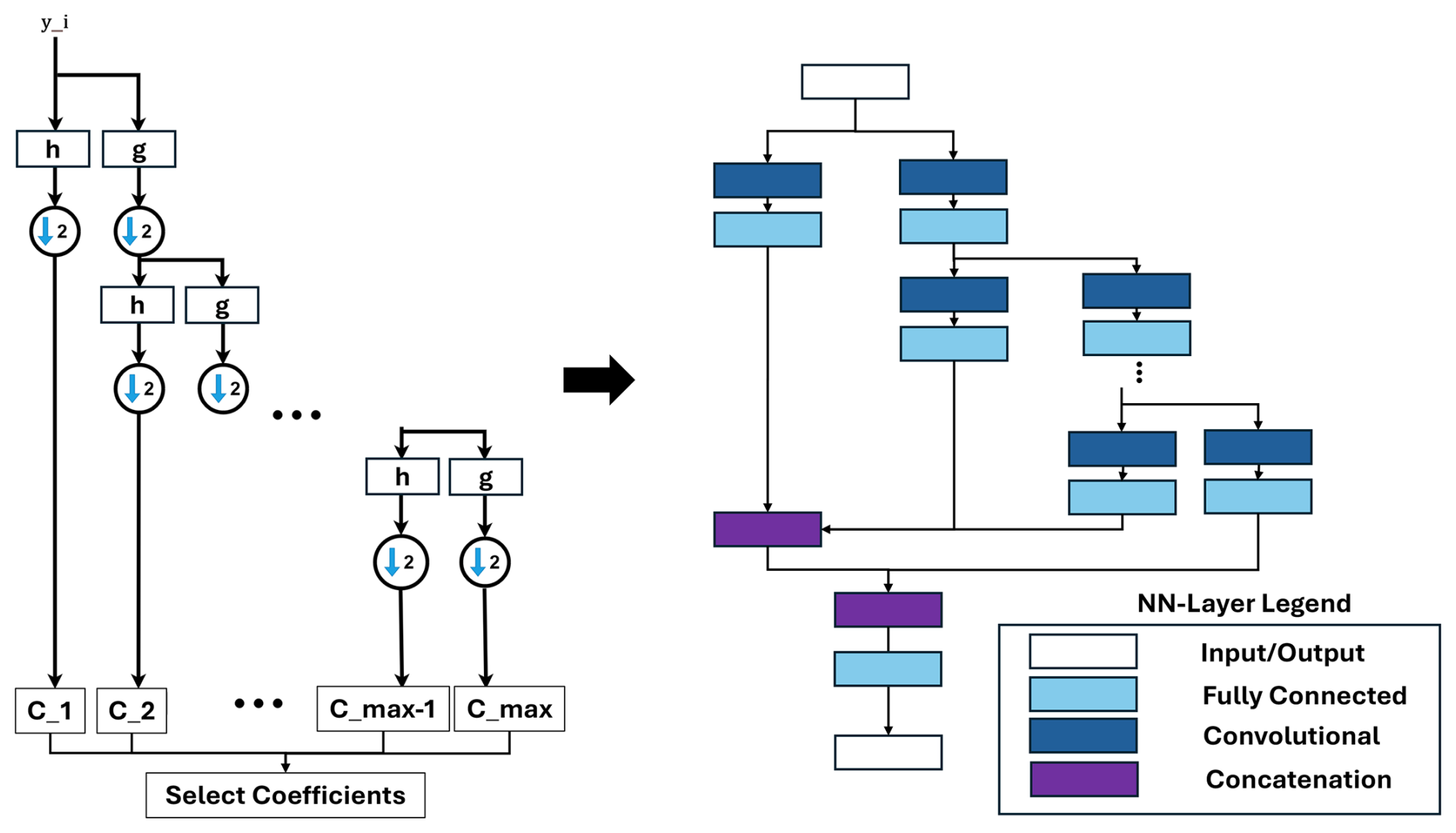
The DNN representation rebuilds the wavelet transformation's filter stages, including the coefficient multiplication and the downsampling process. Before the DNN is created, the filter coefficients and the number of filter stages are calculated based on the available data. The different filters are represented by convolutional layers with wavelet function-specific coefficients. The algorithms calculate, in addition to the transformation, ranking of the coefficients based on the absolute value. After the ranking only the best coefficients with the highest absolute value are considered in further calculation. This selection is performed with an additional fully connected layer.

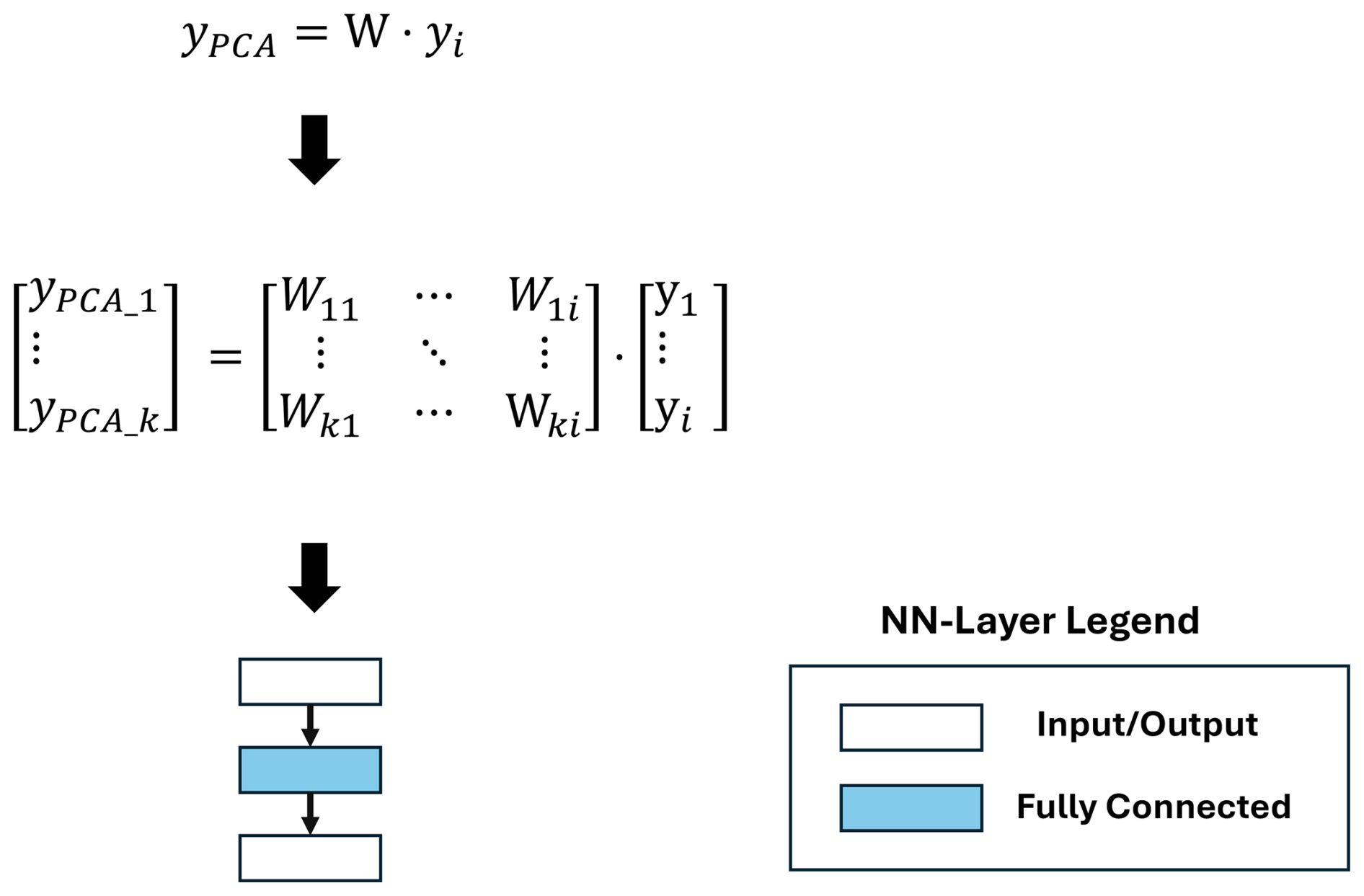
3.1.3 Principal component analysis

The principal component analysis (PCA) transforms the input data to extract information and features in the general cycle shape. The PCA reduces the input dataset's dimensionality by applying an orthonormal coordinate system transformation keeping only the first dimensions representing the highest variance or information content. The first PC is the axis in the new calculated coordinate system, which explains the most variance in the dataset. The second one explains the second largest variance, and with decreasing PC, the explained variance decreases. This allows for the reduction of the dimensionality with a minimal loss of information. After training, the inference of the PCA transformation y_PCA can be calculated within a fully connected layer with zero bias, and the weight matrix W presents the PCA transformation coefficients as pre-defined weights. So the PCA transformation only consists of one fully connected layer in the DNN representation as shown in Fig. 4.

Figure 4 Representation of principal component analysis as a deep neural network.

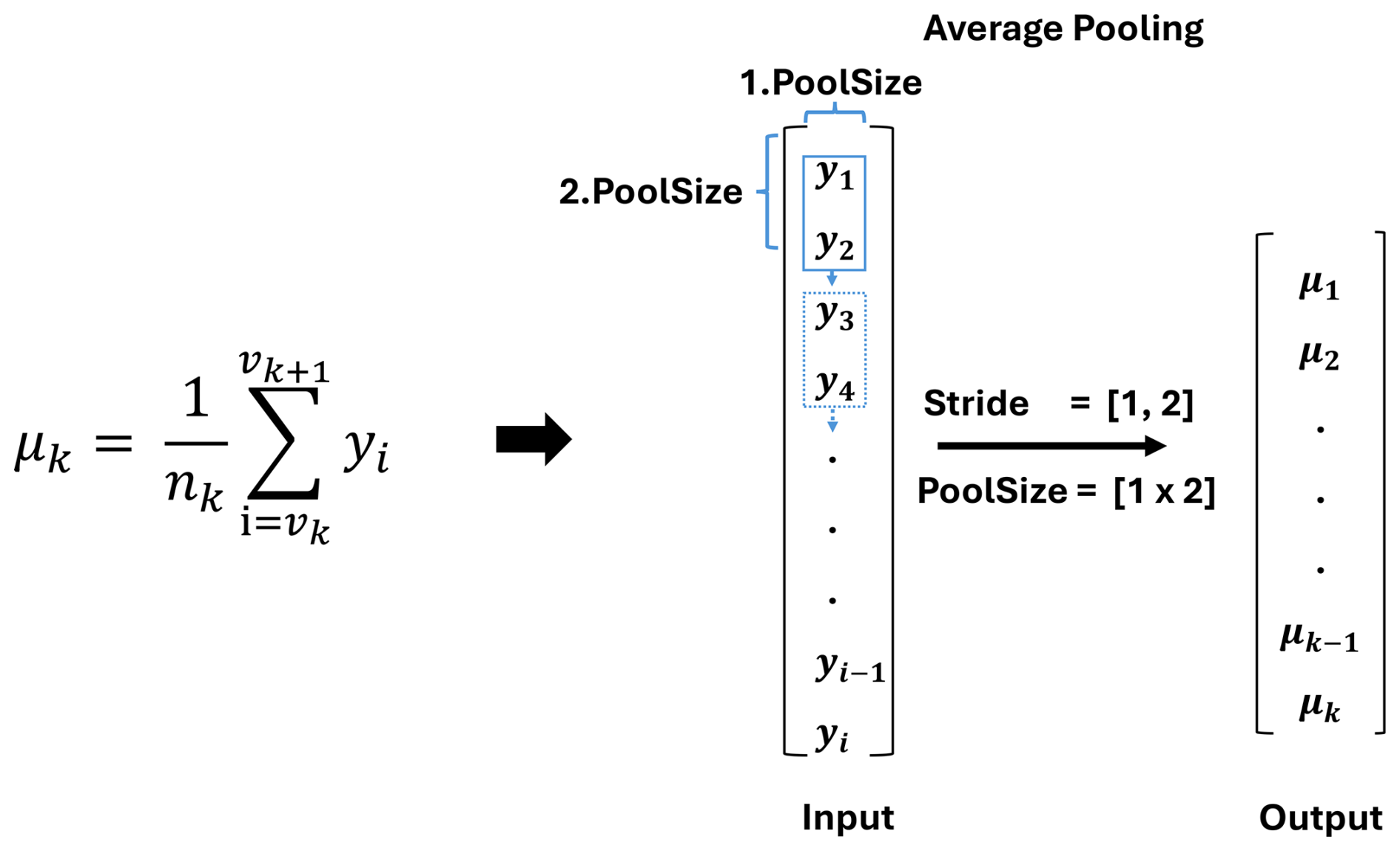
3.1.4 Statistical moments

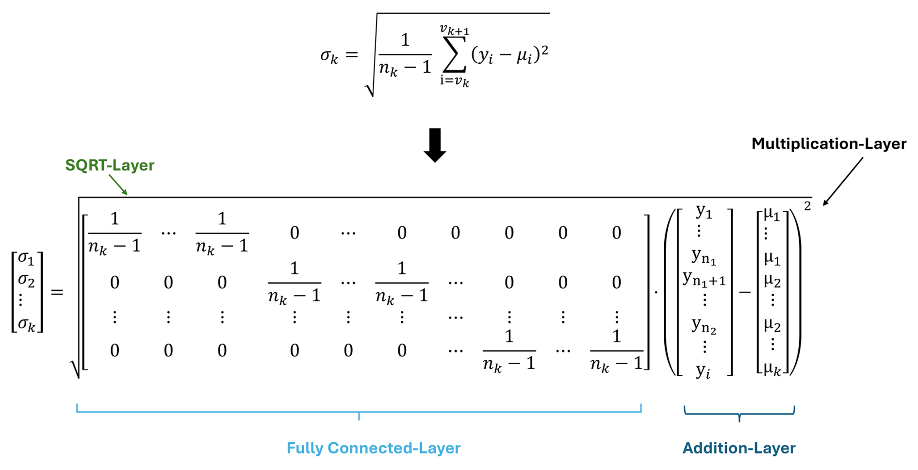
The statistical moment algorithm can describe the empirical distribution of single measurement samples. This FE method calculates the first four empirical statistical moments of the signal sample, providing information about its characteristics in the time domain. The first four statistical moments are the mean μ_k, the standard deviation σ_k, the skewness v_k, and the kurtosis w_k. One time signal is divided into segments of equal length to gain a more specific description of the raw data. This segmentation allows an arbitrarily precise description of the statistical distribution of the signal. Since the method divides the data into equidistant segments, the calculation of the mean can be represented by an average pooling within the DNN (see Fig. 5). The filter size of the pooling layer should have the same size as the equidistant signal segments of the input signal. In the example, the segment size equals two and is initialized through the filter size in the pooling layer. The mean of the signal is then calculated as follows and is represented by an average pooling layer, where v_k describes the start indices of the corresponding segment. The end indices of each segment are then described with v_k+1.

Figure 5 Representation of mean calculation with an average pooling layer.

The standard deviation in Fig. 6 within the DNN is based on the previous calculation of the mean of each signal segment. The previous calculated mean is resized within a fully connected layer. The layer creates a new vector μ_i with the size of the input data i. The vector consists of a concatenation of each mean value μ_k for the corresponding length of the segment n_k. This allows a simple subtraction of the mean value of each segment. This subtraction is executed by multiplying with “−1” using a convolutional layer followed by an addition layer. The sum and the division by (n_k−1) are performed within a fully connected layer, as shown in Fig. 6. The parameter n_k represents the length of each segment. The last step is calculating the square root within a SQRT layer.

Figure 6 Representation of variance calculation with different deep neural network layers.

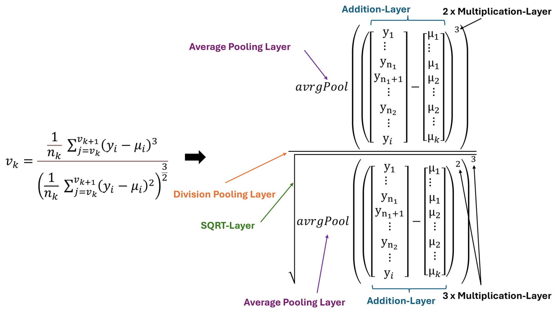
To calculate the skewness, i.e., the third statistical moment, the sum of the standard deviation is reused. The difference is the factor of the division, which changes to $\frac{\mathrm{1}}{n_k}$ but is also divided within a fully connected layer with a sparse matrix. The denominator is calculated by the three-time self-multiplication of the standard deviation based on two element-wise multiplication layers. The numerator is the three-time self-multiplication of the difference between the signal and the mean. An elementwise division layer executes the final calculation (see Fig. 7).

Figure 7 Representation of skewness calculation with different deep neural network layers.

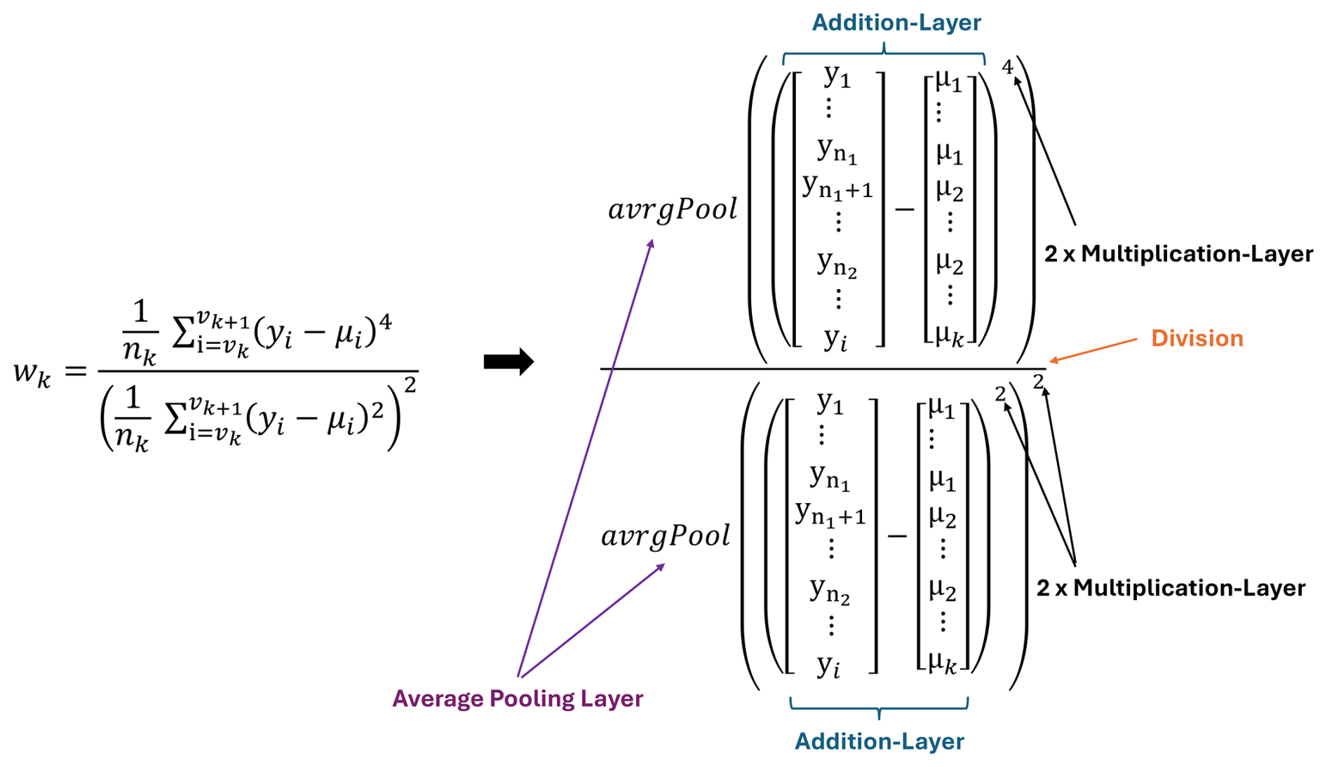
The calculation of kurtosis, i.e., the fourth statistical moment, is the same as the calculation of skewness, with the difference of the potency value of the numerator and denominator (see Fig. 8).

Figure 8 Representation of kurtosis calculation using deep neural network layers.

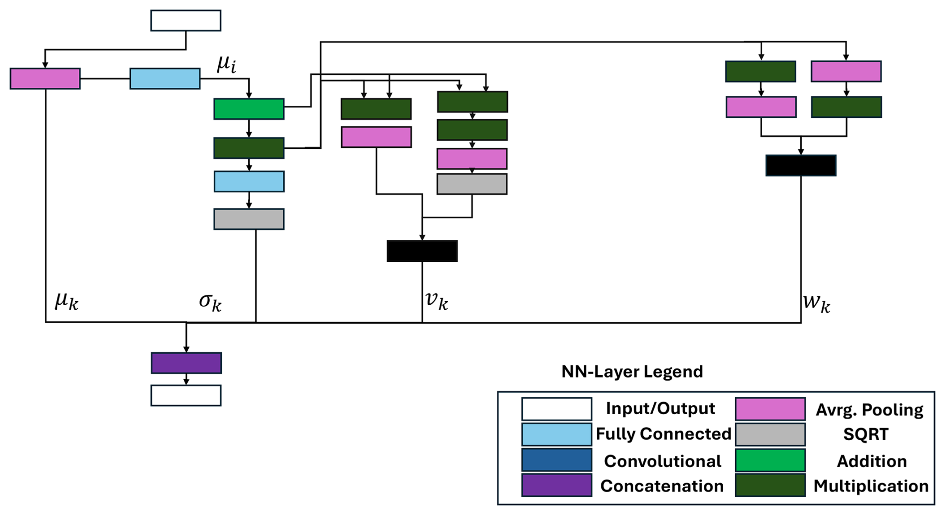
The combination of the calculation of all different features is shown in Fig. 9. Each feature can be seen as a separate calculation path in the DNN, and the paths are combined with a concatenation layer. The features that build the basis for further features are reused within the network and can be seen as connections between different paths. Additionally, most of the fully connected layers have weight matrices, where most entries are zeros, which increases the sparsity value of the DNN.

Figure 9 Representation of the statistical moment extractor as a deep neural network.

3.2 Feature selection

A feature selection algorithm is trained for further dimensionality reduction. The selection algorithm keeps a subset of the previously calculated features. It removes redundant, noisy, and irrelevant features to improve the algorithm's accuracy and avoid overfitting. The FS algorithms are implemented because of the fully automated conversion from the ML Toolbox but would normally not be necessary for the inference on which the paper is focused. However, when extending supervised methods with semi-supervised methods for novelty detection, which require all features (Klein et al., 2024), then a simple filter is needed to retain only the selected features for the inference. Table 4 briefly describes four FS algorithms included in the ML Toolbox.

Table 4 Feature selection algorithms.

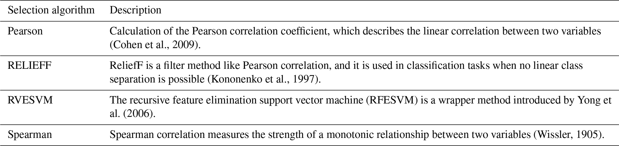
The output of each trained algorithm is a vector ranking the features based on their information value. As shown in Fig. 10, just one fully connected layer can be used to map the FS algorithm to DNN.

Figure 10 Representation of the feature selection algorithms as a deep neural network.

3.3 Classification and regression

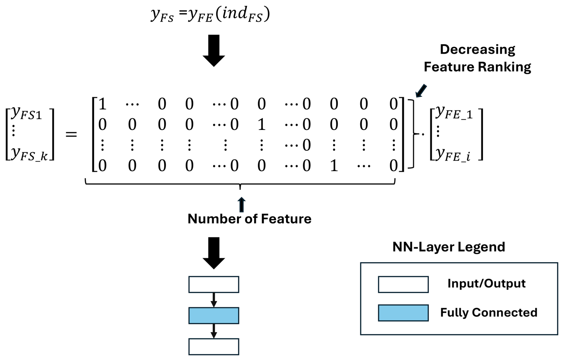
3.3.1 Partial least squares regression

Partial least squares regression (PLSR) is a supervised ML algorithm designed to model the correlation between the target variable and the features calculated by subsequent FE and FS steps. PLSR is particularly useful for overcoming collinearity in linear regression and handling cases with sparse observations. During training, the PLSR learns the best linear transformation based on the calculated vector w. The vector is multiplied with the extracted features and results in the prediction $\widehat{y}$. This prediction of the regression algorithm can be represented by a single fully connected layer (see Fig. 11).

Figure 11 Representation of partial least squares regression as a deep neural network.

3.3.2 Linear discriminant analysis and Mahalanobis distance classification

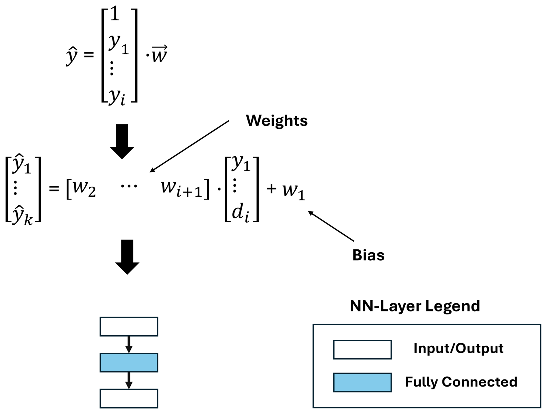
The linear projection executed by linear discriminant analysis (LDA) first transforms the feature space into a new, (k−1)-dimensional space by maximizing the between-class scatter and minimizing the within-class scatter. The dimension k describes the number of classes within the used dataset and i the length of the input signal. After the linear transformation is learned on the used dataset, the execution to calculate the LDA transformed Y_LDA can be represented by matrix multiplication of the transformation matrix W and the extracted features of a sample y_FS. The matrix is calculated with supervised learning and can be replaced with a single fully connected layer in DNN representation with zero bias, comparable with the PCA transformation (Fig. 12).

Figure 12 Representation of linear discriminant analysis as a deep neural network.

After the linear transformation, the Mahalanobis distance to each class is calculated. The Mahalanobis distance is based on the covariance matrix S_{class_k}, where k denotes the class number, the LDA transformed data Y_LDA, and the arithmetic mean x_k. Based on the formula in Fig. 13, the calculation of the Mahalanobis distance to one class can be executed by three fully connected, two addition, and one multiplication layer.

Figure 13 Representation of the Mahalanobis distance of each class as a deep neural network.

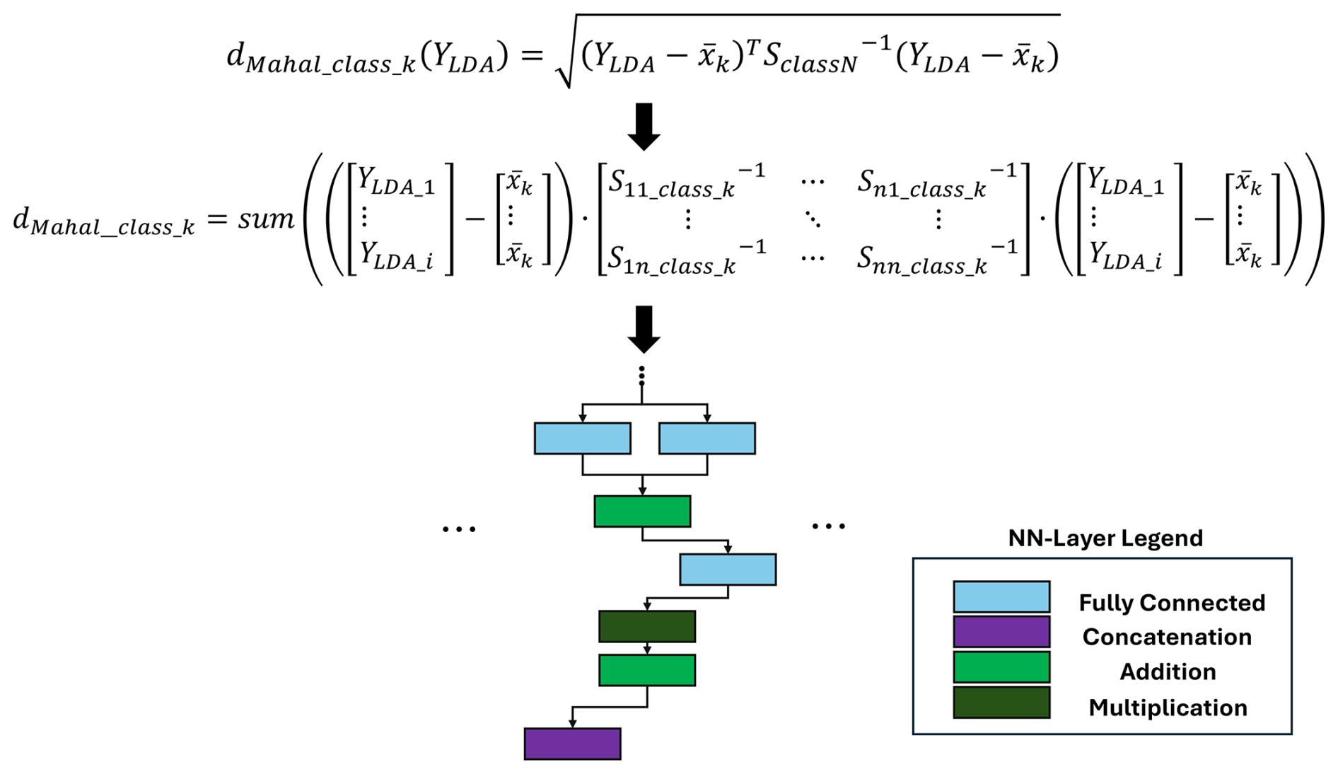
As shown in Fig. 14, each distance to the different classes must be calculated. The complete DNN size depends on the number of classes available in the dataset, as demonstrated in Fig. 14. The actual classification is based on the calculated Mahalanobis distance to each class. To extract the lowest distance, the calculated Mahalanobis distances are concatenated and multiplied by minus 1, within a convolutional layer. The index of the largest value in the resulting vector is calculated with a max pooling layer and equals the class number with the lowest Mahalanobis distance (see Fig. 14).

4 Results

The results presented are based on the automated methods provided by the ML Toolbox (ZeMA-gGmbh, 2017). As mentioned earlier, the toolbox provides an automated algorithm search for the desired input data and corresponding targets. As a result, the best combination of FE, FS, and C/R algorithms is identified based on the best accuracy achieved with 10-fold cross-validation. The optimal combination of methods is trained and subsequently converted to a DNN representation for each dataset individually, as described in Sect. 3. Figure 14 illustrates a converted model consisting of the StatMom extractor, Pearson selection, and LDA-MD distance classifier trained, on the HS (Valve) dataset as a classification problem. The combination of individual algorithms results in a sequential chaining of each algorithm to the other. As shown in Fig. 14, each signal processing step remains interpretable and can be visualized after the layers corresponding to that specific step. A corresponding implementation is performed for the other three datasets.

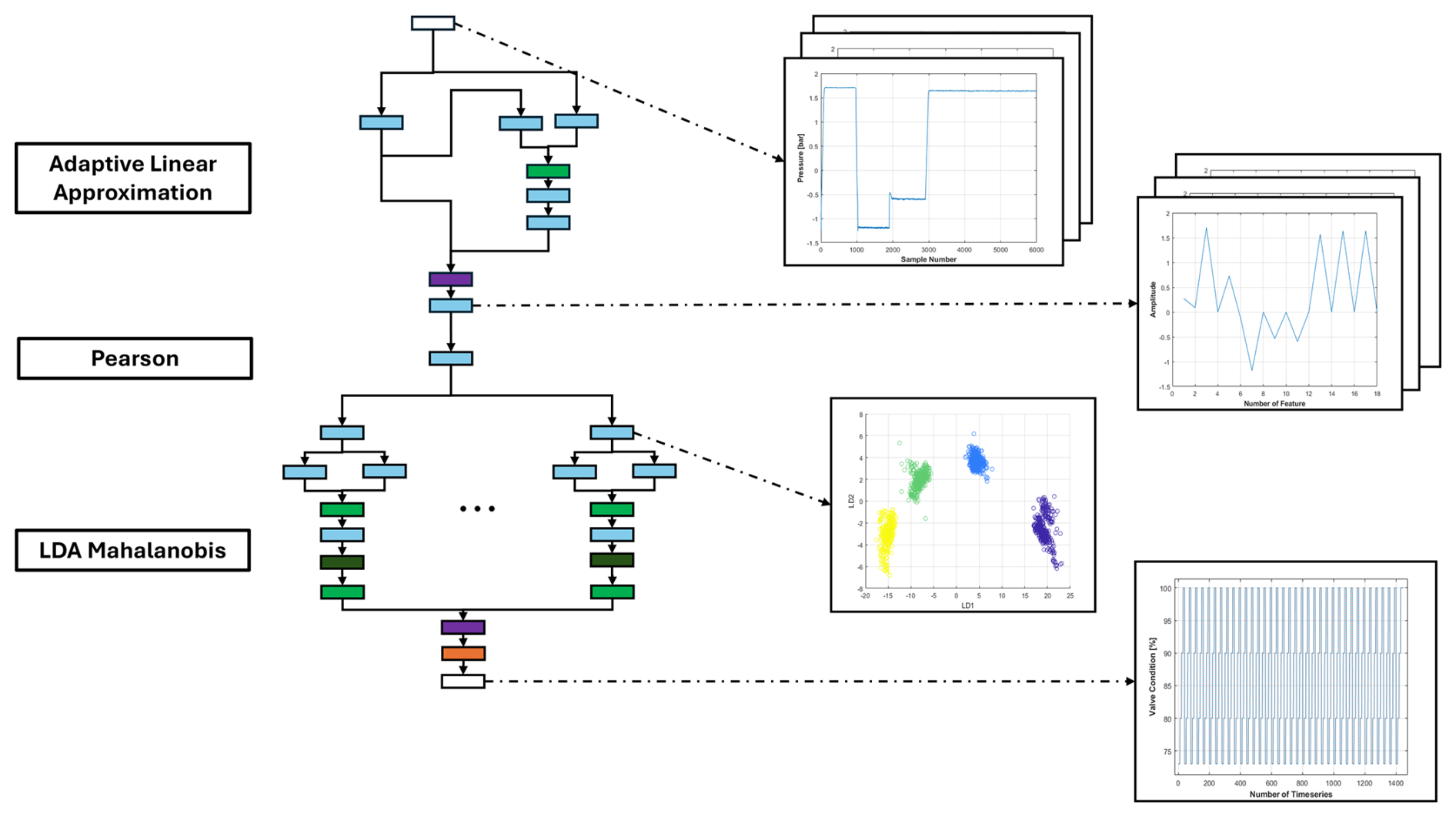
Figure 14 A complete FESC/R algorithm, consisting of ALA extraction, Pearson correlation selection, and LDA-MD classifier as a deep neural network trained on the HS (Valve) dataset.

4.1 Metrics

4.1.1 Accuracy

The study of the accuracy of the DNN representation involved four different datasets, described in Sect. 2. The evaluation consists of two regression and two classification problems. The datasets were selected to use every implemented FE, FS, and classification/regression algorithm. The best FESC/R algorithms and the results for three different DNN representations are listed in Table 5. The table details the optimal algorithm combinations from the toolbox, along with the classification and regression errors for the FP32, INT16, and INT8 versions of the algorithms and DNN representations. The accuracy of the FP32 version of the DNN representation matches exactly with the original MATLAB algorithm, indicating correct implementation of the ML stacks as DNN.

Table 5 Accuracy of the different deep neural network representations for each dataset.

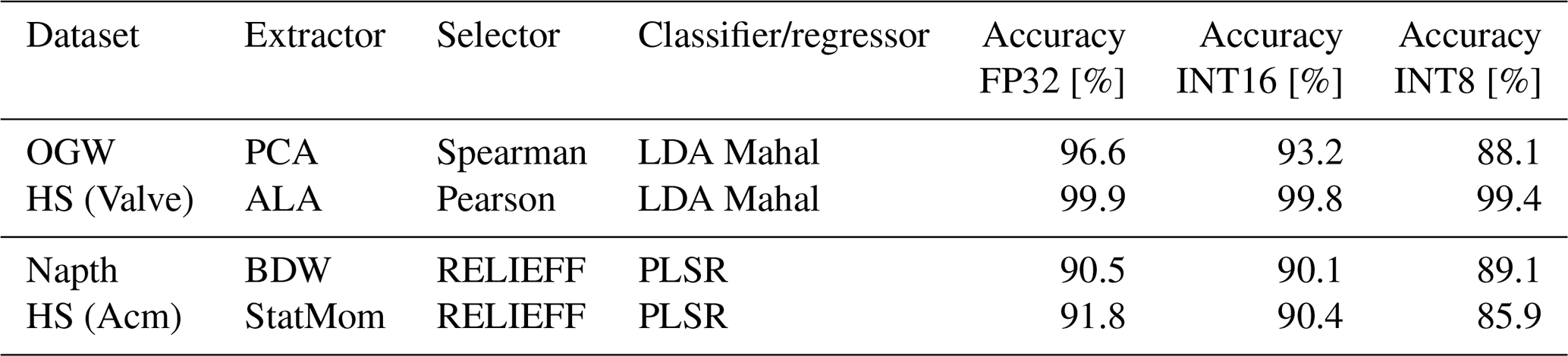
For all four datasets, the 10-fold cross-validation classification accuracy is nearly perfect, with the lowest accuracy being 96.6 % for the OGW dataset for the classification and 90.5 % for the Napth as a regression problem. With decreasing data precision, the accuracy of each model also decreases. Quantizing the DNN into an INT16 model results in a maximum accuracy drop of 3.4 % for the OGW dataset and 1.4 % for the HS (Acm) dataset. In the further step, the quantizing to the lowest precision, INT8, results in a significant accuracy drop compared to the FP32 version. The largest drop was observed on the OGW dataset with 8.4 % for the classification and 5.9 % in the HS (Acm) for regression. To summarize, the accuracy of a DNN representation decreases as precision is reduced, as shown in Fig. 15.

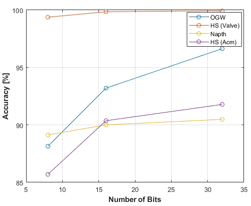
Figure 15 The accuracy of the four different datasets as a function of the number of bits used including 32-bit, 16-bit, and 8-bit usage.

4.1.2 Memory requirements

The memory used can estimate the hardware's requirements in terms of storage size. The size of the ONNX network is measured and shown in Fig. 16. Fortunately, specialized hardware also allows the efficient storage of sparse matrices. Figure 16 shows the sparsity of all DNN representations studied in this paper. The DNN representations show a significant sparsity value of at least 90.2 % (see Table 6). So the real memory requirement can be calculated by multiplying the measured requirement with the sparsity and subtracting this number from the measured memory requirement. Especially the regression datasets resulting in DNN with small memory requirements up to 19 kB for the HS (Acm) data. Compared to the classification datasets, the memory requirement reaches up to 970 kB, the regression task represents the lower memory requirement.

Table 6 Accuracy of the different deep neural network representations for each dataset.

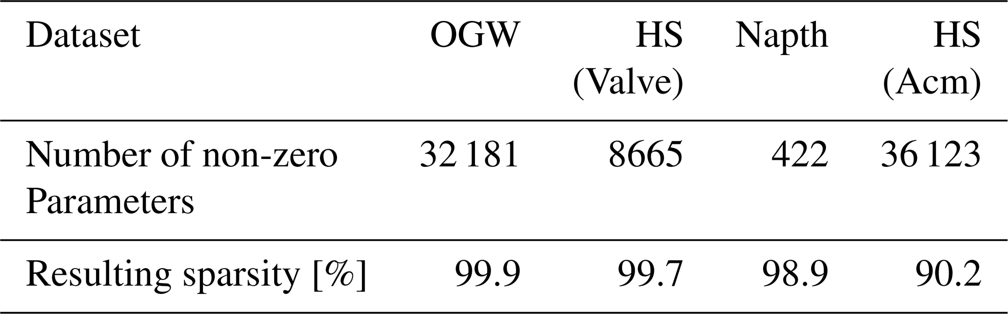
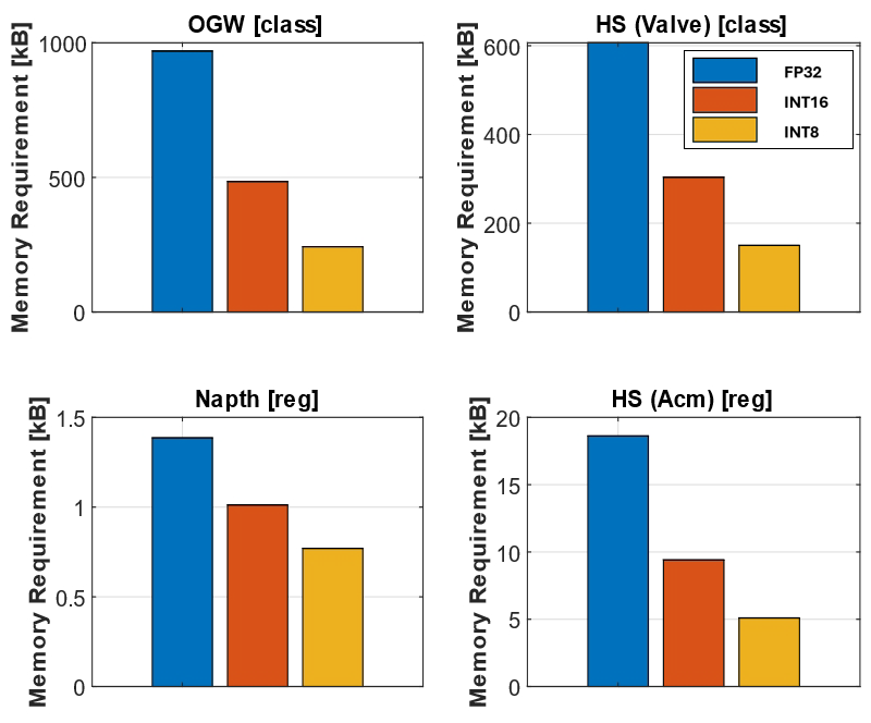
Figure 16 Memory requirements of the deep neural network representations including the sparsity of the deep neural networks.

In conclusion, the memory requirement is strongly correlated with the input data length and the task type executed. The classification algorithms result in higher memory usage than the regression algorithms. The comparison of the OGW algorithm and the HS (Valve) algorithm demonstrates the strong influence of the input data length regarding the required memory. As expected, the quantization reduced the size from FP32 to INT8 to nearly a quarter of the size for each algorithm.

4.1.3 Runtime

The runtime comparison ran on the Karo board (Karo electronics, 2025). The comparison includes the run as a Python implementation on the CPU and the DNN representation within a Python script on the CPU. The comparison excludes the INT16 representation of the FESC/R algorithms as this cannot be run efficiently on the edge hardware. In the current version, the ONNX runtime (ORT) package does not support the efficient inference of the INT16 version. The time given represents the model prediction for 10 000 serial input data, simulating the serial recording of a sensor. The ORT library is used to infer the DNN representation. The means of the other results are listed in Table 7.

Table 7 Mean runtime comparison of the different deep neural network representations for each dataset for 10 000 predictions.

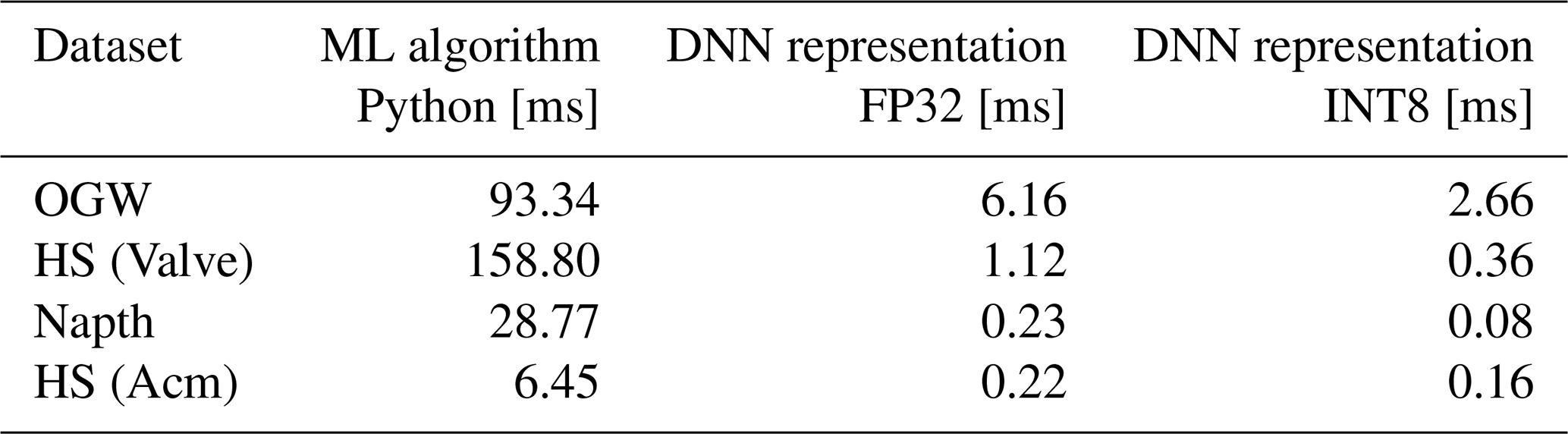
The DNN representation results in large improvement compared to the typical Python libraries implementation regarding the runtime. The runtime of the DNN in FP32 for the HS (Valve) was reduced by 99.3 % compared to the common Python implementation and demonstrates the largest improvement. The other runtimes were reduced by 96.6 % for the HS (Acm), 99.2 % for the Napth, and 93.3 % for the OGW dataset, comparing FP32 DNN with the common Python implementation. The further quantization of the DNN to the INT8 version leads to a further runtime reduction of 56.9 % for the OGW, 67.7 % for the HS (Valve), 64.8 % for the Napth, and just 25.4 % for the HS (Acm) comparing INT8 inference to the FP32 DNN inference.

5 Discussion

This paper presents an efficient method to represent pre-trained and interpretable ML algorithms as DNNs to implement them efficiently on edge hardware. The approach was based on breaking down the static inference equation into basic mathematical operations to replace them with generic DNN layer functions. Besides the efficient implementation, this enables different hardware implementation optimization techniques like quantization. The new approach and associated techniques were studied in this context with respect to the accuracy and memory requirements for the different DNN versions. Furthermore, the runtime performance was compared to a standard Python implementation for each model inference. The benchmarks are based on four datasets from different application fields (gas measurement, predictive maintenance/condition monitoring, and structural health monitoring).

The results of the benchmarks demonstrated efficiency in terms of runtime and memory requirement, as well as the quantization technique introduced from the DNN optimization. Besides the gained optimizations, the method allows a rough estimation of the hardware requirements of the implemented DNN representation. The presented method allows one to find a good balance between memory requirements and runtime regarding the loss of accuracy. This paper demonstrates the potential of achieving a greatly reduced runtime and memory requirement on limited edge hardware, even before the use of optimized AI accelerators. Regarding runtime, the DNN representations reduced the runtime by up to 99.3 % compared to common implementations and a further reduction of 67.7 % regarding the INT8 version. Additionally, the memory requirements were reduced by up to 73.4 % by converting the FP32 model into INT8 models, with a drop in accuracy, which has to be considered. The DNN representation consists of sparse weight matrixes, which allows for a further decrease in implementation memory requirements. Furthermore, the chosen data type hardly influences the interpretable ML algorithms. A decrease in the data precision often results in a significant drop in the model's accuracy. This is partly caused by the different scale of the extracted features, which are calculated in the same layer, i.e., within a fully connected layer. PTQ defines a single scaling factor for the entire layer. Due to the wide range of feature values, this can result in significant information loss.

6 Conclusion and future work

In conclusion, trained explainable ML algorithms can be represented by DNNs to implement them on limited hardware. This paper showed that several mathematical and statistically based ML algorithm inferences can be represented by DNN layer functions, which also allows the usage of common DNN-optimized AI accelerators. This paper also visualized the potential of interpretability within the different DNN stages and the wide range of application fields of interpretable ML algorithms based on the FESC/R structure. The approach presented in this paper outperformed state-of-the-art Python implementations for inference on limited hardware. It also demonstrated the successful usage of common DNN techniques, like quantization, to further improve the runtime and memory requirements of the interpretable ML algorithm. For further improvement of memory requirement and runtime performance, the step of FS should be excluded from the inference process. Instead of selecting some of the previous extracted features, the focus in inference should be to only calculate the important features of the raw data, which are necessary for the performance of the algorithm. This future implementation step will further decrease the number of parameters of the DNN and also increase the runtime performance. Note that this can only be applied if a pure supervised ML model is required. If in addition also semi-supervised models are desired, i.e., for novelty detection or for recognizing out-of-distribution (OOD) data, then all features should be calculated (Klein et al., 2024). In further investigation, different standardization or normalization techniques should be introduced to decrease the accuracy drop caused by the quantization. The runtime comparison displays an excellent first outlook of how efficiently interpretable ML can be implemented on edge hardware without further effort, but this study only considered the CPU usage of the dedicated hardware. A further investigation of different AI accelerators, which are now useable, without any further effort, for the interpretable ML algorithms, is crucial for demonstrating further improvements. The further comparison should also include the usage of generic AI accelerators like NPUs, TPUs, and GPUs. This efficient implementation should be compared to lower-level programming languages like C/C$++$ to highlight the improvement. An additional focus here should be on investigating energy efficiency and runtime improvements, which expands the investigations from a previous study (Schauer et al., 2024c). Furthermore, the investigation of common transfer learning (TF) techniques should be considered (Tan et al., 2018). Because of the limited selection of TF techniques, mainly consisting of standardization and normalization, to retrain interpretable ML algorithms, the now available options of common DNN TF techniques represent a further research topic.