Detection of geomagnetically induced currents on single phases in power grids using a fiber optic current sensor system

Power transformers are an integral part of our electric power system. Parasitic direct currents in the alternating-current grid cause inefficient transformer operation and demand mitigation measures to protect the grid’s constituents. In particular, geomagnetically induced currents (GICs) arising from solar activity prove to be an unpredictable risk for grid operators. Within this paper, we present an interferometric fiber-optic current sensor system designed for long-term monitoring of GICs, allowing fully remote sensor control and data access. The developed sensor possesses a noise-limited threshold sensitivity of 2.64 mA ${\sqrt{\mathrm{Hz}}}^{-\mathrm{1}}$. We successfully demonstrate the first optical measurement of GICs on a single phase of the power grid during two distinct geomagnetic events, on both the low-voltage and the high-voltage sides.

1 Introduction

Ensuring proper functionality and operation of the power grid is of utmost importance given the importance of electrical energy supply in our daily life. Low-frequency currents (LFCs) with a frequency lower than 1 Hz, also called quasi-direct currents (DCs), in the alternating-current (AC) grid affect the operation of power transformers. These parasitic DCs or LFCs produce a positive or negative offset in the alternating flux of the transformer core. The resulting additional flux can lead to partial core saturation, causing distorted voltage and current waveforms, higher acoustic noise, and higher reactive power consumption. Furthermore, when the transformer core is saturated, the amount of active power that can be transferred is reduced (Albertson et al., 1993; Bachinger et al., 2013). In extreme cases, the transformer might overheat, leading to its destruction (Gaunt and Coetzee, 2007).

The probability of DCs appearing in the interconnected European grid may increase due to the ongoing energy transition and the growing adoption of power electronic devices (Gertmar et al., 2012). DCs in the power grid can also arise from variations in the Earth's magnetic field, which are influenced by solar activity. Charged particles emitted during solar flares compress and stretch the geomagnetic field, inducing currents within the power grid. These currents are known as geomagnetically induced currents (GICs) and may reach magnitudes ranging from a few to hundreds of amperes, depending on the latitude (Pirjola, 1989). While there are small amounts of parasitic DCs present in the AC power grid at all times, originating from the aforementioned humanmade sources, GICs may be predicted from space weather satellite data and are preceded by sudden changes in the geomagnetic field.

Given their aperiodic occurrence and varying amplitude, it is of great interest to facilitate long-term monitoring of GICs in order to preserve the functionality of the grid. Existing measurement solutions have used a zero-flux current transducer (CT) system (Moore et al., 1988) in the transformer neutral point on ground potential (Albert et al., 2022). Due to the constraints of conventional CTs – such as the need for isolation, saturation, or electromagnetic interference effects – and incompatible sensor dimensions, a measurement on high-voltage (HV) potential has not been realized yet. Thus, there are still no real-world data about the distribution of GICs on the grid's three phases and their splitting on individual lines, which are predicted by existing simulations (Bailey et al., 2018), and such data would provide valuable information for the effective employment of mitigation measures.

Optical CTs, such as fiber-optic current sensors (FOCSs), are promising candidates for this task. Using optical fiber as the sensing medium, they provide inherent galvanic separation from the circuit and enable simultaneous measurements of ACs and DCs on HV potential. Furthermore, the favorable form factor of the FOCS sensing head allows retrofitting of existing structures in the power grid, while the devices for operating the sensor and data acquisition may be kept at a safe distance from the measurement site.

In this work, we present a fiber-optic current sensor system specifically designed for monitoring geomagnetically induced currents in the 50 Hz alternating-current power system. The sensor is equipped with an onboard electronics module that performs signal processing, stores data, and allows remote data access and sensor control. With this system, we show the first measurement of geomagnetically induced currents on single phases under high-voltage potential, as well as on the low-voltage side of the transformer, captured during different geomagnetic events. Furthermore, analysis of the AC harmonics present in the signal allows predictions of the transformer's saturation behavior.

2 Sensor setup

The developed sensor builds on the concept of a polarization-rotated reflection interferometer, which has been introduced by Frosio and Dändliker (1994) and Blake et al. (1996).

Light from a superluminescent diode (SLD), centered at 1550 nm with a bandwidth of 60 nm (Exalos EXS210156-01), excites the orthogonal polarization modes of a polarization-maintaining fiber (PMF) at a 45° splice point at equal amplitudes. A LiNbO₃ phase modulator (iXBlue MPX-LN-0.1), which is driven with a sinusoidal signal, introduces a non-reciprocal phase shift between the two modes, before they are separated way beyond their coherence length through propagation in a PMF lead. This minimizes cross-coupling effects that would deteriorate the sensor signal. At the entrance of the spun fiber sensing coil, a $\mathit{\lambda }/\mathrm{4}$ retarder was produced from PMF using a method described by Bohnert et al. (2002). It converts the two orthogonal linear polarization modes into left- and right-hand circular polarizations, which then acquire a non-reciprocal phase shift caused by the current's magnetic field by means of the Faraday effect. After reflection, the effect doubles on the return trip. The resulting relative phase shift ϕ between the two modes is described by

$$\begin{array}{}\text{(1)}& \mathit{\varphi }=\mathrm{4}VNI.\end{array}$$

The phase shift is dependent on the Verdet constant V of the material, which has a value of about 0.7 µrad A⁻¹ at 1550 nm (Rose et al., 1997), and the number of fiber windings N around the conductor carrying the current I.

Due to the interchange of polarization axes at the mirror and the polarization conversion, a reciprocal optical path and immunity to external perturbations experienced by both modes are ensured, while the non-reciprocal Faraday phase shift remains. The two polarization modes are overlapped at the 45° splice on the return trip; one axis is blocked by the PM circulator, and the optical signal reaches the electronics module, where it is processed further.

For an infield application, the sensor can be considered to consist of three separate blocks. The light source, all bulk optical elements (including the phase modulator), and the electronics module (closed box in Fig. 1) are placed inside an electric cabinet. The components inside the cabinet are shielded from external influences, and heating ensures an ambient temperature of at least 25 °C. The following PMF, which is connected to the cabinet, serves as a lead to the measurement site. The sensing head consists of the $\mathit{\lambda }/\mathrm{4}$ retarder, the spun fiber (Fibercore SHB1500), and the fiber mirror – a commercial retroreflector (Thorlabs P5-SMF28ER-P01-1) with a short single-mode fiber pigtail that is spliced to the spun sensing fiber. These components are wound on a custom additive manufactured spool fitted to the dimensions of the conductor of interest. The use of spun fiber is a prerequisite for reliable long-term applications, as circular polarized modes are maintained against external influences due to the fiber's helical structure (Laming and Payne, 1989).

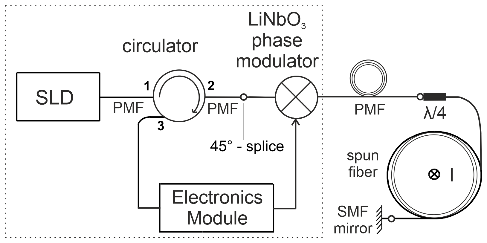
Figure 1 Principal scheme of the FOCS system: SLD – superluminescent diode, PMF – polarization-maintaining fiber leads, $\mathit{\lambda }/\mathrm{4}$ – fiber quarter wave retarder, I – current-carrying conductor, SMF mirror – single-mode fiber mirror. All elements in the enclosed box are placed in a cabinet far from the measurement site.

3 Signal processing

3.1 Electronics module

The developed electronics module takes over each task in the signal processing chain, from detection and data acquisition to data storage. The returning optical signal from the FOCS is converted into an electric signal by a photo diode (Thorlabs FGA01FC) and sent through an amplifier stage. A custom-made electronics board including a field-programmable gate array (FPGA) carries out the analog-to-digital conversion. Via an onboard digital-to-analog converter, the FPGA chip produces a sinusoidal drive voltage with adjustable frequency to control the LiNbO₃ phase modulator. The current-related phase shift can then be inferred from a Fourier analysis of the detected optical signal.

$$\begin{array}{}\text{(2)}& \mathit{\varphi }=\arctan \left[{\displaystyle \frac{J_{\mathrm{2}}\left(\mathrm{\Delta }{\mathit{\varphi }}_{\mathrm{0}}\right)}{J_{\mathrm{1}}\left(\mathrm{\Delta }{\mathit{\varphi }}_{\mathrm{0}}\right)}}{\displaystyle \frac{U\left({\mathit{\omega }}_{\mathrm{m}}\right)}{U(\mathrm{2}{\mathit{\omega }}_{\mathrm{m}}}}\right]\end{array}$$

The phase shift ϕ is retrieved from the relation of the voltage amplitudes U in the spectrum at the angular modulation frequency ω_m and the next harmonic 2ω_m. J_n is the Bessel function of the first kind at the value of the modulation depth Δϕ₀, which is given by Frosio and Dändliker (1994) as

$$\begin{array}{}\text{(3)}& \mathrm{\Delta }{\mathit{\varphi }}_{\mathrm{0}}={\mathit{\varphi }}_{\mathrm{0}}\sin \left({\displaystyle \frac{{\mathit{\omega }}_{\mathrm{m}}T}{\mathrm{2}}}\right),\end{array}$$

with ϕ₀ being the amplitude of the modulation signal and T the propagation time of light for one round trip between the LiNbO₃ phase modulator to the mirror. To obtain maximum sensitivity for the demodulation processing, ϕ₀ and ω_m may be selected so that J₁ is at its first maximum (Δϕ₀=1.84). Furthermore, modulating at the so-called proper frequency – when one full period of the sinusoidal modulation signal is equivalent to the time of flight T for the light in the interferometer – eliminates bias offsets in the even harmonics, which could lead to drifts over time, especially under changing ambient conditions (Lefevre, 2022). In the literature, there are also other approaches to signal recovery, such as choosing different values of the modulation depth for demodulation so that J₁=J₂ or including higher harmonics of the modulation frequency (Temkina et al., 2020).

From the calculated phase shift, the corresponding current is inferred from Eq. (1). The result is sent from the FPGA board via Ethernet to a commercial data hub (Artemes GmbH, Austria), which saves the data on a local hard disk drive and allows remote access via a modem using OpenVPN. Furthermore, this connection allows the remote setting of modulation parameters via the FPGA and a power reset of the electronics module. A schematic of the signal processing chain taken over by the electronics module is shown in Fig. 2.

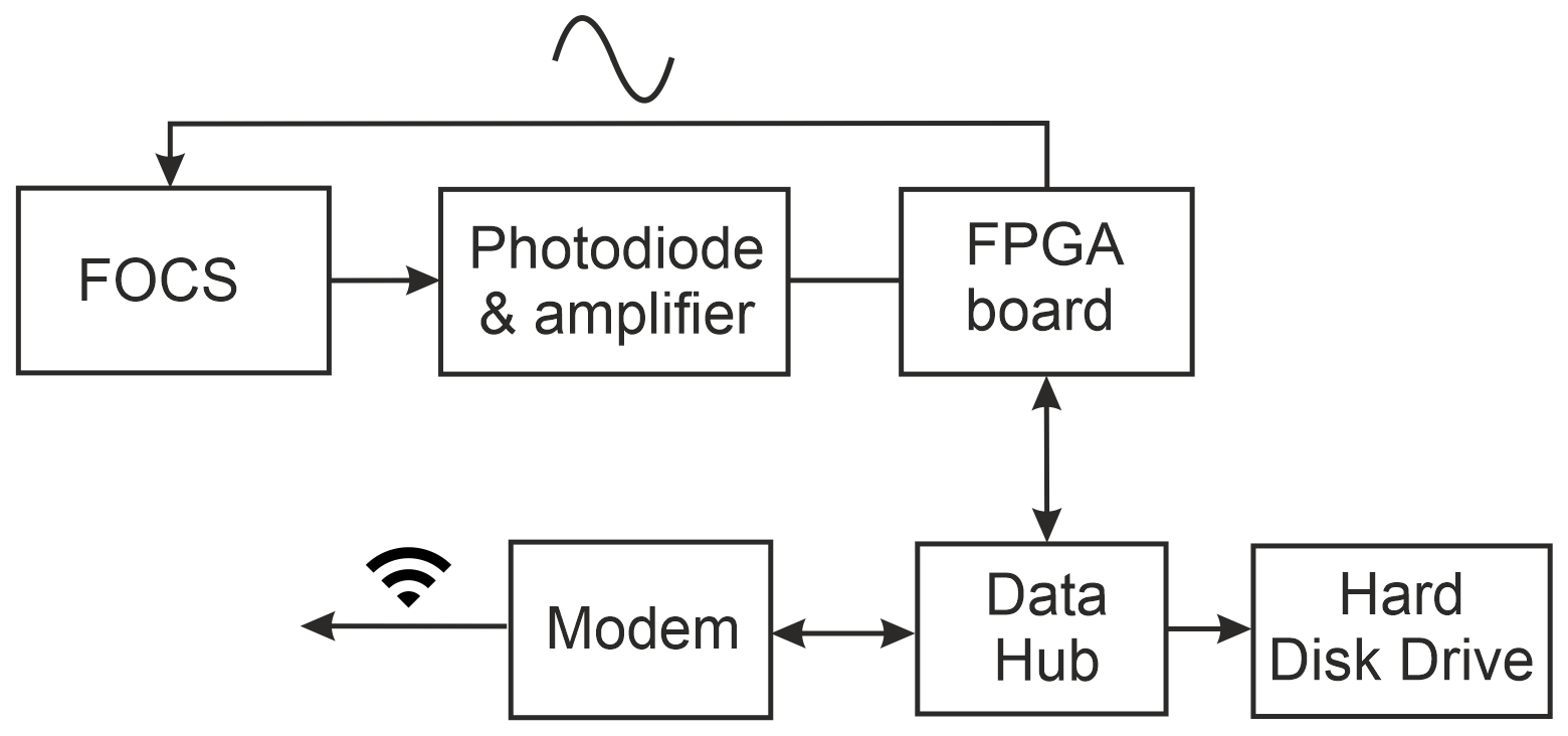
Figure 2 Block diagram of the electronic signal processing chain. The central elements in the electronics module are the FPGA board for signal extraction and sensor operation and the data hub for data storage and remote access.

3.2 Noise-equivalent current

To estimate the fundamental detection limit imposed by the optoelectronic detection circuit, we estimated the noise amplitudes for the presented sensor system, which limit its sensitivity. The current that would generate the same output signal as the sum of all noise sources, resulting in a signal-to-noise ratio of 1, can then be given as a figure of merit and is called the noise-equivalent current I_NE.

For the polarization-rotated reflection interferometer, the generated photocurrent i_d can be described by

$$\begin{array}{}\text{(4)}& i_d=r\left({\displaystyle \frac{P_{\mathrm{0}}}{\mathrm{2}}}(\mathrm{1}+\sin \mathit{\varphi })\right).\end{array}$$

Here, r relates to the conversion coefficient of the photo diode, which is usually 1 A W⁻¹ for InGaAs detectors at 1550 nm, and P₀=200 µW is the optical power measured at the output port of the circulator. Thus, the photo detector signal consists of a mean contribution $\langle i\rangle =\frac{r{P}_{\mathrm{0}}}{\mathrm{2}}$ and a variable term dependent on the Faraday phase shift $\frac{r{P}_{\mathrm{0}}}{\mathrm{2}}\sin \mathit{\varphi }$.

In FOCS, there are three uncorrelated noise sources. Thermal noise, or Johnson–Nyquist noise, concerns the thermal movement of electrons in the electric circuit. Photon shot noise, or Poisson noise, arises from the statistical fluctuations of the number of photons over time from the light source. Finally, light source intensity noise refers to the beating of spectral components at random phases (Bohnert, 2024).

The rms values of the individual noise sources in the signal can be given as

$$\begin{array}{}\text{(5)}& i_{\mathrm{th}}=\sqrt{{\displaystyle \frac{\mathrm{4}kT}{R_{\mathrm{L}}}}\mathrm{\Delta }f},i_{\mathrm{sh}}=\sqrt{\mathrm{2}e\langle i\rangle \mathrm{\Delta }f},i_{\mathrm{in}}=\sqrt{{\displaystyle \frac{\langle i{\rangle }^{\mathrm{2}}}{\mathrm{\Delta }{\mathit{\nu }}_{\mathrm{e}}}}\mathrm{\Delta }f}.\end{array}$$

Here, k is Boltzmann's constant, and T is the ambient temperature, assumed as 25 °C. R_L=22 kΩ denotes the resistance experienced by the photocurrent, while the detection bandwidth Δf is determined by the FPGA's Fourier transform algorithm, with a Fourier window bin size of f_b=4883 Hz = 2Δf. Furthermore, e is the electron charge, and $\mathrm{\Delta }{\mathit{\nu }}_{\mathrm{e}}=\mathrm{7.49}\times {\mathrm{10}}^{\mathrm{12}}$ Hz is the SLD's spectral width.

Using Eq. (1) and setting the variable term in Eq. (4) equal to the noise amplitudes in Eq. (5), the separate noise-equivalent currents follow for N=50:

$$\begin{array}{}\text{(6)}& {\displaystyle }{I}_{\mathrm{NE}}^{\left(\mathrm{th}\right)}={\displaystyle \frac{\mathrm{1}}{VNr{P}_{\mathrm{0}}}}\sqrt{{\displaystyle \frac{kT}{R_{\mathrm{L}}}}\mathrm{\Delta }f}=\mathrm{0.003}\mathrm{A},\text{(7)}& {\displaystyle }{I}_{\mathrm{NE}}^{\left(\mathrm{sh}\right)}={\displaystyle \frac{\mathrm{1}}{\mathrm{2}VN}}\sqrt{{\displaystyle \frac{e}{r{P}_{\mathrm{0}}}}\mathrm{\Delta }f}=\mathrm{0.019}\mathrm{A},\text{(8)}& {\displaystyle }{I}_{\mathrm{NE}}^{\left(\mathrm{in}\right)}={\displaystyle \frac{\mathrm{1}}{\mathrm{4}VN}}\sqrt{{\displaystyle \frac{kT}{R_{\mathrm{L}}}}\mathrm{\Delta }f}=\mathrm{0.1289}\mathrm{A}.\end{array}$$

Thermal noise and shot noise both decrease with increasing optical power. Since the noise sources are uncorrelated, the total noise-equivalent current is the sum of the squared individual contributions. To compare this figure of merit with other sensor systems, it is usually given independent of the measurement bandwidth Δf:

$$\begin{array}{}\text{(9)}& \begin{array}{rl}{I}_{\mathrm{NE}}& =\sqrt{(I_{\mathrm{NE}}^{\left(\mathrm{th}\right)}{)}^{\mathrm{2}}+(I_{\mathrm{NE}}^{\left(\mathrm{sh}\right)}{)}^{\mathrm{2}}+(I_{\mathrm{NE}}^{\left(\mathrm{in}\right)}{)}^{\mathrm{2}}}\\ & =\mathrm{0.1305}\mathrm{A}\widehat{=}\mathrm{2.64}\mathrm{mA}{\sqrt{\mathrm{Hz}}}^{-\mathrm{1}}.\end{array}\end{array}$$

It is evident that the dominant noise source in this case is intensity noise. A reduction in the overall noise level by using longer sampling times is not feasible due to the desired simultaneous measurement of AC and DC. We discuss the optimization of noise levels in Sect. 5.

4 Field measurements

4.1 Installation

Infield measurements with the presented FOCS system were carried out in Vienna, Austria, at an electrical substation of the local grid operator Austrian Power Grid AG. The aim was to compare the FOCS measurements on one phase of the electric grid to reference measurements performed by an existing zero-flux measurement system, which detects the total DC of all three phases in the transformer neutral point of the high-voltage side. At the selected 600 MVA 380/220 kV power transformer, significant DC loads have been recorded during periods of increased solar activity over recent years.

The developed FOCS system has exhibited sub-ampere DC resolution for expected AC loads during laboratory tests (Mandl et al., 2025). The derivation of small DC biases superimposed on AC signals from the FOCS output has been shown in previous work (Mandl et al., 2024). For the zero-flux CT, a current value is recorded every second, and the data are filtered with a cutoff frequency f_lim=0.5 Hz to keep the quasi-DC components. For comparison, the same filtering has been applied to the FOCS data.

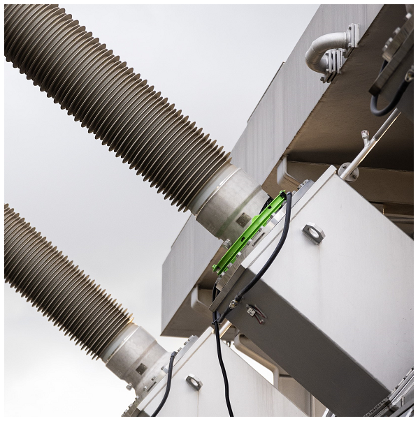
Figure 3 Installation of FOCS sensing head on one phase of a 380/220 kV power transformer in Vienna, Austria.

To fit the transformer bushing, a sensing head with a radius of R=24 cm was constructed and produced through additive manufacturing, resulting in N=50 spun fiber windings. The cabinet including the optical elements and the electronics module was mounted on ground level and connected to the sensing head via a PMF line (black tube in Fig. 3). The proper modulation frequency was calibrated after sensor installation by ensuring a vanishing first harmonic in the spectrum. To avoid spectral beating during demodulation, the modulation frequency f_m was set to an integer multiple of the FPGA board's Fourier window bin size, namely f_m = 463 867 Hz, resulting in a modulation depth of Δϕ₀=1.86.

4.2 Low-voltage measurements

The FOCS sensing head was first installed on phase b on the low-voltage side of the transformer, as shown in Fig. 4. The transformer is a YNyn0 type, which means that both neutral points are accessible. However, only the neutral point on the HV side is permanently grounded. For that configuration, the loop via the HV line and the neutral point to ground should not close, and therefore no geomagnetic direct current is expected to flow in phase b.

When considering GICs in HV networks, the measured DCs at the neutral point of the transformer are generally assumed to be evenly distributed across phases a, b, and c. However, in reality, this may not be the case, as the winding resistances of the transformers also differ slightly due to manufacturing tolerances, resulting in a lower or higher resistive path for the GICs in the individual phases.

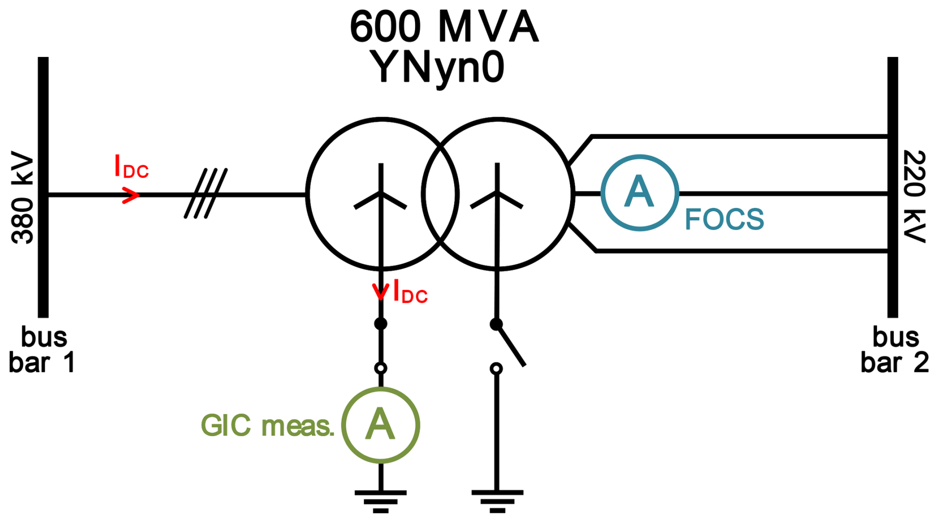
Figure 4 Schematic representation of the power transformer, in which the DC measurement is located at the neutral point of the high-voltage (bus bar 1) side and the FOCS measurement is located at phase b of the low-voltage side (bus bar 2).

Due to the different winding resistances of the transformers, this results in an unbalanced resistance bridge, and the induced DC flows between the two rigidly grounded transformers, with a small part of the DC also flowing through the transformer with the isolated neutral point, as shown in Fig. 5. For this reason, an induced DC may also be recorded by the FOCS measurement system on phase b, when operated as pictured in Fig. 4. To the best of our knowledge, the occurrence of GICs on the non-grounded transformer side has not been verified before.

According to the National Oceanic and Atmospheric Administration (NOAA), solar storms are categorized using the G1 to G5 space weather scale, which reflects increasing levels of intensity and potential impact (NOAA Space Weather Prediction Center, 2023). On 1 January 2025, a geomagnetic storm of class G3 was recorded. The zero-flux CT in the grounded transformer neutral recorded a maximum DC amplitude of $I_{\mathrm{ZF}}=-\mathrm{12.2}$ A. The FOCS showed a DC bias with a maximum amplitude of $I_{\mathrm{FOCS}}=-\mathrm{8.4}$ A, proving for the first time that GICs also flow on the non-grounded transformer side (Fig. 6). However, current amplitudes and dynamics may not be directly compared due to the different locations of the two sensors.

Since the FOCS is able to permanently record the AC signal, it is possible to reconstruct the original current waveform and perform a harmonic analysis. In power transformers, the presence of a DC bias shifts the operating point of the core into the nonlinear region of the B–H curve, leading to half-cycle saturation of the transformer core. This saturation manifests in an increase in the even harmonics of the 50 Hz AC signal, while one would recognize a humming sound close to the transformer (Baier, 2010). The reconstructed AC waveform was Fourier analyzed, with a window size of 1 s. Even harmonics up to the 10th order were extracted and filtered. Indeed, as shown in Fig. 7, an increase was recorded in even AC harmonics at the time of the DC maximum. As expected, the amplitudes of the harmonics add up to the determined DC value.

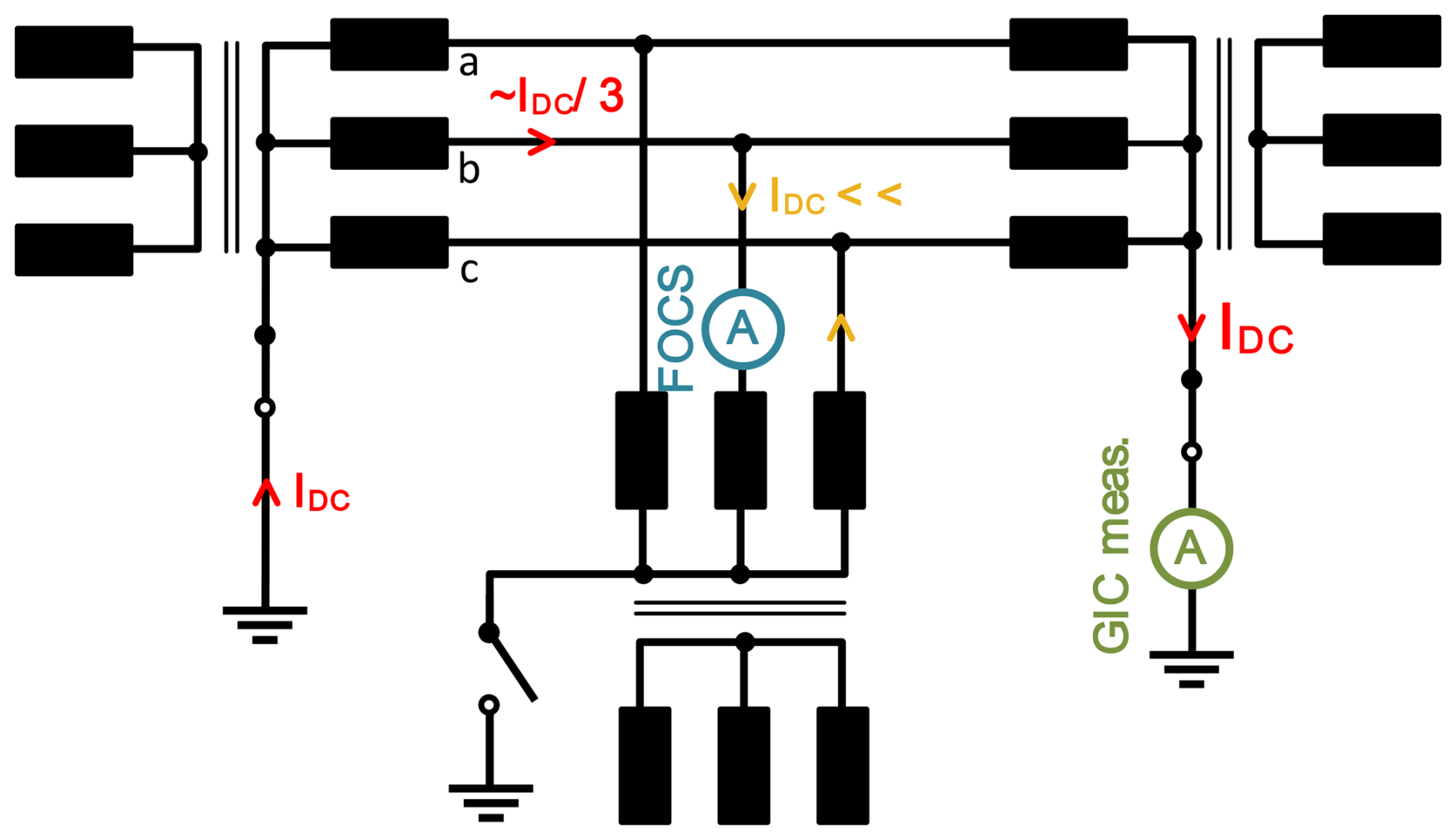
Figure 5 Equivalent circuit diagram of the transformer arrangement, in which two neutral points are grounded and a small part of the direct current flows through the third transformer.

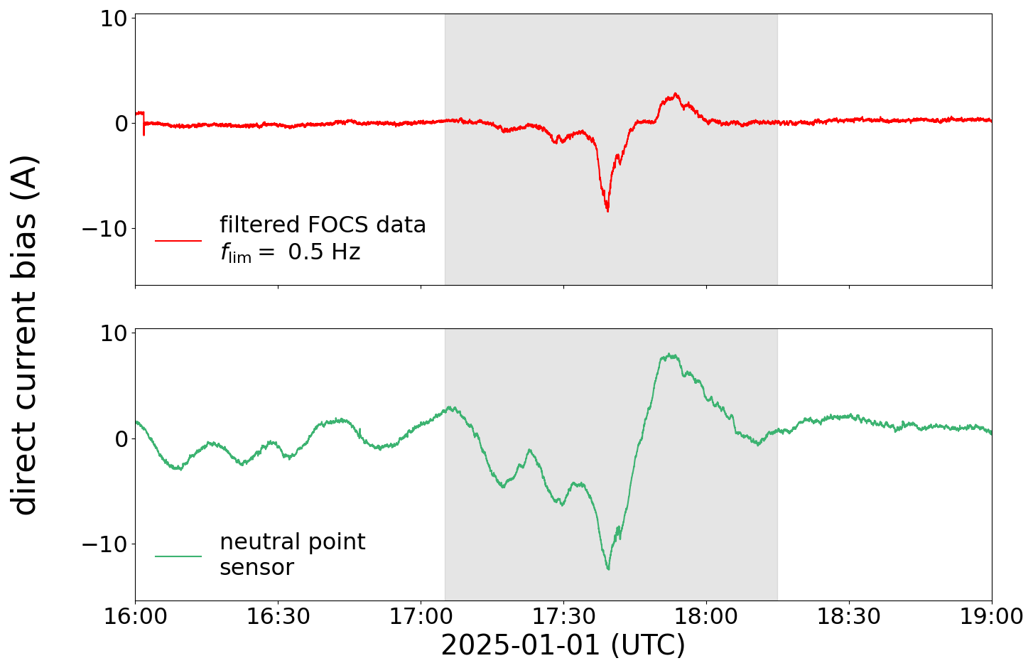
Figure 6 Comparison of FOCS and zero-flux CT data on 1 January 2025. The GIC event is shown in the gray area.

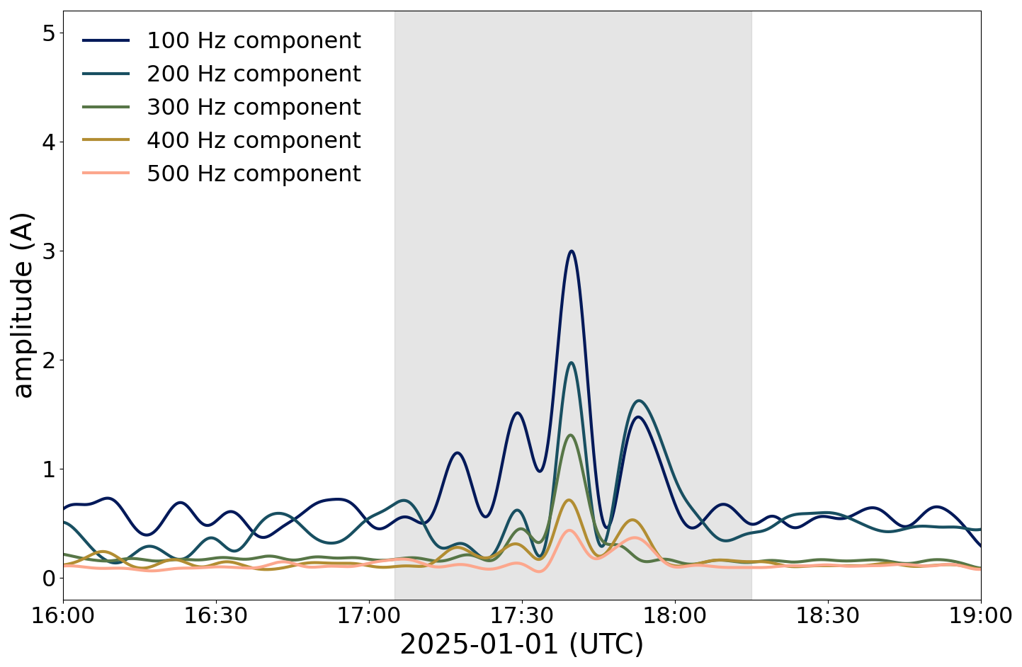
Figure 7 Amplitudes of even harmonics in the reconstructed AC signal on 1 January 2025, where f_lim=10 Hz. The GIC event is shown in the gray area.

4.3 High-voltage measurements

For a direct comparison with the reference zero-flux measurement, the FOCS was attached on phase b of the transformer's 380 kV high-voltage side, as shown schematically in Fig. 8. The predominant assumption, which has been supported by GIC simulations, is that the induced geomagnetic direct current is evenly distributed across the three phases a, b, and c and that therefore the FOCS measurement system should experience one-third of the total DC via the neutral point on the HV side.

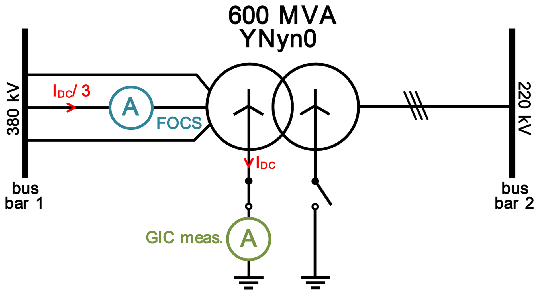
Figure 8 Schematic representation of the power transformer, in which the DC measurement is located at the neutral point of the high-voltage side and the FOCS measurement is located at phase b of the high-voltage winding (bus bar 1).

In the evening hours of 1 September 2025, a solar particle flare caused a geomagnetic storm of class G1. The zero-flux CT showed a maximum DC bias of $I_{\mathrm{ZF}}=-\mathrm{2.20}$ A. With the FOCS measurement system, a maximum DC amplitude of $I_{\mathrm{FOCS}}=-\mathrm{0.97}$ A was recorded (Fig. 9).

While the current measured by the FOCS is not exactly one-third of the total DC, it lies within the expected order of magnitude. Regarding the precision of the developed sensor, it has to be noted that the current magnitudes caused by the G1 storm are near the detection limit of the sensor reported in Mandl et al. (2025), which may also serve as an explanation for the reduced signal dynamic. Furthermore, after months of continuous operation, we noticed a constant DC offset in the retrieved current signal, which had to be accounted for during post-processing.

Again, a harmonic analysis of the AC waveform was performed. The amplitudes up to the sixth harmonic show an increase coinciding with the maximum DC bias (Fig. 10). However, the precision regarding the sum of the individual amplitudes equaling the total DC has degraded compared to Fig. 7.

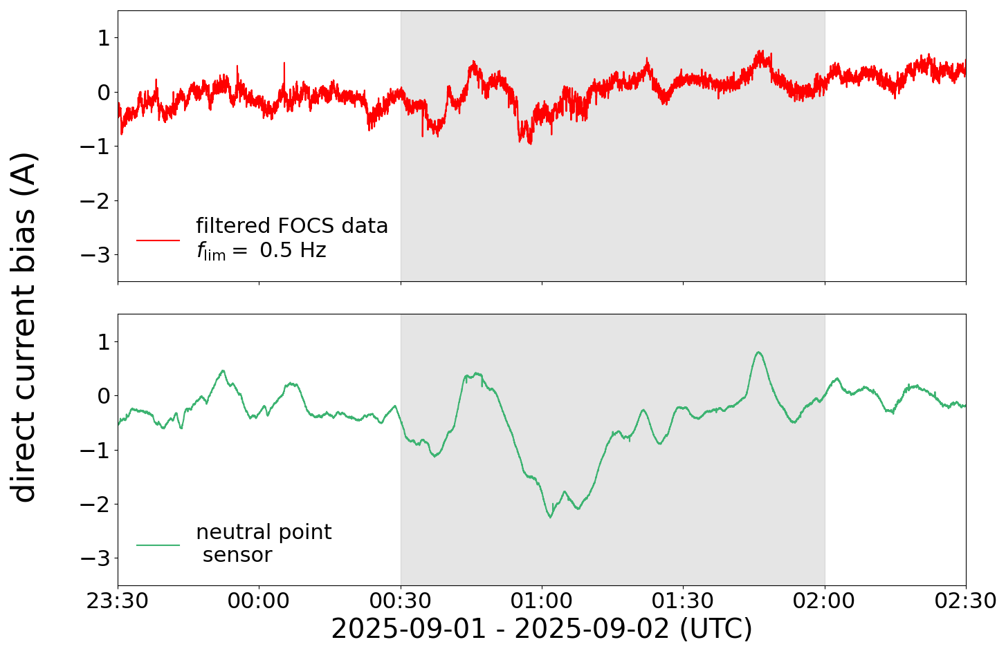
Figure 9 Comparison of FOCS and zero-flux CT data on 1–2 September 2025. The GIC event is shown in the gray area.

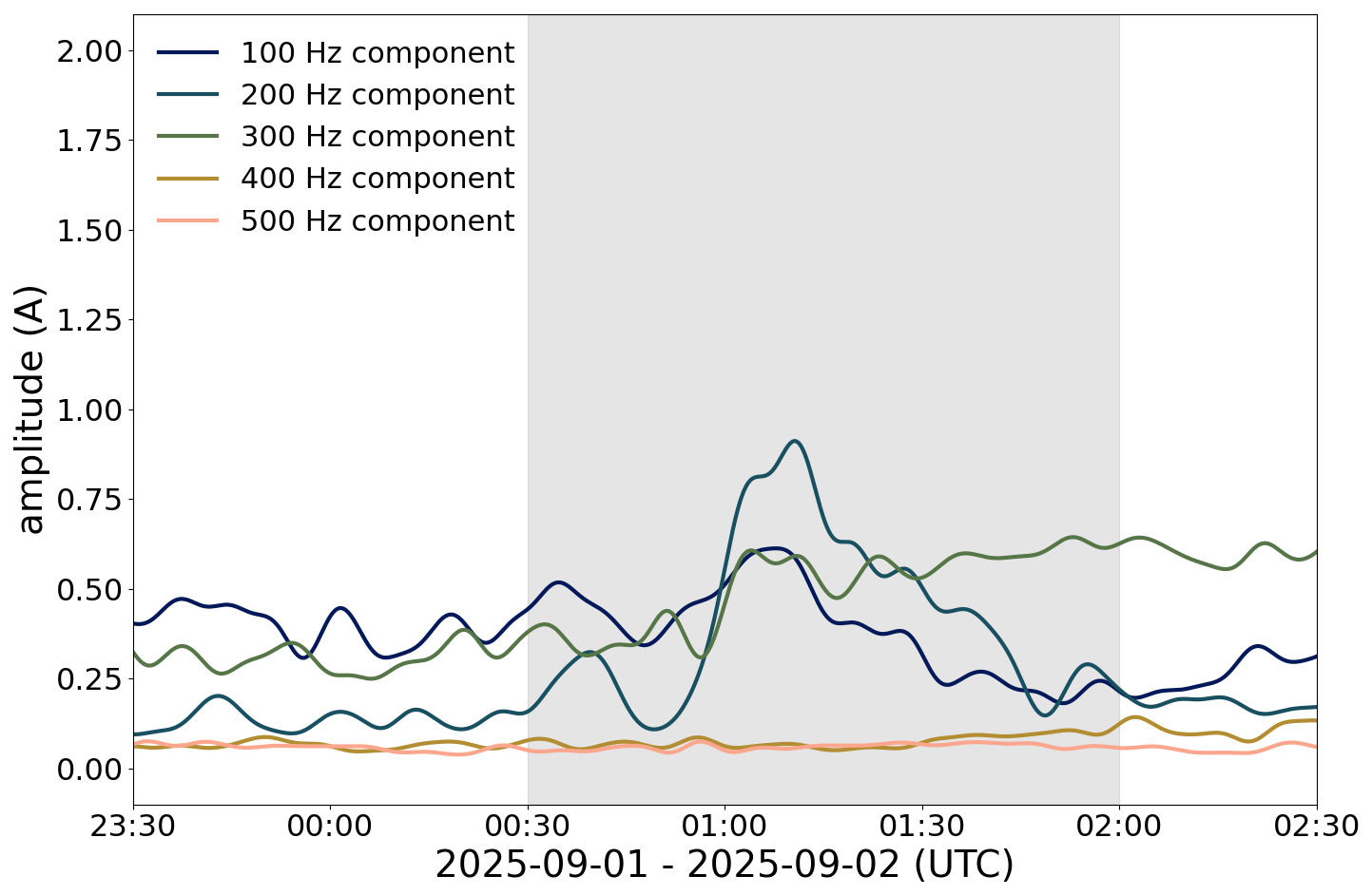
Figure 10 Amplitudes of even harmonics in the reconstructed AC signal on 1–2 September 2025, where f_lim=10 Hz. The GIC event is shown in the gray area.

5 Conclusions

Within this work, we have developed a fiber-optic current sensor capable of detecting small direct currents superimposed on an alternating-current signal on high-voltage potential. The system is equipped with an electronics module that records signals, post-processes data via FPGA, stores data, and allows remote data access for long-term monitoring.

We calculated the noise-equivalent current as a threshold sensitivity imposed by the optoelectronic detection circuit as $I_{\mathrm{NE}}=\mathrm{2.64}\mathrm{mA}{\sqrt{\mathrm{Hz}}}^{-\mathrm{1}}$, which is comparable to similar sensor systems (Laming and Payne, 1989; Gubin et al., 2006). During two geomagnetic events, we showed for the first time the occurrence of geomagnetically induced currents on the transformer's low-voltage side, as well as a first measurement of geomagnetically induced currents (GICs) on a single phase on HV potential. A harmonic analysis of the retrieved AC waveform proved the presence of direct currents via an increase in the even AC harmonics.

The noise floor of the detection may be improved by balancing the number of fiber windings N and the optical power P₀. By increasing N, intensity noise will be reduced, and the shot noise-dominated regime may be reached. However, adding more spun fiber increases the cost factor, while the transmitted optical power may be reduced, which would raise the thermal and shot noise components. We particularly suggest optimizing the factor $N\sqrt{P_{\mathrm{0}}}$ to keep the shot noise constant and find an acceptable trade-off.

The sensor data show an increasing DC offset after prolonged operation. Accelerated aging tests of FOCS components have indicated changed device characteristics over time and varying ambient conditions (Lenner et al., 2020). To prevent degradation in the sensor's performance, we suggest identifying the optimum operating point through continuously monitoring the recorded optical power as described in Mandl et al. (2024) and readjusting the modulation parameters accordingly. Another method that has shown improved long-term drift stability is operating the sensor in a closed-loop configuration with square-wave modulation (Lefevre, 2022).

Finally, for continuous infield operation, environmental influences on the sensing head should be taken into consideration by ensuring appropriate fiber packaging and the mitigation of temperature effects on the $\mathit{\lambda }/\mathrm{4}$ retarder and the sensing fiber.