Calibration of tri-axial MEMS accelerometers in the low-frequency range – Part 2: Uncertainty assessment

A comparison among three methods for the calibration of tri-axial accelerometers, in particular MEMS, is presented in this paper, paying attention to the uncertainty assessment of each method. The first method is performed according to the ISO 16063 standards. Two innovative methods are analysed, both suitable for in-field application. The effects on the whole uncertainty of the following aspects have been evaluated: the test bench performances in realizing the reference motion, the vibration reference sensor, the geometrical parameters and the data processing techniques. The uncertainty contributions due to the offset and the transverse sensitivity are also studied, by calibrating two different types of accelerometers, a piezoelectric one and a capacitive one, to check their effect on the accuracy of the methods under comparison. The reproducibility of methods is demonstrated. Relative uncertainty of methods ranges from 3 to 5 %, depending on the complexity of the model and of the requested operations. The results appear promising for low-cost calibration of new tri-axial accelerometers of MEMS type.

1 Introduction

Among the many examples that can be found in the literature, showing the industrial and scientific interest into calibration of tri-axial accelerometers, particular attention should be paid to works dealing with vibrations in the low-frequency range (Garg and Schiefer, 2017) and with accelerometers of the MEMS technology (Schrab and Ebadollahi, 2017; Ye et al., 2017; Goryanina and Lukyanov, 2017; Kulhanek and Skuta, 2017). In fact, both topics present many aspects to be faced and solved by means of improved solutions with respect to the available ones.

The main problems of low-frequency (0.2 to 6 Hz) accelerometer calibration are of two types (Garg and Schiefer, 2017): low acceleration amplitude, so that a high noise to signal ratio occurs with increased uncertainty, and the need to use long stroke linear shakers, which are expensive if high calibration accuracy has to be achieved, and not easy to use in-field.

The wide interest in MEMS technology derives from the capability of these sensors to offer the possibility of obtaining sensors of very low cost able to get promising measuring performances, even though many interfering effects have to be taken into account in the design, production and application phases. An example is the possibility of developing procedures that could be implemented both on-line and in-line (D'Emilia et al., 2018). In the authors' view, in-line calibration refers to the possibility of calibrating during assembly in industrial processes, for continuous monitoring and controlling of processes. On-line calibration refers to the calibration of sensors installed on an industrial plant, directly carried out on the production line to be monitored without moving it to a laboratory. For these reasons, many improvements are proposed in order to reduce the effects of non-linearities (Schrab and Ebadollahi, 2017), of transversal sensitivities (Yuan et al., 2015; Jianyan et al., 2015), to improve the accuracy of data processing techniques (Ye et al., 2017; Goryanina and Lukyanov, 2017; Kulhanek and Skuta, 2017). Compensation of interfering effects is demonstrated and/or reduction of uncertainty, even though a big issue arises in most of these contributions, referring to the traceability of results and of the procedure to standard methods, as extensively discussed in Garg and Schiefer (2017).

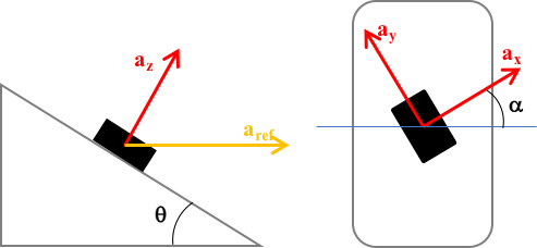
Figure 1 Geometrical representation of angles, with respect to the reference acceleration (a_ref).

Figure 2 Test bench – scheme.

In D'Emilia et al. (2018), intended as Part 1 of the present paper, the authors proposed a comparison among three methods, with the aim of presenting calibration procedures for tri-axial accelerometers of different types able to merge requirements of in-field operability, like low cost and simplicity of operation, better than a reference method, to the possibility of easily checking the traceability to reference (D'Emilia et al., 2011). In fact, one of the methods under examination adopts many of the issues of the reference methods (ISO 16063-1:1998; ISO 16063-11:1999; ISO 16063-21:2003; ISO 16063-31:2009).

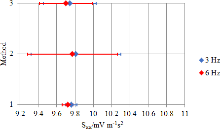
Figure 3 Piezo-electric accelerometer: comparison between methods (main sensitivity along the x axis, S_xx).

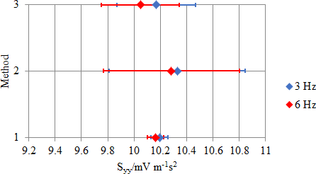
Figure 4 Piezo-electric accelerometer: comparison between methods (main sensitivity along the y axis, S_yy).

Figure 5 Piezo-electric accelerometer: comparison between methods (main sensitivity along the z axis, S_zz).

Part 1 (D'Emilia et al., 2018) explains the motivations of introducing new methods and outlines pros and cons of both with respect to an in-field exploitation of each one; this paper aims to check the compatibility of results of methods, by a detailed and motivated assessment of uncertainty of methods to be compared.

Uncertainty assessment is carried out according to the detailed analysis of the measurement model, with particular attention given to the main uncertainty contributions. This not only allows us to define the uncertainty budget of each method, but also to understand the practical motivations that address the use of each method with reference to a specified application, depending on situations. In fact, a particular field of application can be identified.

Section 2 of the paper is devoted to the short presentation of the methods to be compared and the test bench, where comparison has been carried out. This will allow us to understand the main uncertainty causes and their effect, and also the way the issue of traceability is satisfied. In Sect. 3 the budget of uncertainty for each method is discussed and presented, together with the model of uncertainty propagation. The main results concerning the reproducibility of results are discussed in Sect. 4. Conclusions end the paper.

2 Calibration methods

The methods of calibration are described in detail in D'Emilia et al. (2018).

The principal characteristics of each method, useful for the uncertainty assessment, are described in the following.

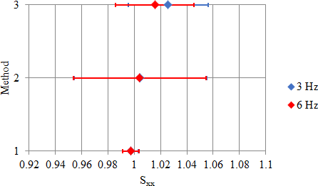
Figure 6 MEMS accelerometer: comparison between methods (main sensitivity along the x axis, S_xx).

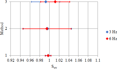
Figure 7 MEMS accelerometer: comparison between methods (main sensitivity along the y axis, S_yy).

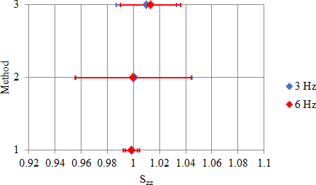
Figure 8 MEMS accelerometer: comparison between methods (main sensitivity along the z axis, S_zz).

2.1 Method 1

Each axis of the tri-axial sensor is excited along its direction. In this way, six transverse sensitivities can be calculated (S_xy, S_xz, S_yx, S_yz, S_zx, S_zy), in addition to the main ones (S_xx, S_yy, S_zz), which express the effect of the acceleration along a single axis, with respect to the other ones.

In particular, for example, when x axis is excited, the main sensitivity is calculated as Eq. (1), while the transverse sensitivities S_yx and S_zx are evaluated as Eqs. (2) and (3):

$$\begin{array}{}\text{(1)}& {\displaystyle }& {\displaystyle }{S}_{xx}={\displaystyle \frac{V_x}{a_x}},\text{(2)}& {\displaystyle }& {\displaystyle }{S}_{yx}={\displaystyle \frac{V_y}{a_x}},\text{(3)}& {\displaystyle }& {\displaystyle }{S}_{zx}={\displaystyle \frac{V_z}{a_x}},\end{array}$$

where V_x, V_y and V_z are the amplitudes of the x, y and z outputs of the accelerometer under test, and a_x is the amplitude of the reference signal in the x direction.

2.2 Method 2

Method 2 involves the simultaneous excitation of the three axes of the accelerometer under test. For this purpose, the accelerometer is mounted onto the surface of a clamp, inclined at an angle θ = 35^∘ with respect to the horizontal plane on which the motion is realized; furthermore, the accelerometer is rotated on the clamp surface with an angle α = 45^∘, in order to excite the three axes in the same way, with a single horizontal sinusoidal acceleration. Angles θ and α are according to Fig. 1.

The reference accelerations along the three axes can be obtained as Eqs. (4), (5) and (6):

$$\begin{array}{}\text{(4)}& {\displaystyle }& {\displaystyle }{a}_x\left(t\right)=-a_{\mathrm{ref}}\left(t\right)\cdot \cos \left(\mathit{\theta }\right)\cdot \sin \left(\mathit{\alpha }\right),\text{(5)}& {\displaystyle }& {\displaystyle }{a}_y\left(t\right)=-a_{\mathrm{ref}}\left(t\right)\cdot \cos \left(\mathit{\theta }\right)\cdot \cos \left(\mathit{\alpha }\right),\text{(6)}& {\displaystyle }& {\displaystyle }{a}_{\mathrm{z}}\left(t\right)=a_{\mathrm{ref}}\left(t\right)\cdot \sin \left(\mathit{\theta }\right),\end{array}$$

where a_ref(t) is the time-varying acceleration in the motion direction, measured by a reference sensor.

The output signal and the reference one are analysed by the fast Fourier transform in correspondence to the oscillation frequency, with the purpose to evaluating their spectral amplitudes. The constant terms, gravity dependent, do not affect the results.

This approach does not allow us to calculate the transverse sensitivities, since similar acceleration components are realized along all axes, simultaneously, without the possibility of extracting the effect of transverse sensitivities. A periodic verification is necessary that the transverse sensitivities are negligible (< 5 % with respect to the main sensitivities).

2.3 Method 3

Method 3 (D'Emilia et al., 2015, 2016a, b) is based on the following model, describing the relation between the input accelerations and the output signals as in Eq. (7):

$$\begin{array}{}\text{(7)}& \left(\begin{array}{l}{V}_x\\ V_y\\ V_z\end{array}\right)=\left(\begin{array}{lll}{S}_{xx}& S_{xy}& S_{xz}\\ S_{yx}& S_{yy}& S_{yz}\\ S_{zx}& S_{zy}& S_{zz}\end{array}\right)\cdot \left(\begin{array}{l}{a}_x\\ a_y\\ a_z\end{array}\right)+\left(\begin{array}{l}{q}_x\\ q_y\\ q_z\end{array}\right),\end{array}$$

where V = (V_i) is the output array, A = (a_i) is the reference acceleration array, S = (S_ij) is the sensitivity matrix and Q = (q_i) represents the offset array.

Then, a total of 12 parameters (main sensitivities, transverse sensitivities and offsets) are evaluated; a linear least-squares optimization (LSO) is used to estimate them (D'Emilia et al., 2015, 2016a, b). Then, this method simultaneously estimates not only the main sensitivities, but also the transverse ones and the offsets.

To avoid dependence among the input data for the LSO, the sensor is positioned in different angular positions with respect to the motion direction (four different angular positions).

The reference accelerations along the three axes can be obtained from Eqs. (8), (9), and (10), where g is the gravity acceleration, and a_ref(t) is the acceleration in the motion direction and measured by a reference sensor.

$$\begin{array}{}\text{(8)}& {\displaystyle }& {\displaystyle }{a}_x\left(t\right)=-a_{\mathrm{ref}}\left(t\right)\cdot \sin \left(\mathit{\alpha }\right)\cos \left(\mathit{\theta }\right)-g\cdot \sin \left(\mathit{\theta }\right)\cdot \sin \left(\mathit{\alpha }\right)\text{(9)}& {\displaystyle }& {\displaystyle }{a}_y\left(t\right)=-a_{\mathrm{ref}}\left(t\right)\cdot \cos \left(\mathit{\alpha }\right)\cdot \cos \left(\mathit{\theta }\right)-g\cdot \sin \left(\mathit{\theta }\right)\cdot \cos \left(\mathit{\alpha }\right)\text{(10)}& {\displaystyle }& {\displaystyle }{a}_z\left(t\right)=a_{\mathrm{ref}}\left(t\right)\cdot \sin \left(\mathit{\theta }\right)-g\cdot \cos \left(\mathit{\theta }\right)\end{array}$$

2.4 Test bench

For the comparison among calibration methods, two different accelerometers have been considered (D'Emilia et al., 2018):

• a MEMS accelerometer with a capacitive transduction system, with digital output (nominal sensitivity of the order of 1, dimensionless);

• a piezoelectric accelerometer with analogue output (nominal sensitivity of the order of 10 mV m⁻¹ s²).

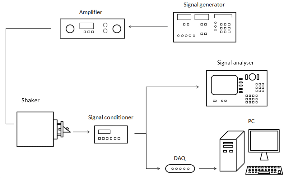
The test bench used is a vibrating table with a horizontal linear slide, the APS 113 ELECTRO-SEIS shaker. It is a long-stroke, electro-dynamic force generator, specifically suitable for low-frequency vibration testing. The slide is moved according to a sinusoidal law. A schematic representation of the test bench is depicted in Fig. 2.

In Method 1 the accelerometer is fixed directly on the horizontal vibrating table, with one of the three axes parallel to the motion direction. All three axes are tested in this way, recursively.

In methods 2 and 3 an inclined steel clamp is fixed on the vibrating table; the inclination angle θ is 35^∘ with respect to the horizontal plane. The inclined steel clamp allows a single angle α (Method 2) or multiple angles α (Method 3) to be obtained.

The motion of the vibrating table is accurately monitored by a laser Doppler vibrometer (LDV), as depicted in Fig. 1b.

The amplitude of the reference acceleration signal is obtained by applying Eq. (11), ω being the pulsation of the sinusoidal motion and v_vib the velocity measured by the LDV:

$$\begin{array}{}\text{(11)}& a_{\mathrm{ref}}=\mathit{\omega }\cdot v_{\mathrm{vib}}.\end{array}$$

The data acquisition system (DAQ) used is the NI USB-4431 by National Instruments. The module consists of a single analogue output and four analogue input channels for reading (one is connected to the LDV and the other three to the output of the piezo-electric accelerometer under test); each channel is equipped with antialiasing filters. The MEMS accelerometer is digitally connected to a computer, via a standard USB port. The output indicates the acceleration in engineering units.

The output channel drives the vibrating table. LabVIEW software is used for DAQ signal acquisition.

3 Uncertainty assessment

For the uncertainty assessment of the main sensitivities, evaluated by the calibration methods under analysis, the following contributions have been considered for methods 1, 2 and 3.

• Repeatability: random effect in repeat measurements; experimental standard deviation of arithmetic mean (ISO 16063-11:1999)

• Reproducibility: random effect in repeat measurements including mounting and dismounting

• Transversal acceleration of the bench: uncertainty due to transverse, bending and rocking acceleration on accelerometer output voltage measurement. According to ISO 16063-11:1999, they are considered sufficiently small to prevent excessive effects on the calibration results.

• Distortion: effect of total distortion on accelerometer output voltage measurement (ISO 16063-11:1999)

• Conditioner stability: effect of the signal conditioner, instability of reference amplifier gain, and effect of source impedance on gain

• Velocity error: effect of motion disturbance on velocity measurement

• Voltage: accelerometer output voltage measurement (waveform recorder; e.g. DAC/ADC resolution; voltmeter)

• Amplifier noise: effect of voltage disturbance on velocity measurement (e.g. hum and noise)

• Temperature: effect of temperature and other environmental effects on the behaviour of the transducer

In fact, these contributions depend on the mechanical characteristics of the test bench, on the reference and on the measuring chain components used in the tests.

In addition, for methods 2 and 3, two contributions, due to the uncertainty of the positioning angles α and θ, have to be taken into account:

• angle α;

• angle θ.

It has to be noticed that, in the case of Method 1, the uncertainty of the positioning angle (90^∘) is negligible and will not be considered.

Method 2 disregards the presence of transverse sensitivities in the calculation of the main ones; therefore, the following contribution is taken into account:

• transversal sensitivities: the contribution due to the effect of interferences between axes has to be considered. In fact, the experimental set-up of Method 2 realizes acceleration components on the axes contemporaneously.

For Method 3, the simultaneous estimates of the sensitivity matrix and of the offset vector by LSO are not completely independent between each other; therefore, the following contribution is considered in this case:

• offset effect: the uncertainty contribution due to the correlation effect between uncertainty on sensitivity terms and offset ones is considered.

Table 1 Uncertainty budget.

n/a: not applicable.

About the evaluation of the effect of the uncertainties of angles α and θ, the following considerations can be listed.

• Keeping Eqs. (4), (5) and (6) in mind, it can be noticed that the z axis is not dependent on the angle α, unlike the x and y axes. With the aim of evaluating the uncertainty of the main sensitivities related to the uncertainty of the angle α, the following equations can be written with reference to the x axis (for the y axis, the approach is the same):

  $$\begin{array}{}\text{(12)}& {\displaystyle }{S}_{xx}={\displaystyle \frac{V_x}{a_{\mathrm{ref}}}}\cdot \cos \left(\mathit{\theta }\right)\cdot \sin \left(\mathit{\alpha }\right),\end{array}$$

  where V_x and a_ref are the amplitudes of the corresponding signals. Applying the uncertainty propagation formula (JCGM 100:2008), except for the sign, we have

  $$\begin{array}{}\text{(13)}& {\displaystyle }u\left(S_{xx}\right)={\displaystyle \frac{V_x}{a_{\mathrm{ref}}\cdot \cos \left(\mathit{\theta }\right)}}\cdot \left({\displaystyle \frac{\mathrm{1}}{\sin (\mathit{\alpha }{)}^{\mathrm{2}}}}\right)\cdot \cos \left(\mathit{\alpha }\right)\cdot u\left(\mathit{\alpha }\right).\end{array}$$

  In particular, when α = 45^∘ (Method 2), then sin(α) = cos(α) and

  $$\begin{array}{}\text{(14)}& {\displaystyle }u\left(S_{xx}\right)={\displaystyle \frac{V_x}{a_{\mathrm{ref}}\cdot \cos \left(\mathit{\theta }\right)}}\cdot {\displaystyle \frac{\mathrm{1}}{\sin \left(\mathit{\alpha }\right)}}\cdot u\left(\mathit{\alpha }\right)=S_{xx}\cdot u\left(\mathit{\alpha }\right).\end{array}$$

  The same model for the uncertainty propagation has been assumed for Method 2 and Method 3, although some differences arise due to the transverse sensitivity effect and offset terms considered by Method 3, Eq. (7). Generally, these terms are not remarkable. Differences between methods must be considered as for the uncertainty propagation, in case of significant transverse sensitivities (> 10 %). This has been checked by means of numerical simulation.

  The variability on angle α was estimated to be 1.2^∘ = 0.021 rad: assuming a rectangular distribution, the corresponding relative standard uncertainty on the main sensitivity is equal to 1.2 % for Method 2. Method 3 considers repeated measurements at different α (at least 4). For this reason, the uncertainty on α has been reduced due to the random compensation effect, being equal to 1.0^∘, corresponding to a relative standard uncertainty on the main sensitivity equal to 1.0 %.

• Regarding the effect of the uncertainty of the angle θ, applying the uncertainty propagation formula to Eq. (8), except for the sign, we have

  $$\begin{array}{}\text{(15)}& {\displaystyle }u\left(S_{xx}\right)={\displaystyle \frac{V_x}{a_{\mathrm{ref}}\cdot \sin \left(\mathit{\alpha }\right)}}\cdot \left({\displaystyle \frac{\mathrm{1}}{\cos (\mathit{\theta }{)}^{\mathrm{2}}}}\right)\cdot \sin \left(\mathit{\theta }\right)\cdot u\left(\mathit{\theta }\right),\end{array}$$

  with θ = 35^∘:

  $$\begin{array}{}\text{(16)}& {\displaystyle }u\left(S_{xx}\right)=S_{xx}\cdot {\displaystyle \frac{\sin \left(\mathit{\theta }\right)}{\cos \left(\mathit{\theta }\right)}}\cdot u\left(\mathit{\theta }\right)=S_{xx}\cdot \mathrm{0.70}\cdot u\left(\mathit{\theta }\right).\end{array}$$

  The variability on angle θ was estimated to be 0.30^∘ = 0.0052 rad: assuming a rectangular distribution, the corresponding relative standard uncertainty on the main sensitivity is equal to 0.21 %.

  Similarly, with regards to the z axis, the corresponding relative standard uncertainty on the main sensitivity is equal to 0.42 %, according to the following:

  $$\begin{array}{ll}{\displaystyle }u\left(S_{zz}\right)& {\displaystyle }={\displaystyle \frac{V_z}{a_{\mathrm{ref}}}}\cdot \left({\displaystyle \frac{\mathrm{1}}{\sin {\left(\mathit{\theta }\right)}^{\mathrm{2}}}}\right)\cdot \cos \left(\mathit{\theta }\right)\cdot u\left(\mathit{\theta }\right)\\ \text{(17)}& {\displaystyle }& {\displaystyle }=S_{zz}\cdot {\displaystyle \frac{\cos \left(\mathit{\theta }\right)}{\sin \left(\mathit{\theta }\right)}}\cdot u\left(\mathit{\theta }\right)=S_{zz}\cdot \mathrm{1.4}\cdot u\left(\mathit{\theta }\right).\end{array}$$

About the evaluation of the effect of transversal sensitivities on Method 2, the following considerations can be listed.

• From Eq. (7),

  $$\begin{array}{}\text{(18)}& {\displaystyle }{V}_x=S_{xx}\cdot a_x+S_{xy}\cdot a_y+S_{xz}\cdot a_z.\end{array}$$

  Then, the main sensitivity S_xx can be obtained as

  $$\begin{array}{}\text{(19)}& {\displaystyle }{S}_{xx}={\displaystyle \frac{V_x}{a_x}}-S_{xy}\cdot {\displaystyle \frac{a_y}{a_x}}-S_{xz}\cdot {\displaystyle \frac{a_z}{a_x}}.\end{array}$$

  a_x = a_y = a_z in the experimental bench being used for Method 2, it can be written as

  $$\begin{array}{}\text{(20)}& {\displaystyle }{S}_{xx}={\displaystyle \frac{V_x}{a_x}}-S_{xy}-S_{xz}.\end{array}$$

  Therefore, the main sensitivity S_xx, obtained as a ratio between V_x and a_x, should be corrected for transverse sensitivities S_xy and S_xz: the correction is not applied, but these terms will be considered in the uncertainty budget for Method 2.

  It can be noticed that the terms of bias, which likewise are not determined by Method 2, do not affect the calculation of the main sensitivities, because the method is based on a FFT analysis at the frequency of interest only.

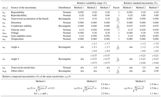
The uncertainty budgets for methods 1, 2 and 3 are shown in Table 1.

4 Results

Figures 3, 4, 5 and 6, 7, 8 show the comparison for the main sensitivities as evaluated by all methods for the piezoelectric sensor and the MEMS one, respectively. Sensitivity is in millivolt per metre second squared (mV m⁻¹ s²), for the piezo-electric accelerometer, while it is dimensionless for the MEMS accelerometer, since the digital output values are directly expressed in metre per second squared (m s⁻²).

In all cases, the expanded uncertainties, according to previous evaluations (k = 2), are represented by error bars.

The main observations concerning the results are as follows.

• The methods offer reproducible results, since differences among the three methods are negligible with respect to their uncertainties.

• The main contributions to the uncertainty budget for each method have been identified and quantitatively evaluated, leading to the following estimates of the whole uncertainty, for each measuring axis.

  • Method 1 is of the order of 0.6 % for all axes.

  • Method 2 is of the order of 5 % for all axes.

  • Method 3 is of the order of 3 % for all axes.

• Method 1 has been intended as the reference method.

• Method 2 is suitable for application, if transversal sensitivities and their effect are negligible.

• Method 3 allows the evaluation of transversal sensitivity and of offset terms; therefore, if these effects are remarkable, they can be estimated and do not affect the precision of the calibration.

The most suitable field of application of each method is extensively discussed in D'Emilia et al. (2018).

5 Conclusions

A comparison of three methods for calibration of tri-axial accelerometers, in particular MEMS, has been presented and attention is paid to the uncertainty assessment of each method. Method 1 is intended as an adjustment of standard procedures to get a traceable reference. Methods 2 and 3 are new methods, different for capability of taking into account the effect of offset terms and of transverse sensitivities, but both suitable for in-field application. The effects on the whole uncertainty of the test bench performances in realizing the reference motion, of the vibration reference sensor, which is a high accuracy vibrometer, of the geometrical parameters and of the data processing techniques, have been evaluated. For each method, the main contributions to the measurement uncertainty have been identified in order to define their most suitable field of application. The calibration of different type of accelerometers, piezoelectric and capacitive, is also used to check the effect of offset and transverse sensitivities on the accuracy of methods under comparison. Reproducibility of methods is demonstrated. Relative uncertainty of methods ranges from 3 to 5 %, depending on the complexity of model and of the requested operations. The results appear promising for low-cost calibration of new tri-axial accelerometers of MEMS type.