Dynamic characterization of multi-component sensors for force and moment

An improved set-up for the characterization of multi-component sensors for force and moment is presented. It aims at calibrating such sensors under continuous sinusoidal excitation. Special focus is put on the design of load masses and adapting elements to activate uniaxial force and moment components where possible. To identify the motion and acceleration of the load mass with 6 degrees of freedom, a photogrammetric measurement system is implemented in the existing set-up. Using the set-up described, different experiments are performed to analyse a commercial multi-component sensor and perform a parameter identification for its force components.

1 Introduction

The calibration and characterization of sensors for force and moment are typically performed in a static manner (DIN 51309, 2005; ISO 376, 2011). The dynamic behaviour of these sensors may differ significantly from the static behaviour. Especially the sensitivity coefficient, which is necessary to transform the sensor output signal into a force or moment signal, is subject to changes with higher frequencies of the dynamic excitation (Schlegel et al., 2012; Vlajic and Chijioke, 2016). Therefore, if such sensors are to be used in a dynamic environment, their dynamic behaviour needs to be analysed (Bartoli et al., 2012). For force and acceleration sensors, typical characterization methods are sinusoidal excitation (Schlegel et al., 2012) and shock excitation (Bruns et al., 2002). Torque sensors are currently evaluated under sinusoidal excitation (Klaus, 2016).

The aforementioned calibration approaches are limited to uniaxial sensors or calibrations of only one axis of multiaxial or multi-component sensors (MCSs). Such MCSs have become more popular in the last few years, which has resulted in the need for new calibration procedures (Baumgarten et al., 2016; Kim, 2000; Nitsche et al., 2017a). Challenges in the calibration of MCSs are, among other things, the generation of forces and moments with defined directions, the identification of the force and moment vector in a reference system (Röske et al., 2001) and the alignment of sensor and reference coordinate systems (Nitsche et al., 2017b).

For the dynamic calibration of MCSs, very few approaches exist. Park et al. (2008) deployed an electrodynamic shaker set-up with a vertical excitation direction at the Physikalisch-Technische Bundesanstalt (PTB) using different adapting elements to activate sinusoidal excitations in different directions. Schleichert et al. (2016) designed a fixed sensor frame with different adapting directions for an electrodynamic plunger actuator. In both set-ups, the reference force can only be calculated in the direction of excitation. Additional components like rocking modes cannot be detected.

In the following sections, an improved set-up for the dynamic analysis of MCSs is described. The force generation is based on the periodic acceleration of a load mass connected to an MCS. The theory behind sinusoidal calibration is explained using the example of uniaxial force calibration in Sect. 2. The improved set-up includes a specially designed load mass and a three-dimensional acceleration reference based on photogrammetry. Section 3 summarizes the new set-up. A dynamic model of an MCS is described in Sect. 4. Finally, the parameters of the model are identified from experimental data as described in Sect. 5.

2 Sinusoidal calibration of force and moment sensors

The aim of the dynamic calibration of force and moment sensors is the identification of the parameters needed to describe the dynamic behaviour and the sensitivity coefficient as a function of the excitation frequency (Schlegel et al., 2012). The typical model used for the description of such a sensor is a mass-spring-damper system. The parameters needed to describe this model are the spring constant k_z, the damping parameter b_z and the mass m (Fig. 1). The mass m is composed of the external load mass m_e, the mass of adapting elements m_a and the internal moving mass of the sensor m₁.

Figure 1 Dual-mass oscillator as a model for uniaxial force sensors.

From the given parameters, the dynamic sensitivity S can be calculated according to Schlegel et al. (2012):

$$\begin{array}{}\text{(1)}& S={\displaystyle \frac{c}{\sqrt{k_z^{\mathrm{2}}+(b_z\mathit{\omega }{)}^{\mathrm{2}}}}}\approx {\displaystyle \frac{c}{k_z}}\left(\mathrm{1}-{\displaystyle \frac{\mathrm{1}}{\mathrm{2}}}{\left({\displaystyle \frac{b_z}{k_z}}\right)}^{\mathrm{2}}{\mathit{\omega }}^{\mathrm{2}}\right),\end{array}$$

with c as a factor for unit conversion with the unit U m⁻¹ (U as a sensor signal unit, e.g. mV V⁻¹ for strain gauge sensors). In addition to the sensitivity S, the phase shift φ_s between the excitation and the sensor output can be calculated as follows:

$$\begin{array}{}\text{(2)}& {\mathit{\phi }}_{\mathrm{s}}\approx -{\displaystyle \frac{b_z}{k_z}}\mathit{\omega }.\end{array}$$

Both Eqs. (1) and (2) are approximations for a stiff coupling of the top mass to the sensor, which allows the influence of an additional spring-damper system describing the coupling to be neglected.

As an alternative to identifying the model parameters k and b, the dynamic sensitivity can be calculated as the ratio of the sensor signal output U and the acting dynamic force F (Park et al., 2008):

$$\begin{array}{}\text{(3)}& S={\displaystyle \frac{U}{F}}.\end{array}$$

In this case, only the moving mass m and its acceleration a are needed to calculate the acting force:

$$\begin{array}{}\text{(4)}& F=m\cdot a.\end{array}$$

3 Measurement set-up

The measurement set-up for the periodic excitation of MCSs used in this work is based on the shaker set-up located in the dynamic force calibration laboratory at the PTB (Schlegel et al., 2012). It consists of an LDS 10 kN electrodynamic shaker for frequencies up to 2 kHz and a laser scanning vibrometer as an acceleration reference. Different accelerometers can be used as additional acceleration references.

The electrodynamic shaker is only capable of generating accelerations in one direction. To activate force and moment components in all six directions, different adapting elements are needed. The design of such elements is described in Sect. 3.1.

The scanning vibrometer measures accelerations in the direction of the excitation of the shaker system. Accelerations perpendicular to the excitation direction, as well as twisting motions of the load mass, cannot be detected. To rectify this, a photogrammetric measurement system is used to detect accelerations that are not visible to the scanning vibrometer. Details of the photogrammetric system, synchronization and data analysis are described in Sect. 3.2.

3.1 Load masses and adapting elements

In past works (Park et al., 2002a, b, 2008), different MCSs were investigated on the previously described shaker in a similar set-up. This set-up consisted of a cylindrical load mass in combination with an air-bearing guide for axial force. Transverse force components were generated using 90^∘ angular adapters and a cubic load mass. Bending moments and torque were generated using a lever arm in combination with the aforementioned cubic load mass.

Due to its design, this set-up was only capable of generating uniaxial force components in the axial force direction F_z. Transverse force components F_x and F_y were superimposed by moment components M_y and M_x as a result of the distance between the sensor coordinate system and the centre of gravity of the external load mass. Torque components M_z were superimposed by bending moments M_x or M_y and transverse forces F_y or F_x.

To overcome these disadvantages, a special load mass was designed in order to move the centre of gravity of the load mass to the origin of the coordinate system of the sensor under test (Nitsche et al., 2018a). Using this load mass, rocking modes for the axial force component F_z are reduced and transverse force components F_x and F_y can be generated without superimposed moment components. The mass of the load mass is $m_{\mathrm{L}}=(\mathrm{6.9605}\pm \mathrm{0.0010})$ kg. The angular adapter for activating transverse forces is designed in order to move the centre of gravity of the whole set-up in the axis of the shaker table to avoid moment loads on the shaker bearings. The set-up including load mass, sensor and the adapting element for transverse force components is shown in Fig. 2.

Figure 2 Load mass and adapting element for transverse force components.

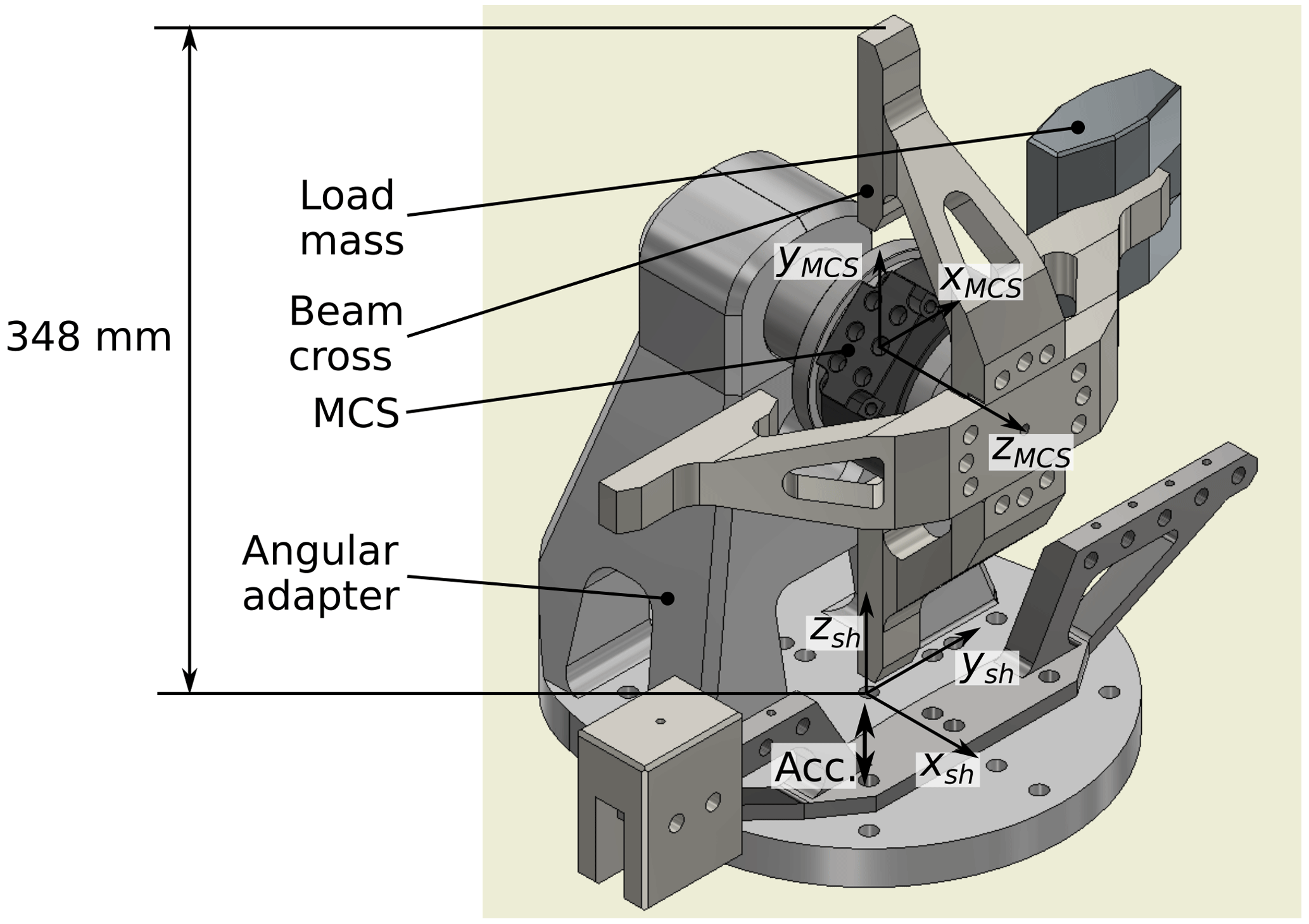
For the generation of moment components, a beam cross is used. The cross is designed in a way to move the centre of gravity of the moment generating mass components to the x–y plane of the sensor coordinate system. This results in a superposition of bending moments M_x or M_y with only one axial force F_z and the superposition of torque M_z with only one transverse force F_x or F_y. The distance between the load mass and the sensor can be changed to generate different amplitudes of the moment component. To reduce moment loads on the shaker bearing, a counter mass is attached to the base of the angular adapter. The beam cross set-up is shown in Fig. 3.

Figure 3 Beam cross for generation of moment components.

3.2 Three-dimensional acceleration reference

To evaluate whether signal outputs of inactive force or moment components of the sensor are a result of signal crosstalk from the active component or of bending or twisting moments, a complete three-dimensional movement of the set-up needs to be identified. The scanning vibrometer is capable of measuring the acceleration in the direction of the shaker axis at different points of the set-up. From the acceleration distribution, rocking modes around the x and y axes can be identified. Three-dimensional accelerometers can be added to specific points in the system to obtain three-dimensional acceleration information at that point. However, the mass of the accelerometer and its cable has an influence on the dynamic behaviour of the whole set-up.

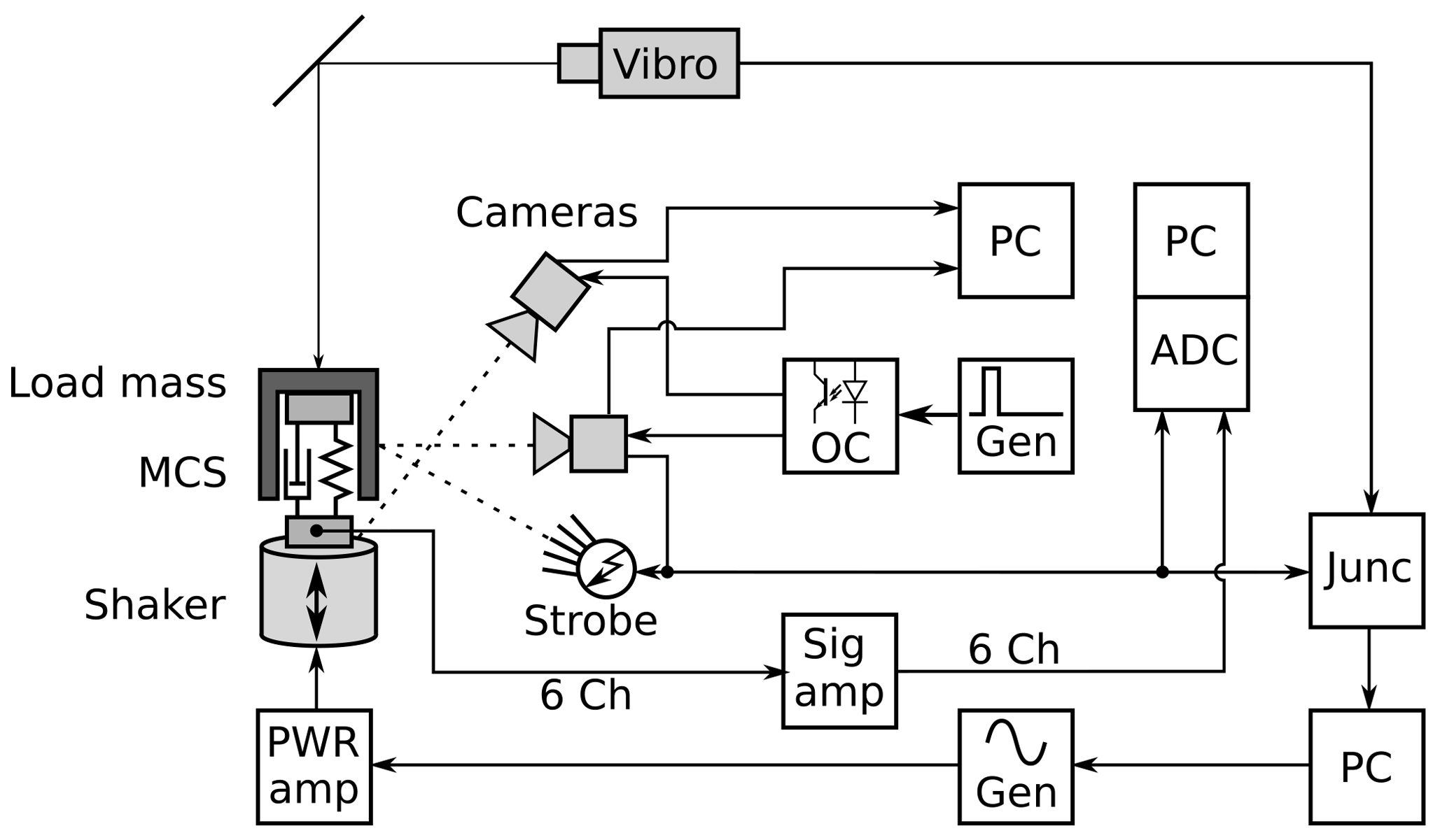
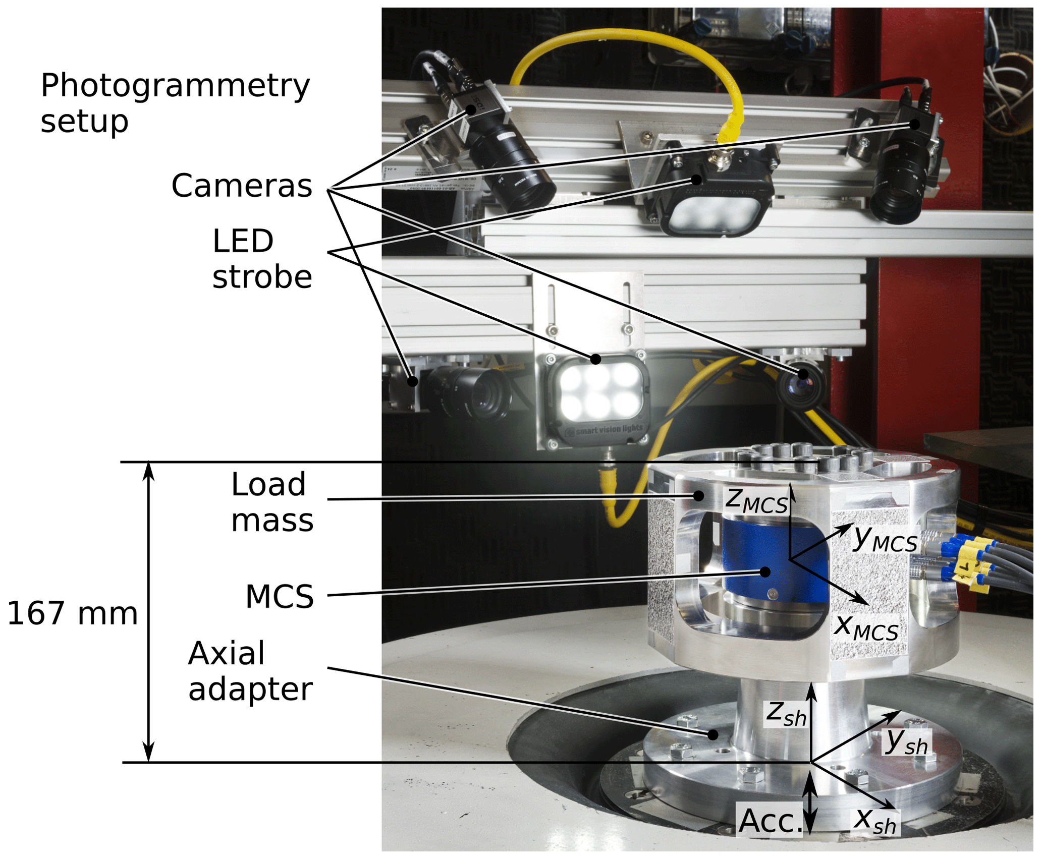
To extend the acceleration measurement provided by the laser vibrometer and the accelerometers, a photogrammetric measurement set-up is installed. It consists of two stereo camera systems: one camera system observing the load mass on top of the sensor, the other one directed at the surface of the shaker. All four cameras are triggered simultaneously using a signal generator. One master camera is used to trigger two LED strobe lights to illuminate the observed area. This trigger signal is recorded by the analogue to digital converter (ADC) in the junction box of the data acquisition PC of the scanning vibrometer for synchronization purposes. The trigger signal also serves as the time stamp of the image acquisition. The six force and moment signals of the sensor under test are amplified by a 6-channel bridge amplifier (Dewetron, 2012), digitized by a simultaneously sampling 16-channel ADC card (National Instruments, 2012) and saved on a separate data acquisition PC. The camera trigger signal is also recorded by this PC for synchronization. A block diagram of the extended shaker set-up is shown in Fig. 4. A photograph of the sensor with the attached load mass, the shaker and the stereo camera systems is shown in Fig. 5.

Figure 4 Block diagram of the photogrammetric set-up in the dynamic shaker system.

Figure 5 Photogrammetric set-up in the shaker environment.

Figure 6 Vibrometer and camera trigger signals.

Random greyscale patterns are attached to the surfaces observed by the cameras. The images of these patterns are analysed using digital image correlation (DIC) algorithms (Pan et al., 2009). In DIC, the camera images are split into small areas and the correlation between the areas in different camera images is calculated. In this way, one area of the observed surface can be identified in the images of both cameras and at different times. Each stereo set-up is able to calculate the position of multiple areas on the observed surface in space. Those three-dimensional points can be used to calculate a three-dimensional rigid body movement as well as a deformation of the load mass in the observed area.

The rotation and translation of the rigid body transformation are calculated using the singular value decomposition (SVD) method presented by Arun et al. (1987) (Eggert et al., 1997). From the resulting rotation matrix, the rotation angles are calculated in a fixed axis system. This assumption can be used as the rotations around any axis are expected to be very small and therefore do not influence each other.

Table 1 Fitted sine parameters.

The cameras used for DIC are industrial CMOS cameras with frame rates of up to 166 images per second for 8-bit greyscale images. At 12-bit colour depth, the frame rate is reduced to a maximum of 82 images per second. This frame rate is too low to satisfy the Nyquist–Shannon sampling theorem for frequencies higher than 40 Hz. However, using the additional knowledge of the excitation frequency of the shaker and the precise adjustment of the sampling rate of the cameras, both frequencies can be adjusted to achieve a beat frequency.

The known frequency distribution resulting from the vibrometer measurement is used to define a fitting function for the displacement of the load mass S(t):

$$\begin{array}{}\text{(5)}& S\left(t\right)=\sum _i\left({\widehat{s}}_i\cdot \sin \left(\mathrm{2}\cdot \mathit{\pi }\cdot f_{\mathrm{i}}\cdot t+{\mathit{\phi }}_i\right)\right)+o,\end{array}$$

with f_i as the identified frequencies of the frequency distribution, ${\widehat{s}}_i$ the amplitude, φ_i the phase shift of each frequency and o the offset of the mean. The parameters $\widehat{s}$, φ and o can be estimated by a least squares fitting algorithm. The resulting function S(t) represents the axial or angular displacement of the load mass over time.

3.3 Experimental analysis of the set-up

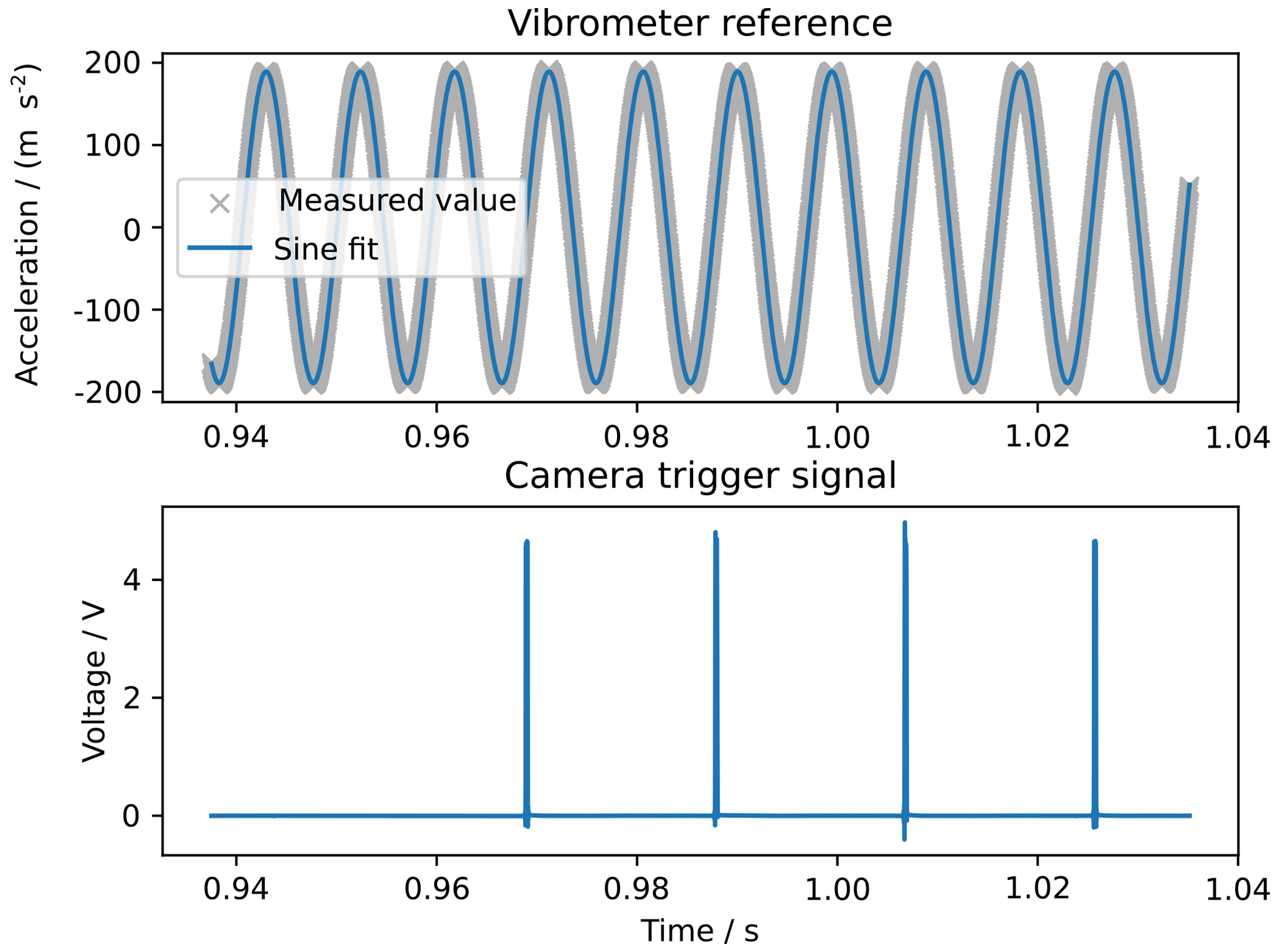
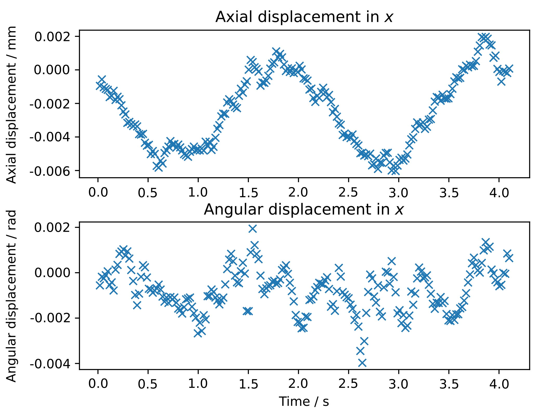
An experimental evaluation of the set-up described is performed using the axial force components. The excitation frequency is set to f_ex=106.25 Hz. The amplitude of the acceleration signal is 0.5 V. The laser vibrometer sampling frequency is 51.2 kHz and the cameras are triggered with 52.874 Hz. Figure 6 shows the acceleration signal recorded from the laser vibrometer, a fitted sine function and the camera trigger signal as a synchronization reference. The parameters of the sine fitting are listed in Table 1. The camera trigger is started manually after starting the vibrometer recording. The trigger signal at 0.97 s represents the first image acquired by the cameras.

The difference between the camera frequency and the excitation frequency results in a beat of 0.502 Hz. The first camera image is taken as a reference image against which all displacements are calculated. Each camera acquires 211 images, which results in 210 displacement measurements within 3.97 s.

For each displacement measurement, the rigid body transformation is calculated as described in Sect. 3.2. As a result, three axial translations and three rotation angles along the coordinate system of the camera set-up are obtained. For each displacement measurement, the mean of the exposure time, which is identified from the strobe trigger signal, is used as the time of acquisition. The data sets of acquisition time and axial and angular displacement are used to fit a sine function according to the excitation frequency of the shaker.

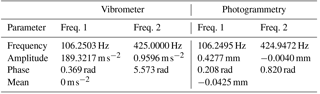
Sine fitting is performed using a nonlinear least squares fitting function, curve fit, of the Python scipy optimize package. Starting values for the fitting frequencies are taken from the frequency spectrum of the vibrometer reference. Figure 7 shows the frequencies of the fast Fourier transform (FFT) up to 1000 Hz.

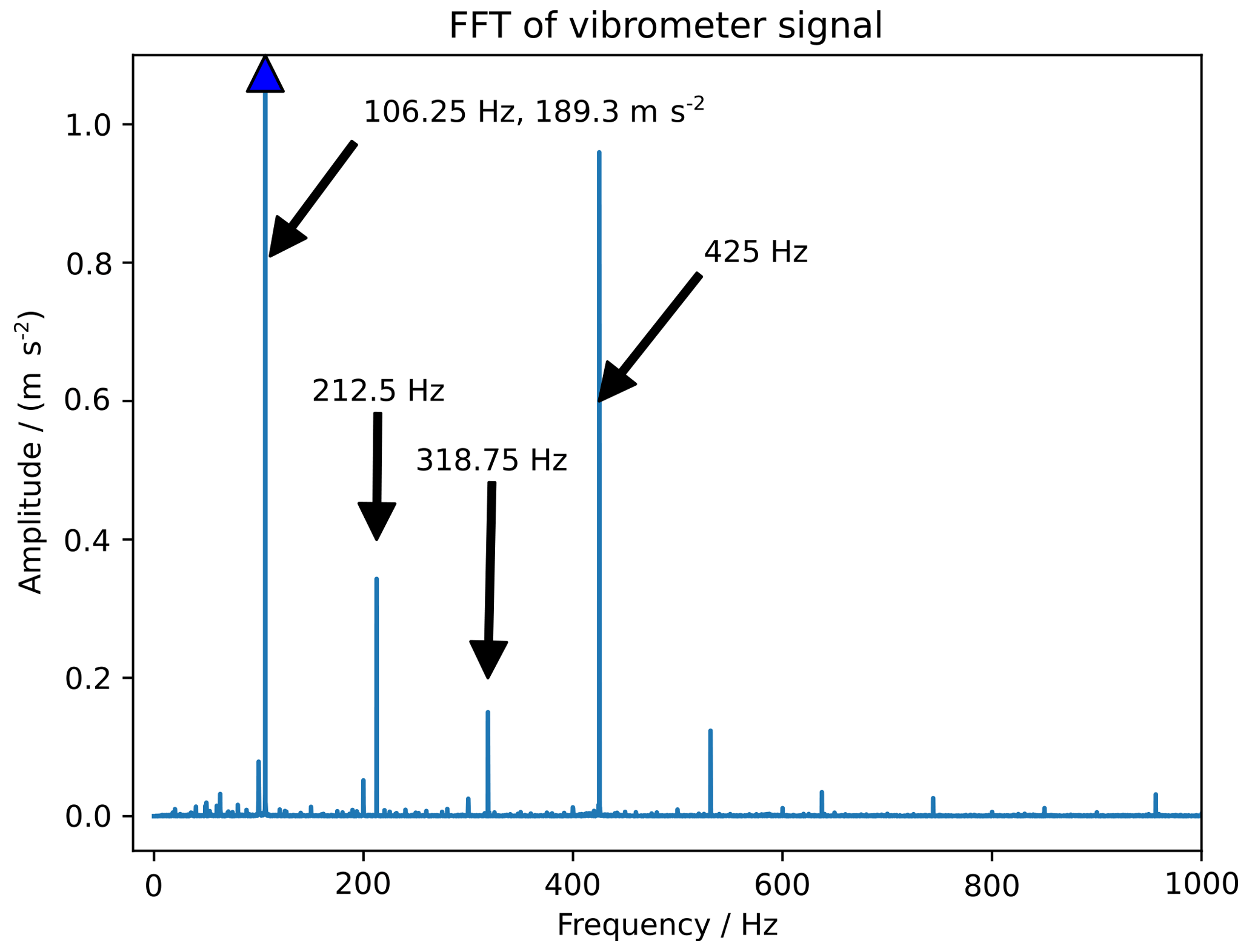
Figure 7 Frequency spectrum of the vibrometer signal. The y axis is scaled to make frequencies different than the excitation frequency visible. The amplitude of f_ex=106.25 Hz is 189.3 m s⁻².

Figure 8 Displacement in z from DIC and the fitted sine function.

The main contributions can be seen at the excitation frequency f_ex=106.25 Hz and its multiples 425, 212.5 and 318.75 Hz. The amplitude at the second frequency (425 Hz) reaches a value of 0.5 % of the amplitude of the excitation frequency.

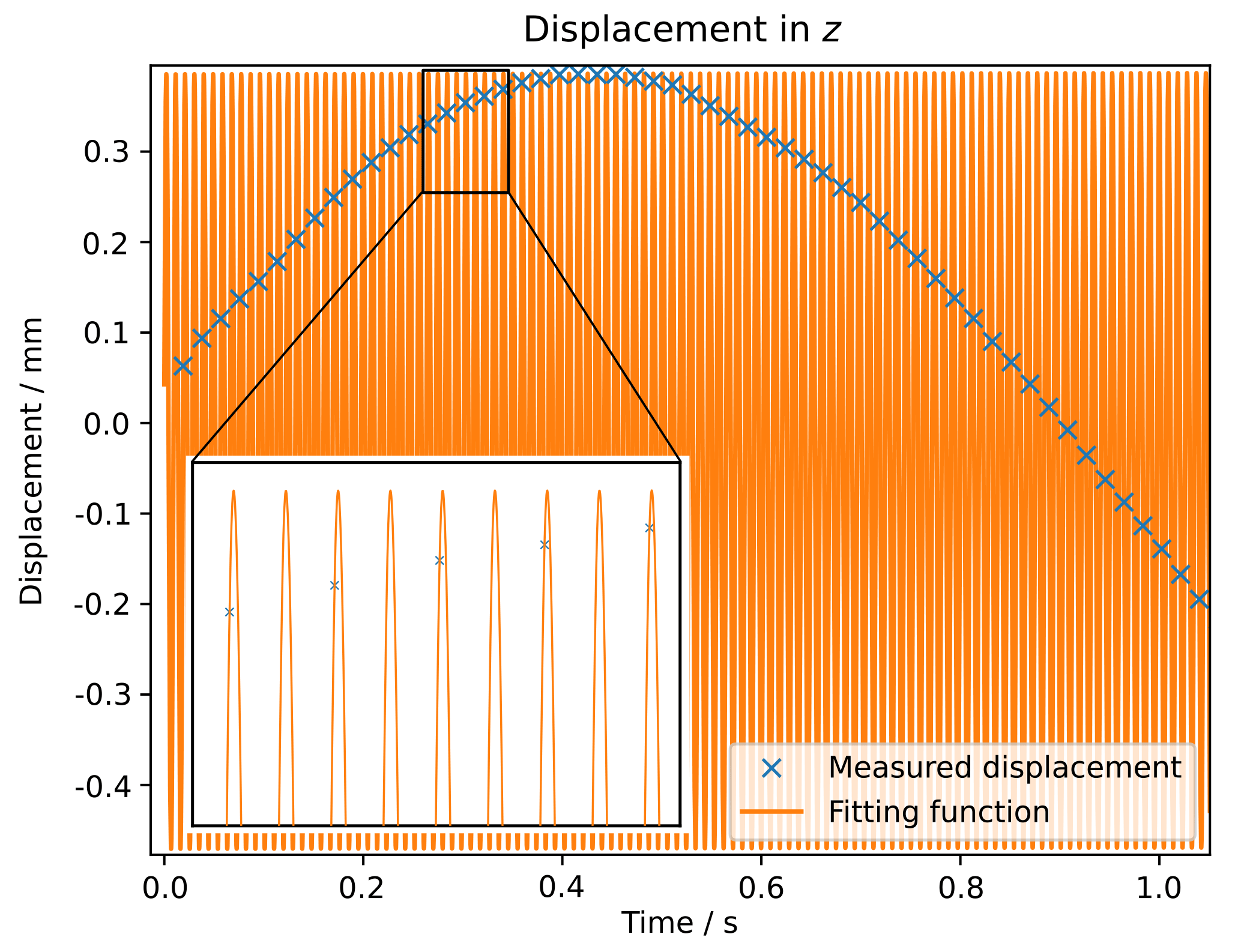
Sine fitting of only the excitation frequency f_ex=106.25 Hz results in a standard deviation of the difference between the fitting function and the measured displacements of 0.0036 mm. Using a fitting function of the two main frequencies 106.25 and 425 Hz reduces the standard deviation of the residuum to 0.0023 mm. Additional fitting frequencies show no further improvement of the results. The displacement in z, measured with the photogrammetry set-up and the fitted sine function, is shown in Fig. 8. Figure 9 shows the axial and angular displacement along the x axis. The resulting parameters from the sine fitting are listed in Table 1.

Figure 9 Axial and angular displacement in x.

To calculate the resulting force and moment components on the sensor, the axial and angular acceleration of the load mass is needed. Both values can be calculated from the fitting function of the displacement as the second derivative with respect to time. For a sine function, the second derivative can easily be calculated by multiplying the function by the negative square of the angular frequency ${\mathit{\omega }}_i=\mathrm{2}\cdot \mathit{\pi }\cdot f_{\mathrm{i}}$. The acceleration of the fitting function of Eq. (5) results in

$$\begin{array}{}\text{(6)}& \ddot{S}\left(t\right)=\sum _i\left(-{\widehat{s}}_i\cdot {\mathit{\omega }}_i^{\mathrm{2}}\cdot \sin \left({\mathit{\omega }}_i\cdot t+{\mathit{\phi }}_i\right)\right).\end{array}$$

From the values of the fitting function listed in Table 1, the amplitude of the acceleration ${\widehat{a}}_i=-{\mathit{\omega }}^{\mathrm{2}}\cdot {\widehat{s}}_i$ from the photogrammetric measurement is calculated to be ${\widehat{a}}_{\mathrm{1}}=-\mathrm{190.6131}$ m s⁻² and ${\widehat{a}}_{\mathrm{2}}=\mathrm{28.5161}$ m s⁻². While the acceleration at the excitation frequency shows a small deviation of 0.68 % to the reference value of the vibrometer, the acceleration at 425 Hz differs significantly. According to the reference acceleration, the amplitude of the second frequency has a minor influence on the overall acceleration and will be neglected in the subsequent analysis. It must however be included in the pending uncertainty budget.

4 Dynamic model of multi-component sensors

For uniaxial force sensors, a dual-mass oscillator as shown in Fig. 1 can be used as an acceptable description of the dynamic behaviour (Kumme, 1996; Schlegel et al., 2012). MCSs show a more complex structure which results in a more complex physical model. To reduce the complexity of the model, the observed six-component MCS is split into two independent models, one for the three force components, one for the moment components.

4.1 Dynamic MC force model

The dynamic model for a three-component force sensor is based on a superposition of three orthogonally aligned spring-damper systems connected to two masses m₁ and m₂. A simplified illustration of a two-dimensional case of this model is shown in Fig. 10. Mutual influences between the spring-damper systems are neglected. To describe this model, eight different parameters are needed: three spring constants k_x, k_y, k_z, three damping parameters b_x, b_y, b_z and the two masses m₁ and m₂. The masses are assumed to be equal for excitation in the x, y and z directions.

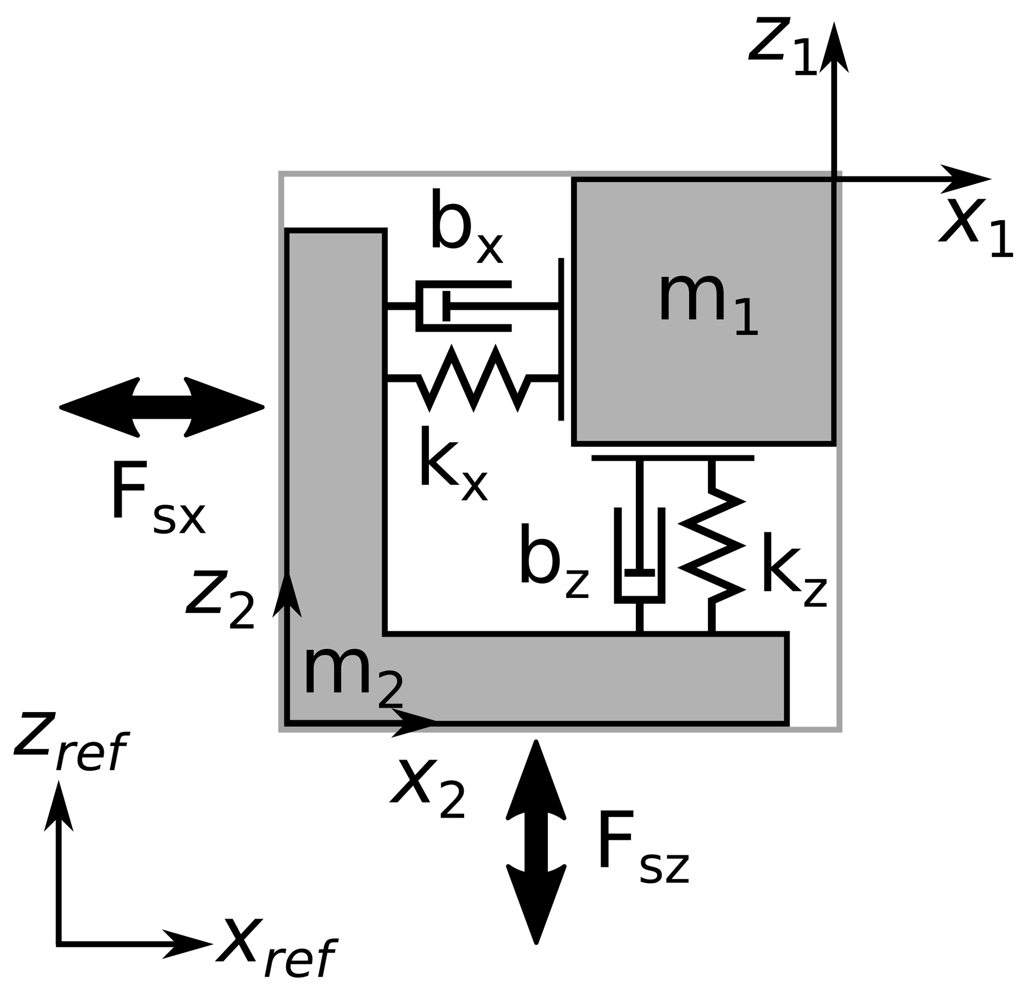
Figure 10 Two-dimensional representation of the dual-mass oscillator for multi-component force sensors.

4.2 Dynamic MC moment model

A dynamic model for a three-component moment sensor is more complex than the model for a three-component force sensor. Basically, the model from Fig. 10 can be adapted by changing the springs and dampers of the model from linear to rotational ones. The exchange of the masses is more difficult, as the mass moment of inertia is needed for dynamic moment measurements. This parameter depends on a rotational axis and therefore it cannot be assumed to be equal for the different excitation directions.

5 Parameter identification

5.1 Determination of the internal mass

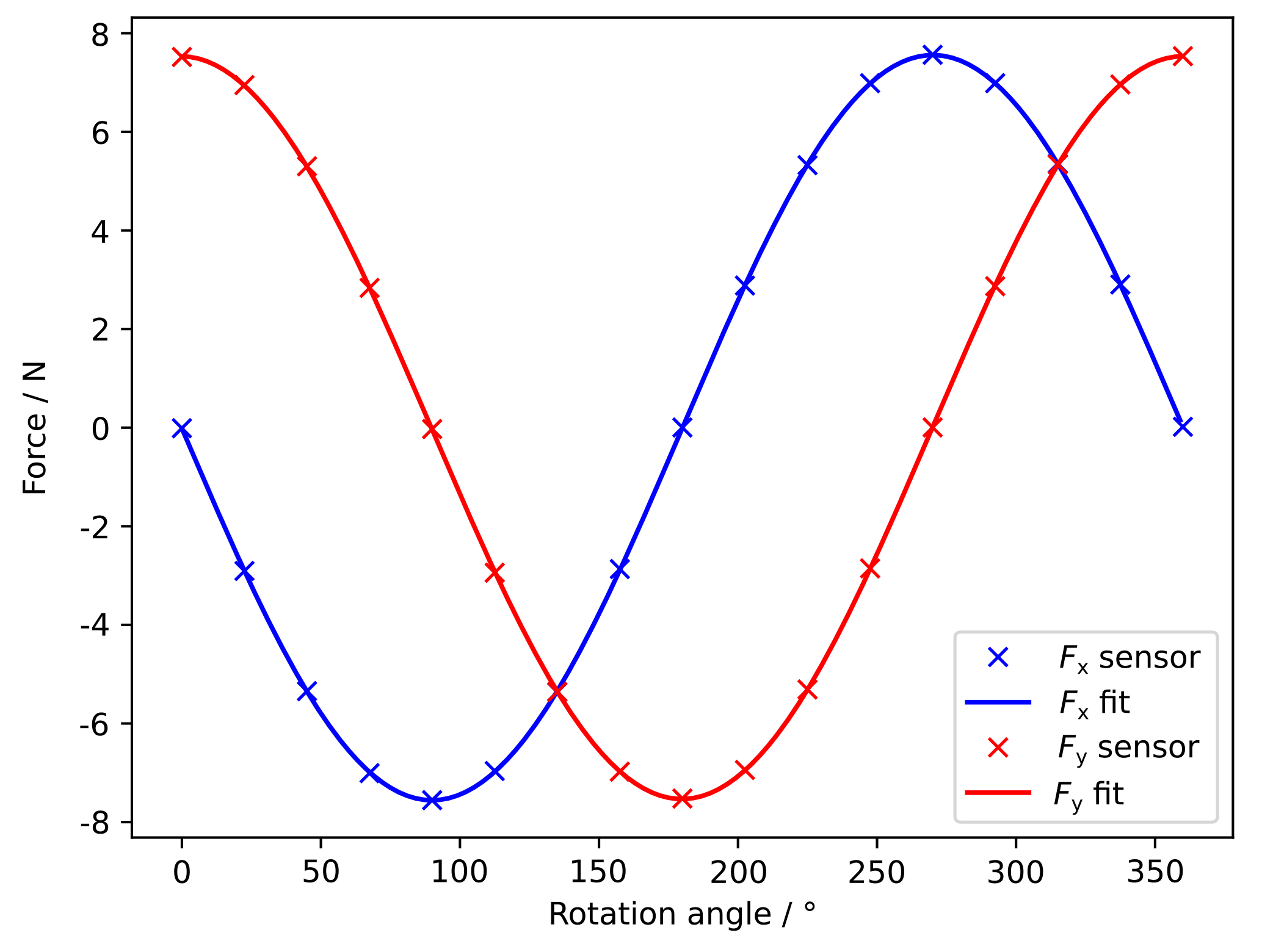
To determine the internal mass m₁ of the sensor, the sensor is mounted onto an indexing head with a horizontal rotation axis. The z axis of the sensor is aligned with the rotation axis of the indexing head. Sensor readings are recorded without an attached load mass. The sensor is rotated in steps of 22.5^∘. The sensor readings are transformed into force and moment values using the calibration matrix provided by the sensor manufacturer. A sine function is fitted to the force values for F_x and F_y. The amplitude of the sine function represents the maximum force on each channel resulting from the internal mass of the sensor. The mass itself is calculated from the amplitude, divided by the local acceleration of gravity g_loc:

$$\begin{array}{}\text{(7)}& m_{\mathrm{1}}={\displaystyle \frac{F_{\max }}{g_{\mathrm{loc}}}}.\end{array}$$

Force readings and the sine fitting for F_x and F_y are shown in Fig. 11. The resulting amplitude of the sine function is 7.558 N for F_x and 7.532 N for F_y, resulting in internal masses of m_1x=0.770 kg and m_1y=0.768 kg.

Figure 11 Force readings and sine fitting for F_x and F_y.

The described experiment is repeated with the load mass shown in Fig. 2 attached to the sensor. Including the attached load mass, the amplitude of the sine function is 75.877 N for F_x and 75.736 N for F_y. The mass of the attached load mass is calculated according to Eq. (7) to m_Lx=6.962 and m_Ly=6.951 kg, which differ by 0.028 % and −0.139 % respectively from the weighted mass m_L=6.9605 kg.

5.2 Determination of the spring constant and damping coefficient

The spring constant is calculated according to the method presented by Schlegel et al. (2012) from the transfer function H(f) as the ratio of the acceleration on the load mass a_t and the acceleration of the shaker surface a_b:

$$\begin{array}{}\text{(8)}& H\left(f\right)={\displaystyle \frac{a_{\mathrm{t}}}{a_b}}.\end{array}$$

The frequency of the maximum of the transfer function represents the resonance frequency f₀, from which the spring constant can be calculated:

$$\begin{array}{}\text{(9)}& f_{\mathrm{0}}={\displaystyle \frac{\mathrm{1}}{\mathrm{2}\mathit{\pi }}}\sqrt{{\displaystyle \frac{k}{m}}}.\end{array}$$

The transfer function H(f) for F_z, resulting from a periodic chirp excitation with two different load masses m₁=4.236 kg and m₂=8.798 kg, is shown in Fig. 12. Resonance frequencies are identified at $f_{\mathrm{0},\mathrm{1}}=\mathrm{1477.35}$ Hz and $f_{\mathrm{0},\mathrm{2}}=\mathrm{1092.97}$ Hz. With the additional internal mass m_i=0.769 kg, the spring constant according to Eq. (9) is calculated to be $k_{\mathrm{1}}=\mathrm{4.313}\times {\mathrm{10}}^{\mathrm{8}}$ N m⁻¹ and $k_{\mathrm{2}}=\mathrm{4.512}\times {\mathrm{10}}^{\mathrm{8}}$ N m⁻¹.

Figure 12 Amplitude and phase of the transfer function H(f) for excitation in F_z.

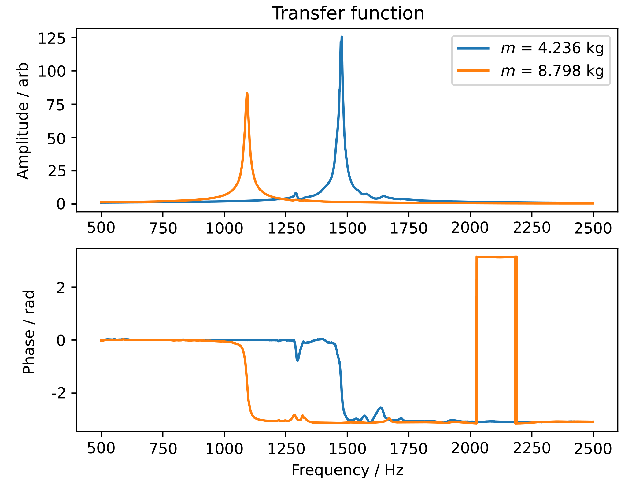
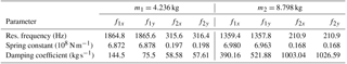
Figure 13 shows the transfer function H(f) for excitation in F_x and F_y. Because of the horizontal installation of the sensor (Fig. 2), the transfer function is calculated as the ratio of the acceleration of the load mass and the acceleration of the mounting adapter connected to the sensor. The figure shows two resonance peaks for each load mass, which can be explained by the mounting set-up. The connection between the horizontal mounting adapter connected to the sensor and the angular adapter introduces a second spring-damper system into the model. It can be seen that the resonance frequencies are identical for excitation in F_x and F_y, while the amplitudes of the resonance peaks differ for the higher resonance frequencies. The identified resonance frequencies and the resulting spring coefficients are listed in Table 2.

Figure 13 Amplitude of the transfer function H(f) for excitation in F_x and F_y.

Table 2 Resonance frequencies, spring constants and damping coefficients for force excitation in x and y.

In Schlegel et al. (2012), the damping coefficient of the spring-damper model is calculated using the ratio of the resonance frequency and the width of the resonance peak of the transfer function at half the amplitude:

$$\begin{array}{}\text{(10)}& {\displaystyle \frac{f_{\mathrm{0}}}{\mathrm{\Delta }{f}_{\mathrm{1}/\mathrm{2}}}}\approx {\displaystyle \frac{\mathrm{1}}{b}}\sqrt{k\cdot m}.\end{array}$$

For the given transfer function in Fig. 12, the damping coefficients are calculated to be b₁=699.18 kg s⁻¹ and b₂=1566.01 kg s⁻¹. The damping coefficients for excitation in x and y are listed in Table 2.

5.3 Determination of the dynamic sensitivity and phase shift

To calculate the dynamic sensitivity of the sensor, sinusoidal excitations at different frequencies are used. Measurements are performed at 12 different frequencies from 53.7 to 1020.3 Hz. The sensitivity S is calculated from the ratio of the amplitude of the sensor signal $\widehat{s}$, the top mass m_t and the amplitude of the top mass acceleration ${\widehat{a}}_{\mathrm{t}}$:

$$\begin{array}{}\text{(11)}& S={\displaystyle \frac{\widehat{s}}{{\widehat{a}}_{\mathrm{t}}\cdot m}}.\end{array}$$

The acceleration ${\widehat{a}}_{\mathrm{t}}$ is measured at eight different positions on the top mass using the laser vibrometer.

The phase shift between the acceleration of the top mass a_t and the sensor signal s is calculated from the phase of the sine fitting functions of the sensor and the vibrometer signal. The synchronization between the signal sources is performed using the camera trigger signal as described in Sect. 3.2.

Figure 14 shows the mean value of the dynamic sensitivity and the phase shift over the eight acceleration measurements and the resulting standard deviation. The static sensitivity from the sensor calibration data is given as a reference. A rocking mode occurs at a frequency of 375.9 Hz, which leads to higher deviations for the acceleration measurements in the outer areas of the load mass. The rocking motion can also be seen in the higher standard deviation of the phase shift values. Up to the excitation frequency of 1000 Hz, the sensitivity drops to 95.3 % of the static value. The phase shift drops to −0.25 rad at 800 Hz. For higher frequencies up to 1000 Hz, the phase shift does not change significantly.

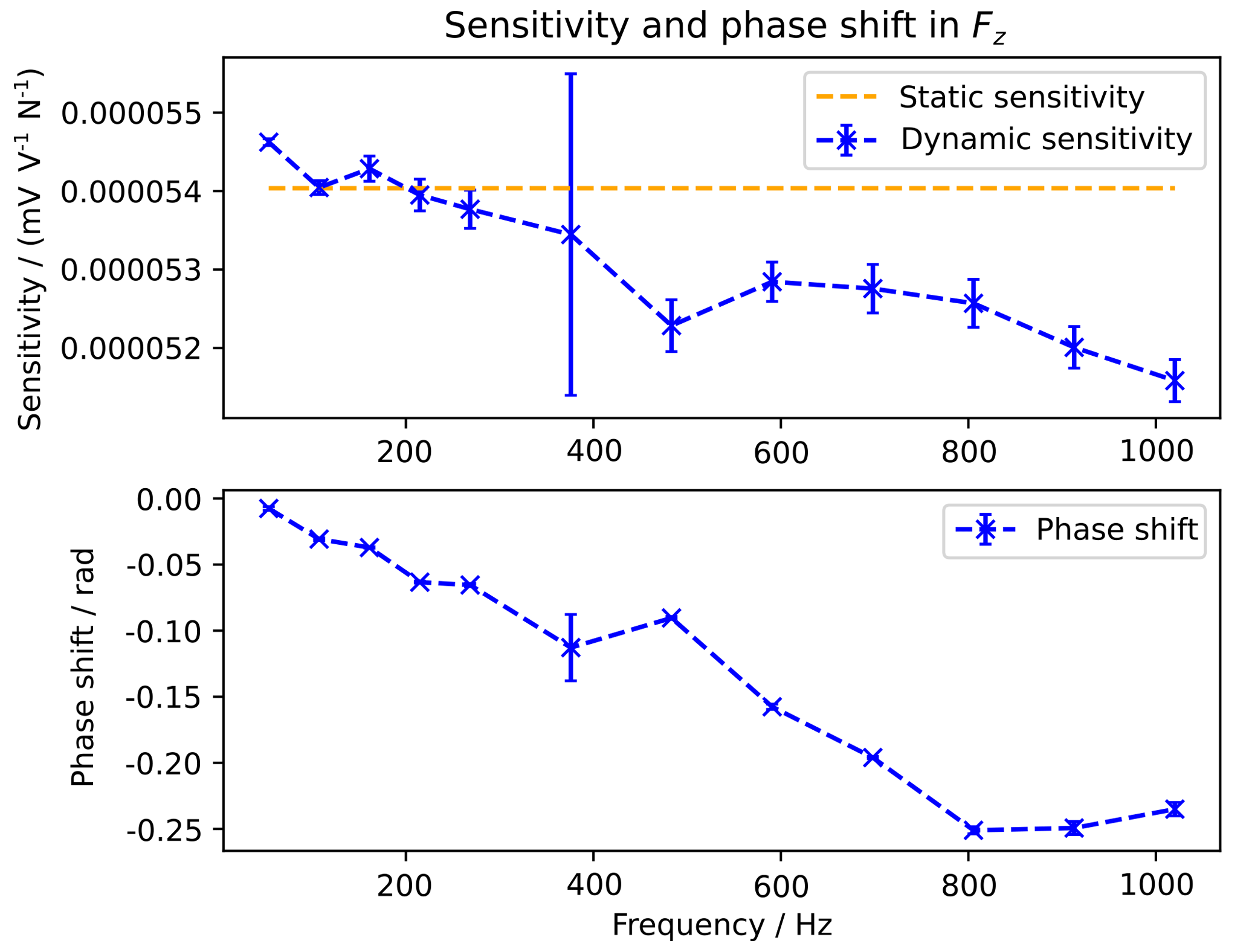
Figure 14 Sensitivity of F_z and phase shift between top mass acceleration and sensor signal. Error bars represent the standard deviation for the acceleration at eight different positions on the top mass.

6 Conclusions

An extended set-up for the dynamic calibration of multi-component sensors for force and moment measurement has been described. It is based on the periodic acceleration of a sensor and an attached load mass on an electrodynamic shaker. In comparison to earlier works, the design of the load mass and adapting elements was focused on activating single force and moment components where possible. Force components can be activated using a load mass with its centre of gravity in the origin of the sensor coordinate system. For the moment components, a beam cross with a movable load mass was designed.

To identify the movement of the load mass with 6 degrees of freedom, a photogrammetric set-up was installed in the existing laboratory set-up. Two stereo camera systems observe the load mass and the shaker surface. From the displacement of the observed surfaces and the time stamp of the camera images, accelerations can be calculated. With the additional information of the excitation frequency and reference measurements using a laser interferometer, the displacement of the set-up can be calculated even with camera frame rates lower than the excitation frequency. From an experimental evaluation, a deviation of 0.68 % of the acceleration was achieved for an excitation frequency of f_ex=106.25 Hz.

The dynamic parameters of the sensor are identified based on a three-dimensional mass-spring-damper system. The internal mass of the sensor was calculated in a static manner from measurements at different rotation angles around the z axis. The resulting internal masses of x=0.77 and y=0.768 kg differ by 0.3 %. The spring constant was calculated from a transfer function as the ratio of the top mass acceleration and the acceleration of the shaker surface. For two different load masses, the resulting spring constant differs by 4.4 % for F_z. The spring constant for excitation in the x and y directions shows small deviations of less than 0.5 % for the different orientations with the same load mass, while the difference at different load masses for the same orientation rises to up to 15 %. It has to be pointed out that the adapting elements for excitation in the x and y directions are still subject to optimization. At frequencies from 350 to 500 Hz, pitching motions occur which show an influence on the measurements.

The dynamic sensitivity of the sensor was analysed for the F_z component. In this set-up, a rocking motion is visible at 375.9 Hz, which increases the standard deviation of the measured accelerations on the top mass. Up to a frequency of 1000 Hz, the dynamic sensitivity drops to 95.3 % of the static value. The phase shift between the sensor signal and the top mass acceleration drops to −0.25 rad at frequencies of 800 Hz.

As a next step, the analysis performed will be extended to the moment excitation. The previously described beam cross and moment excitation mass are currently being manufactured. Further optimization of the horizontal set-up to reduce pitching motions is suggested to reduce signal crosstalk. Alternatively, a three-dimensional shaker set-up can be used in combination with the adapting element for F_z excitation. Finally, the measurement uncertainty for the different set-ups will be analysed.