Granular metal–carbon nanocomposites as piezoresistive sensor films – Part 2: Modeling longitudinal and transverse strain sensitivity

Granular and columnar nickel–carbon composites may exhibit large strain sensitivity, which makes them an interesting sensor material. Based on experimental results and morphological characterization of the material, we develop a model of the electron transport in the film and use it to explain its piezoresistive effect. First we describe a model for the electron transport from particle to particle. The model is then applied in Monte Carlo simulations of the resistance and strain properties of the disordered films that give a first explanation of film properties. The simulations give insights into the origin of the transverse sensitivity and show the influence of various parameters such as particle separation and geometric disorder. An important influence towards larger strain sensitivity is local strain enhancement due to different elastic moduli of metal particles and carbon matrix.

1 Introduction

In our associated paper, part 1 (Schultes et al., 2018), experimental results and film morphology of metal–carbon films were presented. We continue by presenting a model and simulation results for nickel–carbon (Ni:a–C:H) thin films. The properties of such films are discussed, especially the enhanced longitudinal and transverse gauge factors. The model links film morphology, electron transport, and mechanical strain. Results of numerical Monte Carlo simulations of the gauge factors of the films are presented to show different parameter influences.

Nickel–carbon films offer high stability and large gauge factors (k) with a tunable temperature coefficient of resistivity (TCR). A gauge factor maximum was found for metal concentrations of 55±5 at. %. The highest gauge factors were about 30. Not only did the films have large gauge factors when strained longitudinally to the resistance path but also with transverse strain as well. The transverse sensitivity is about 0.5 of the longitudinal one.

The morphology was analyzed by means of transmission electron microscopy (TEM). The films consist of columnar nickel particles encapsulated in several atomic layers of graphite-like carbon. A schematic diagram of the columnar structure is shown in Fig. 1.

To understand the strain sensing properties of the granular film, we first consider the charge-transport mechanism. Due to the heterogeneous conductivity, i.e., highly conductive metal particles and relatively poorly conductive barriers of carbon, electrons will tunnel between metal particles. The nature of the piezoresistive effect in granular metals is the following: strain affects electron tunneling distances, leading to changes in conductivity and thus results in strain sensitivity (Huth, 2010).

This effect occurs in several composite materials with local regions of different conductivity, e.g., in diamond-like carbon (Tibrewala et al., 2007b; conductive regions of sp² bonds surrounded by insulating regions of sp³ bonds) and in metal-composite films, which exhibit enhanced gauge factors when separated metal particles are embedded in an insulating matrix material, i.e., granular metals (Hill et al., 1982; Schwalb et al., 2010).

Although all of the materials mentioned above have been investigated in terms of their strain sensitivity in the longitudinal direction, only in some cases has this been extended to the transverse sensitivity (Schubert et al., 1987; Tibrewala et al., 2007a; Jiang et al., 2015). We present an analysis for the longitudinal and transverse gauge factors for columnar nickel–carbon films.

Figure 1 Simplified representation of a columnar nickel–carbon film on a substrate.

2 Modeling

We set out to find a model for the thin film that allows us to explain the enhanced longitudinal and transverse gauge factors and some parameters they depend on. First, mechanisms of electron transport are investigated. Then, we propose a model for the geometric structure of the material. For this, we represent the columnar geometry (Fig. 1) as an essentially two-dimensional structure, i.e., an arrangement of circles. Finally, electron transport and geometry are combined to perform calculations regarding the electro-mechanical properties of the material.

2.1 Conductivity in granular metal films

Literature on granular metals describes their electrical conductivity for several domains depending on temperature and electrical coupling (field strength) (Beloborodov et al., 2007; Huth, 2010). For room temperature and above with relatively low voltages (a voltage ΔV between particles so that $e\cdot \mathrm{\Delta }V\ll k_B\cdot T$), conductivity is expected to follow a thermally activated electron tunneling behavior of Arrhenius form Huth (2010)

$$\begin{array}{}\text{(1)}& {\displaystyle }{\displaystyle }\mathit{\sigma }\left(T\right)={\mathit{\sigma }}_{\mathrm{0}}\cdot e^{-\frac{{\mathrm{\Delta }}_{\text{M}}}{k_{B}T}},\end{array}$$

with the Mott gap ${\mathrm{\Delta }}_{\text{M}}=f(s,E_{\mathrm{C}})$ that depends on particle separation s and Coulomb energy $E_{\mathrm{C}}=e^{\mathrm{2}}/(\mathrm{2}\cdot C)$ (fundamental charge e, capacitance C). The Coulomb energy is the charging energy required to remove an electron from one metallic particle and transfer it to another. Spherical nanoparticles of a few nanometers in size have a small capacitance and an E_C comparable to the thermal energy k_BT at temperatures of 300 K, thus it has to be considered. The large columnar particles in the Ni:a–C:H films presented here have a much greater capacitance, so the influence of E_C can be neglected.

For a simplified approach at a given temperature, the conductive mechanism can be described by the Arrhenius-form tunneling conductivity (Canali et al., 1980; Jiang et al., 2015). The relative change of resistance, ΔR∕R₀, depends on the change in particle separation, Δs, in the form of

$$\begin{array}{}\text{(2)}& {\displaystyle }{\displaystyle \frac{\mathrm{\Delta }R}{R_{\mathrm{0}}}}=e^{\mathit{\beta }\cdot \mathrm{\Delta }s}-\mathrm{1},\end{array}$$

with the attenuation length β.

For a simple model approach, we consider a granular metal–matrix system with a matrix material that has an isotropic resistivity. The metallic intra-particle resistance is lower than the matrix resistance by several orders of magnitude, as evidenced by the much higher resistivity of metal–carbon samples compared to purely metallic thin films. Thus, the conductance across the sample can be viewed as electron transport from one metal particle to the next through an interjacent area of carbon.

Percolated films with a large metal content will behave like metallic films. They have gauge factors of k≈2 due to the geometric effect of strain. Our work focuses on the piezoresistive effect in the films, therefore the case of metallic films is not covered in the model.

The effective conductance between two neighboring particles is the sum of the conductance through the matrix material and the electron tunneling conductance between the particles. Both conductivities depend on the particle separation distance s. The matrix material conductivity is linear in s, the tunneling conductance is exponential in s.

Figure 2 Resistor model from one particle to the next.

Figure 3 Hexagonal cluster networks in different orientations φ.

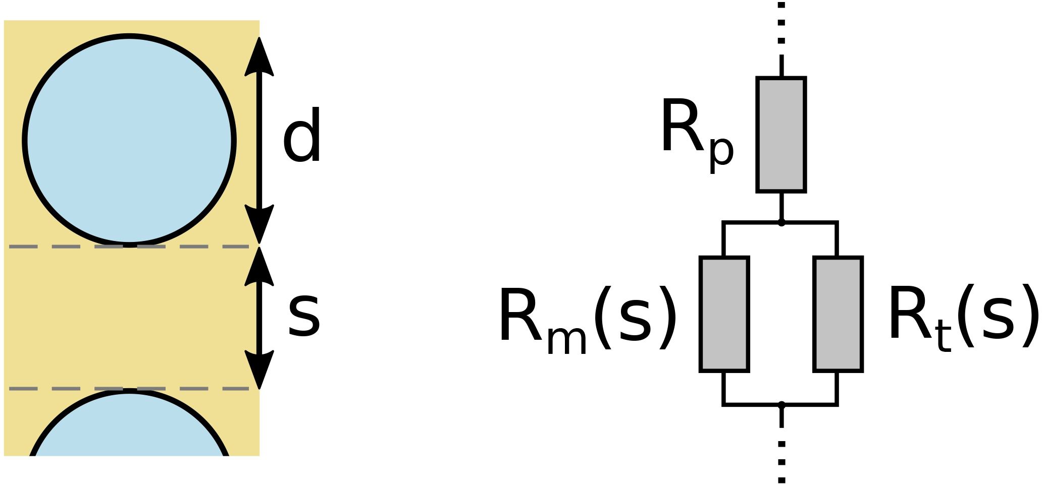
In terms of an electrical resistance network, the tunneling resistance R_t is in parallel with the matrix material resistance R_m, with both of these in series with the resistance R_p of the metal particle itself, as schematically shown in Fig. 2. These combined resistances form the basic element of the resistance network, the particle-to-particle resistance

$$\begin{array}{}\text{(3)}& {\displaystyle }{\displaystyle }R={\displaystyle \frac{R_{\mathrm{t}}\cdot R_{\mathrm{m}}}{R_{\mathrm{t}}+R_{\mathrm{m}}}}+R_{\mathrm{p}},\end{array}$$

which includes the linear matrix material resistance

$$\begin{array}{}\text{(4)}& {\displaystyle }{\displaystyle }{R}_{\mathrm{m}}\left(s\right)=a\cdot s,\end{array}$$

with the coefficient a of the linear matrix material resistance, and the exponential tunneling resistance

$$\begin{array}{}\text{(5)}& {\displaystyle }{\displaystyle }{R}_{\mathrm{t}}\left(s\right)=b\cdot e^{c\cdot s},\end{array}$$

with the pre-exponential coefficient b and the attenuation length c of the tunneling resistance.

The particle resistance R_p is approximated by considering a path of metallic conduction through the diameter of a columnar particle. With the two parallel mechanisms for inter-particle resistance and a value for intra-particle resistance, we can describe the effective resistance between two particles with the resistance law

$$\begin{array}{}\text{(6)}& {\displaystyle }{\displaystyle }R\left(s\right)={\displaystyle \frac{s\cdot a\cdot b\cdot e^{c\cdot s}}{a\cdot s+b\cdot e^{c\cdot s}}}+R_{\mathrm{p}}.\end{array}$$

The resistance calculation accounts for the strain influence on the particle separation. Our model does not cover the gauge factor of a significantly percolated film with its metallic conduction – as the resistance will be constant in this case and k_L and k_T will approach zero.

Finally, the gauge factor can be derived from the resistance law R(s) of Eq. (6). Its general equation is

$$\begin{array}{}\text{(7)}& {\displaystyle }{\displaystyle }k\left(s\right)={\displaystyle \frac{\mathrm{\Delta }R}{R\mathit{\epsilon }}}={\displaystyle \frac{\mathrm{\Delta }R}{\mathrm{\Delta }s}}{\displaystyle \frac{s}{R}}.\end{array}$$

By considering the relation

$$\begin{array}{}\text{(8)}& {\displaystyle }{\displaystyle \frac{\mathrm{\Delta }R}{\mathrm{\Delta }s}}{|}_{\mathrm{\Delta }s\to \mathrm{0}}={\displaystyle \frac{\mathrm{d}R}{\mathrm{d}s}}={\displaystyle \frac{a\cdot b\cdot e^{c\cdot s}\left(a\cdot c\cdot s^{\mathrm{2}}+b\cdot e^{c\cdot s}\right)}{{\left(a\cdot s+b\cdot e^{c\cdot s}\right)}^{\mathrm{2}}}},\end{array}$$

we find that

$$\begin{array}{}\text{(9)}& {\displaystyle }{\displaystyle }k\left(s\right)={\displaystyle \frac{s\cdot a\cdot b\cdot e^{c\cdot s}\left(a\cdot c\cdot s^{\mathrm{2}}+b\cdot e^{c\cdot s}\right)}{{\left(a\cdot s+b\cdot e^{c\cdot s}\right)}^{\mathrm{2}}\left(\frac{s\cdot a\cdot b\cdot e^{c\cdot s}}{a\cdot s+b\cdot e^{c\cdot s}}+R_{\mathrm{p}}\right)}},\end{array}$$

which is the gauge factor of a single particle-to-particle element for small strain of a given separation distance s. The resistance law (Eq. 6) and gauge factor (Eq. 9) are plotted vs. s in Fig. 5.

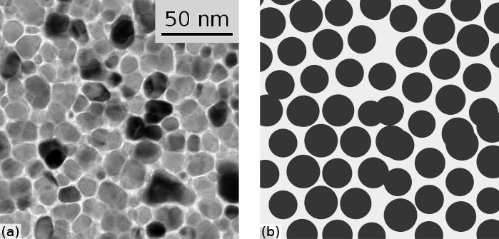
Figure 4 TEM image and model representation of the disordered film. (a) Top-view TEM image, (b) geometric model with four subsections of different random orientation (in each quarter of the image) and normally distributed diameters.

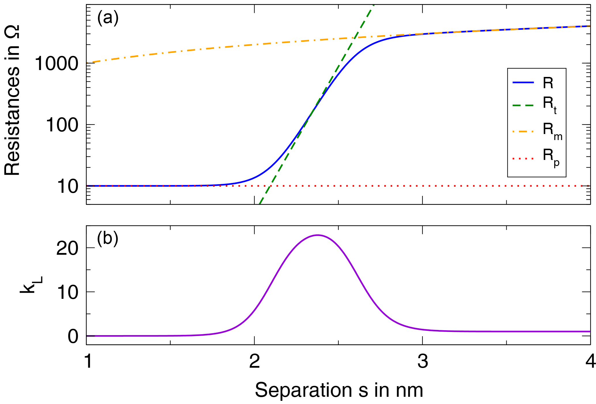
Figure 5 Analytical results for a single particle-to-particle junction. (a) Total resistance R and its individual components: exponential tunneling resistance R_t, linear matrix material resistance R_m, and the small and constant metal particle resistance R_p. (b) Resulting longitudinal gauge factor k_L.

2.2 Resistance network as a global model

To consider not only the electrical properties described previously but also the heterogeneous mechanical properties of the metal–carbon composite material and the geometric disorder of particles in the film, a global model built from a network of particles will be derived. We assume that a large number of columnar metal particles with some given diameter is arranged in a certain pattern (see Fig. 1). Each particle has a fixed number of next neighbors and corresponding particle-to-particle resistances. In full, this constitutes a large resistor network in which each particle is a node. To calculate the electrical material properties, the effective resistance through this particle array is calculated.

Using the TEM images we can find a mean separating distance s between columns and observe some slight deviations from it. The columns themselves vary in diameter; their number of next neighbors is typically 6±1. For our model, we choose a geometrically similar representation for this structure: a hexagonal grid of circular columns whose diameters follow a normal distribution around a certain mean value. This leads to a system equivalent to the one observed, where columns have six neighbors surrounding them, with slightly varying separating distances. This structure is modeled as a geometrically two-dimensional system.

The direction of the particle-to-next-neighbor paths does not follow any particular order and is assumed to be equally distributed for all directions for any sufficiently large area of the thin film.

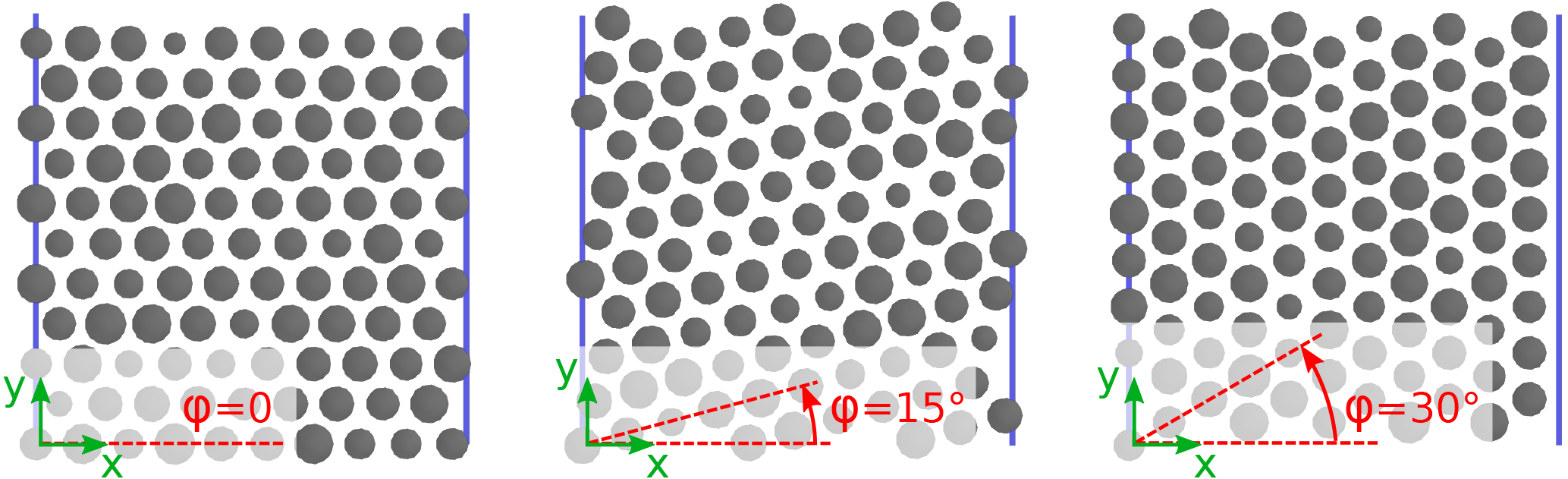
A regular hexagonal grid includes preferred directions for electron transport, which might exist locally in the actual thin film, but are not found on a large scale. To account for this, we introduce the angle φ by which the grid can be rotated (see Fig. 3). For the simulation, we solve the system for various angles in the interval $\mathit{\phi }\in [\mathrm{0},\mathrm{30}{}^{\circ }]$ to numerically integrate the resistances and gauge factors over all possible orientations. This model corresponds to a thin film made up of local areas of different orientations as shown in Fig. 4.

The circular column model is an approximation of the real material. If the model geometry is chosen with particle separation distances equal to the actual material, larger void areas appear compared to the slightly irregularly-formed columns of the real sample. This does not affect the simulation results as far as gauge factors are concerned, but introduces an offset of the metal content: for the same separation distances, the model film will have a lower metal content than the real material.

When a strain is applied to the network, a softer matrix material will result in locally enhanced strain (Grimaldi et al., 2001). To account for this effect, the calculation of local strain considers the elastic moduli E_p and E_m of the metal particles and the matrix material, respectively.

3 Numerical simulation

We now have a model that contains a representation of the film's geometrical structure, its mechanical response to strain, and the particle-to-particle electrical conduction. It allows us to find results for the longitudinal and transverse gauge factor for columnar metal-in-insulator films for different particle diameters and separation distances.

The numerical model is set up according to the following steps:

1. Randomly generate normal (or log-normal) distribution of column diameters d_i for a given mean diameter d_mean and a standard deviation (SD) of σ_d.

2. Generate coordinates x_i and y_i (i=1…n) for a given number of columnar particles n on a hexagonal grid so that a desired volume fraction $f=V_{\text{particles}}/V_{\text{total}}$ is achieved in a volume $a_x\cdot a_y\cdot a_z$.

3. For each column, find the six nearest columns.

4. Add virtual nodes that represent the electrodes at x=0 and x=a_x (both extending from y=0 to y=a_y; see Fig. 3).

5. Resistance evaluation. Perform the following calculations for (i) an unstrained system and (ii) all strained systems of interest, e.g. longitudinal strain ε_L and transverse strain ε_T:

   • a.

     Calculate the inter-particle resistance R_ij (j=1…m) between each particle i and its six nearest neighbors according to formula (3).

   • b.

     Build a system of linear equations for this resistor network.

   • c.

     Calculate the total resistivity using the Gauss–Jordan algorithm.

   • d.

     Repeat for different strains.

6. Calculate gauge factors k_L and k_T using the resistances and strain.

By simply modifying the coordinate-generating algorithm in step 1, different models for the particle distribution (two- or three-dimensional) can be implemented. All other steps can be carried out unchanged.

The numerical calculation is implemented in Python 2.7 using the Spyder development environment, the SciPy library and the Parallel Python package. With a large number of columns, the n×n Gauss–Jordan matrix to be solved is rather large; so for performance reasons, it is advisable to make use of sparse matrices.

In order to evaluate the resistance and gauge factor of the randomly distributed metal particles, the steps laid out above are repeated n_r times. Different node coordinates and diameters are randomly generated each time using an appropriate pseudo-random number generator, the Mersenne Twister (Matsumoto and Nishimura, 1998; as built into Python 2.7). This approach of repeated random numerical experiments constitutes a Monte Carlo simulation.

The gauge factor values found in these random experiments have a rather large variance. The idea of the Monte Carlo simulation is that this uncertainty can be reduced by many repetitions and subsequent averaging of the value. Thus, we can simply take the mean value of each of the gauge factors k_L,j and k_T,j (j=1…n_r). After that, the careful analysis of the error of this mean – the so-called Monte Carlo error – is crucial. For this, we follow a suggestion given by Koehler et al. (2009) and utilize a bootstrapping algorithm which, in short, samples the set of k_L and k_T values many times, calculates the mean of each sample, and compares these mean values. Using this procedure, a reliable uncertainty estimate (for a given confidence interval, e.g. 95 %) of the simulation result is found.

3.1 Choice of simulation parameters

Several model parameters for the simulations are chosen based on physical reasoning; remaining parameters that are unknown or uncertain are found by parameter fitting.

3.1.1 Geometric parameters

The mean diameter d of the columns can be extracted from TEM images and is set to 15 nm. In the first simulations, the diameter is kept constant for all values of metal content. Later a diameter increasing with metal content is considered.

3.1.2 Conduction parameters

For the electrical parameters, the particle resistance is found by assuming that on average, electrons travel through the diameter of the column and traverse a small part of the column vertically before the next inter-column transport occurs. With a path length of l=30 nm, we find $R_{\mathrm{p}}=\mathit{\rho }\cdot l/A=\mathit{\rho }\cdot l\frac{\mathrm{4}}{\mathit{\pi }{D}^{\mathrm{2}}}=\mathrm{10}\mathrm{\Omega }$ with $\mathit{\rho }=\mathrm{6.2}\times {\mathrm{10}}^{-\mathrm{8}}\mathrm{\Omega }\mathrm{cm}$ for nickel. The linear resistance coefficient of the matrix material, $a=\mathrm{1}\times {\mathrm{10}}^{\mathrm{3}}\mathrm{\Omega }{\mathrm{nm}}^{-\mathrm{1}}$, is chosen based on the approximate resistivity in the c direction of graphitic layers of $\mathrm{1}\times {\mathrm{10}}^{-\mathrm{3}}\mathrm{\Omega }\mathrm{cm}$ (Matsubara et al., 1990).

For the tunneling mechanism, the exponential coefficient c is related to the tunneling decay length ξ by $c=\mathrm{2}/\mathit{\xi }$ and expected to be in the range of 2 to 20 nm⁻¹ depending on the metal's work function and the electron affinity of the matrix material (Grimaldi, 2014).

Parameters b and c (within the range given before) are used as fit parameters for the simulation of the longitudinal gauge factor k_L. An additional parameter that primarily affects the ratio k_T∕k_L is the deviation of the particle diameter, σ_d, which in our model determines the disorder in the particle separation distances.

3.1.3 Elastic moduli and strain

The strain applied to the thin film is a global value. Locally, on the scale of the metal columns and separation walls, we expect the strain to be inhomogeneous because of their different elastic moduli. In literature, there is a common value for bulk nickel: E_Ni=200 GPa (Smithells, 2013). For carbon-based thin films, a wide range of values is possible (Hetzner, 2014). Our deposition conditions at moderate temperatures do not favor sp³ hybridization and from the structural analysis shown above we know that the carbon in our film is layered in a graphite-like structure. Due to the sputtering conditions, the carbon layers likely contain some hydrogen. Therefore, a typical elastic modulus for sp²-rich amorphous carbon containing hydrogen is used: E_a-C:H=80 GPa (Hetzner, 2014). The resulting parameter that is relevant for the simulation is the ratio $E_{\mathrm{m}}/E_{\text{Ni}}=\mathrm{0.4}$. Since the precise value is unknown, the simulations will include some investigation of this parameter's effect.

For the calculation, the film is subjected to uniaxial strain. This is equivalent to straining the film by bending a sample onto a constant radius as described in part 1 (Schultes et al., 2018). In this case, off-axis strain is negligible and the poisson ratios of substrate or film do not need to be considered.

The globally applied strain used for calculations is typically ϵ=0.002, larger than in most experiments, but not affecting the simulation results significantly. This increased strain reduces numerical errors.

The strained system for our calculations is then derived by changing the individual separation distances s_ij depending on the ratio of elastic moduli E_m∕E_Ni and the column diameters d_i and d_j.

3.1.4 Numerical parameters and evaluation

After comparing results with an increasing number of particles (n) in the simulation, $n=\mathrm{1}\times {\mathrm{10}}^{\mathrm{4}}$ is set, which is a sufficient value to eliminate finite-size effects.

The number of repetitions n_r is dynamically adjusted during each calculation until the relative error is below a given limit. Typically, we set the maximum error to 1 %, which required n_r in the range of 100. This error is sufficiently small; so to reduce visual clutter, the following plots do not show error bars.

4 Simulation results and discussion

Simulations are carried out as described earlier. As expected, the total resistance of particle networks is increased when the system is subjected to a longitudinal strain ε_L>0 because all inter-particle resistances whose paths have a component in the x direction are increased. With a transverse strain ε_T>0, total resistance increases by a smaller amount. For each network, initial resistance and strained resistances are used to calculate the gauge factors, which are then averaged over several randomly generated networks.

First, we demonstrate the resistance law and its characteristics by plotting gauge factors vs. mean particle separation for different distributions; then the effect of elastic moduli of the materials and the influence of particle diameters will be shown in simulation results of gauge factors vs. metal content.

4.1 Resistance law

Strain changes separation distances between particles and thus affects resistances between particles. From the resistance law R(s) given in Eq. (6) we found the corresponding gauge factor k(s), Eq. (9).

4.1.1 Analytical functions for resistance and longitudinal gauge factor

In Fig. 5, these analytical functions are plotted. In the top panel, the individual contributions, tunnel resistance R_t, matrix material resistance R_m, metal particle resistance R_p, and the resulting total resistance R as described in Eq. (6) are shown. The bottom panel displays the gauge factor.

Looking at the gauge factor dependence on the mean particle separation s we can see that the region of elevated k_L is quite narrow, whereas for smaller and larger s the gauge factor is small:

• With small s<1.8 nm, the exponential resistance R_t(s) is very small so that the linear matrix material resistance R_m that is parallel to it does not have any effect. The total resistance R, however, is governed by the larger, constant particle resistance R_p that is in series to the other two and no elevated gauge factor is found.

• Only in the medium region around 2.3 nm is R_t small enough to be predominant over R_m and yet larger than R_p so that an enhanced gauge factor results.

• Large s>3 nm are in the region in which R_t is comparatively large due to the large separation distance. The linear R_m that is parallel to R_t dominates the behavior and its lower gauge factor prevails.

Figure 6 Longitudinal and transverse gauge factors as a function of mean particle separation, shown for different standard deviations (SD) of σ. With increasing deviation, the maximum of k_L is reduced to smaller values and shifted to higher mean separation values, the relative transverse sensitivity increases and the curves widen.

4.1.2 Numerical results and transverse sensitivity

In addition to the analytical function, the simulation allows us to analyze the transverse gauge factor k_T as well. We will use the simulations to investigate the effect of disorder in particle distance s by a given SD σ_d of column diameter d.

• The σ_d=0 plot of Fig. 6 corresponds to the analytical resistance law itself since there is no random distribution of separation distances; the difference in maximum gauge factor is due to strain enhancement (see Fig. 9), which is a mechanical effect that is not considered within the analytical resistance function. In the simulation, the maximum gauge factors are k_L=36 and k_T=12. The curves have a relatively sharp maximum of k_L and k_T at 2.3 nm. The transverse sensitivity is about 0.33 for most values of s, except for the region of s<1.7 nm, where the gauge factors are much smaller than 1.

• In the σ_d=0.5 nm plot a small SD of diameter and separation distance is introduced. As a result, the maximum of k_L is reduced to 20 and shifted to slightly larger s. The maximum of k_T is almost the same as in the first plot, so the SD results in a larger transverse sensitivity ratio of up to $k_{\mathrm{T}}/k_{\mathrm{L}}=\mathrm{0.55}$.

• The σ_d=1 nm plot with its even larger SD further reduces the maximum gauge factor to k_L=13 and shifts the curves to larger s. The transverse sensitivity reaches a maximum of 0.63.

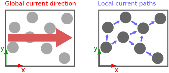
Figure 7 Directions of local current flow in a hexagonal particle arrangement. For a global current in the x direction, particle-to-particle currents have an x and y component, leading to transverse sensitivity.

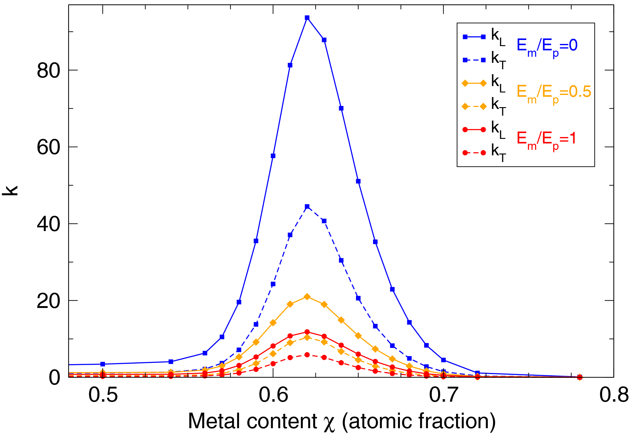
Figure 8 Longitudinal and transverse gauge factors for different elastic moduli of matrix (E_m) and particles (E_p). Blue: $E_{\mathrm{m}}=\mathrm{0},E_{\mathrm{p}}>\mathrm{0}$. Orange: $E_{\mathrm{m}}=E_{\mathrm{p}}/\mathrm{2}$. Red: E_m=E_p.

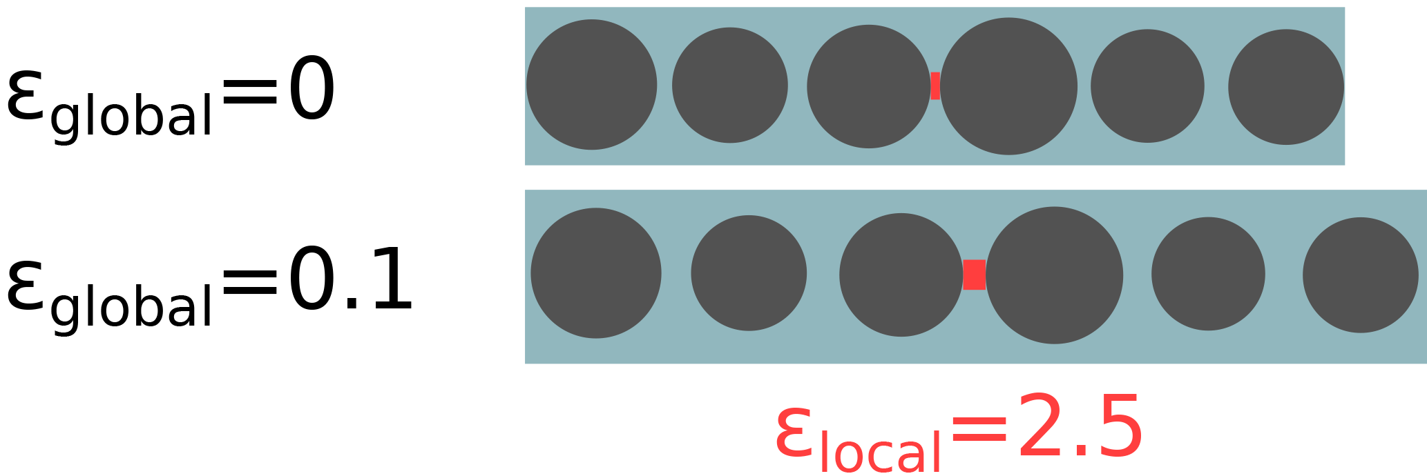
Figure 9 Mechanical strain enhancement for incompressible metal particles, i.e., $E_{\mathrm{m}}/E_{\mathrm{p}}=\mathrm{0}$ (exaggerated example).

The changes in the k(s) curve shape occur because – as can be seen in the resistance law – there is an optimum distance s. For the σ_d=0 plot and the right value of metal content, this optimum s and thus the maximum possible k_L are achieved. In the films with a certain geometrical disorder, there is no fixed s, but a normal distribution of s values. All individual smaller and larger s will contribute to a reduction of k_L, therefore, for a larger σ_d, the maximum k_L becomes smaller. While the maximum is reduced, the region of increased gauge factors is widened with growing σ_d. The reason can be seen when we consider the data points at s=3 nm with σ_d=0 and all distances s in the film are far from the optimum of the resistance law and the gauge factor is only 2. With σ_d=1 nm, the mean value of s is the same; however, due to the underlying distribution, half of the distances are larger and half are smaller than that. All smaller distances in the distribution correspond to inter-particle links with a higher gauge factor so that the gauge factor is effectively increased compared to the perfectly ordered film for this value of s.

The results show that even for a hexagonal grid without any disorder in diameter (σ_d=0), a transverse sensitivity of $k_{\mathrm{T}}/k_{\mathrm{L}}\approx \mathrm{0.33}$ occurs. This is due to the fact that in our implementation (as in the actual thin film) the system has no preferred directions in its particle-to-particle paths and usually no straight paths all the way through the film in the x direction. Conduction paths naturally follow various detours in the y direction, as can be seen in Fig. 7. When the film is strained transverse to the current direction, these components of the conduction paths result in a resistance change, which we describe as the transverse gauge factor k_T.

With a growing disorder due to varying diameters, the transverse sensitivity is enhanced, because detours within the possible conduction paths are becoming increasingly favorable. Since straight paths are more and more likely to contain some increased separating distances, detours along shorter separating distances become more viable.

It becomes apparent that a transverse sensitivity ratio of $k_{\mathrm{T}}/k_{\mathrm{L}}=\mathrm{1}/\mathrm{3}$ is the lower limit for a film of two-dimensional hexagonal (and possibly for non-ordered) packing. All disorder in particle distances further increases the transverse sensitivity. At the same time, disorder widens the comparably sharp peaks: with disorder, a larger range of metal content has an increased k_L, albeit with a smaller maximum value.

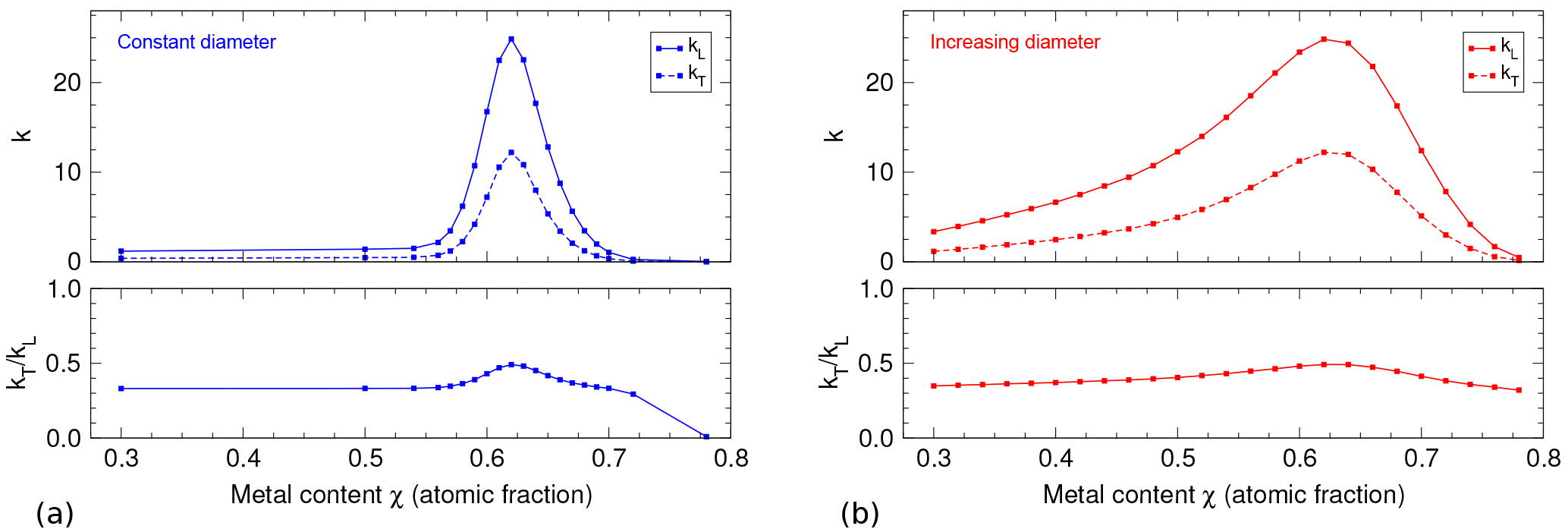
Figure 10 Gauge factors k_L and k_T over metal fraction for (a) constant and (b) increasing column diameter. With increasing diameters, the area of elevated gauge factors stretches across a wider range of metal content.

4.2 Influence of elastic moduli

The influence of elastic moduli of matrix (E_m) and metal particles (E_p) is shown in Fig. 8. Changes in elastic moduli do not shift the curves with increasing metal content χ – the maximum remains in the presented case at 0.64. With an increasing elastic modulus of the matrix material, gauge factors are suppressed equally so that the transverse sensitivity ratio k_T∕k_L remains constant. The maximum possible gauge factors are strongly affected: max(k_L) is reduced from 94 to 12 when comparing $E_{\mathrm{m}}/E_{\mathrm{p}}=\mathrm{0}$ to $E_{\mathrm{m}}/E_{\mathrm{p}}=\mathrm{1}$.

The underlying effect is a mechanical and geometrical one: for $E_{\mathrm{m}}/E_{\mathrm{p}}=\mathrm{0}$, all deformation has to be absorbed by the matrix sections between particles, while the metal particles themselves are not strained at all; this leads to a local strain enhancement to values well above the globally applied strain, as schematically shown in Fig. 9. With equal moduli, $E_{\mathrm{m}}/E_{\mathrm{p}}=\mathrm{1}$, strain is homogeneous: the strain between particles is equal to the global strain (no strain enhancement). Depending on the material combination, with $E_{\mathrm{m}}/E_{\mathrm{p}}>\mathrm{1}$ the opposite effect, i.e., a local strain reduction, could occur as well and further reduce the possible gauge factors.

4.3 Column diameter influence

The column diameter of about 15 nm described before was found for one particular nickel–carbon film. For the samples with lower or higher metal content, the column diameter is unknown. Because of the uncertainties in the precise structure and geometry of the films, we present some typical simulation results for different assumptions regarding the dependence of particle size on metal content. They can be evaluated quantitatively regarding the longitudinal and transverse gauge factors, but only qualitatively in their dependence on particle separation, diameter, and metal content.

4.3.1 Example 1: constant diameter

If we assume a constant column diameter for all values of metal content χ, the separating distance s is reduced with growing metal content and we find the characteristic k(χ) curve shown in Fig. 10a. With $b=\mathrm{1}\times {\mathrm{10}}^{-\mathrm{9}}\mathrm{\Omega }$, $c=\mathrm{11}{\mathrm{nm}}^{-\mathrm{1}}$, and $E_{\mathrm{m}}/E_{\mathrm{p}}=\mathrm{80}$ GPa∕200 GPa = 0.4, the simulation exhibits characteristics evidenced by experiments: with growing metal content, k_L shows a rapid increase around 50 at. % metal, a maximum in the [50–60] at. % interval and a slightly slower decrease until about 75 at. %. The transverse sensitivity is highest when k_L reaches its maximum. The experimental value of $k_{\mathrm{T}}/k_{\mathrm{L}}\approx \mathrm{0.5}$ is reproduced with ${\mathit{\sigma }}_d={\mathit{\sigma }}_s=\mathrm{0.35}\mathrm{nm}$.

4.3.2 Example 2: diameter increasing with metal content

Results by El Mel et al. (2012) and Zohar-Hauber (2012) indicate that the size of metal particles in sputter-deposited nickel–carbon films depends on the metal content nonlinearly. With higher metal content, larger particles grow. Based on our results, we assume that the particle size for the relevant metal fractions of about 50 to 70 at. % varies between 10 and 20 nm. With these given points, we use an exponential function as a simple model for the variable column diameter:

$$\begin{array}{}\text{(10)}& {\displaystyle }{\displaystyle }d\left(\mathit{\chi }\right)=c_{\mathrm{1}}\cdot e^{c_{\mathrm{2}}\cdot \mathit{\chi }},c_{\mathrm{1}}=\mathrm{1.76}\mathrm{nm},c_{\mathrm{2}}=\mathrm{3.47}.\end{array}$$

In Fig. 10b, the simulation parameters are identical, but the diameter changes with metal content. The assumption of varying diameter is based on results from literature. In results, the k(χ) curve has a less sharp peak and is stretched along a wider range of χ values. The underlying k(s) resistance law is still the same but due to the change in diameter d(x), the change of s with metal content χ is modified; for a small metal fraction, the diameter is small; for an increasing metal fraction, diameters increase as well. This results in a slower change of particle separation s, so favorable values of s – and consequently increased gauge factors – stretch across a wider range of metal fractions.

Compared to the constant-diameter example, this result better reflects our experiments (Schultes et al., 2018; Fig. 6) because a gauge factor maximum is found at about 60 at. % metal. At higher metal content, the gauge factor drops relatively quickly; towards lower metal content, the decrease is slower. The simulation shows a transverse sensitivity ratio k_T∕k_L that still has a maximum of 0.5 at the maximum gauge factor k_L and is lower for lower gauge factors, but its peak is stretched as well.

Still, the gauge factors obtained experimentally for low metal content (χ<0.4) are not reproduced by the model. This is likely due to the gauge factor of the carbon matrix itself (without metal), which is not represented in our model.

5 Conclusions and outlook

An experimentally found characteristic of our nickel–carbon films is a gauge factor maximum vs. metal content with a relatively wide range of elevated gauge factors. At the same time, a substantial transverse sensitivity ratio in the range of 0.5 is seen. These general properties are reproduced by simulations of the strain sensitivity for a relative SD of tunneling distances of about 10 %.

The base value of the transverse sensitivity ratio for a film in a two-dimensional, perfectly hexagonal particle arrangement is $k_{\mathrm{T}}/k_{\mathrm{L}}=\mathrm{1}/\mathrm{3}$. Any disorder in particle separation distances increases this ratio. Different arrangements, such as a rectangular grid of particles could reduce transverse sensitivity, but seem experimentally unlikely for our sputtering process. Our films exhibit unordered close packing with separation walls of similar thickness between metal columns and no preferred directions.

The model highlights the possible gauge factor enhancement caused by mechanical properties of the matrix material: with a relatively low elastic modulus of matrix vs. metal particles, significant local strain enhancement will occur. This amplified change in separation distance will result in a larger gauge factor k_L, while k_T will grow proportionally and the transverse sensitivity ratio remains the same.

As has been found experimentally before, the model shows that the particle separation distances should be carefully tuned by choice of metal content to achieve the optimum of possible gauge factors. The simulated k_L(x) curve is in qualitative agreement with experiments, however, quantitative comparison is difficult because the detailed structure (column diameters, separation distances, and their distributions) requires extensive characterization to determine. An extremely detailed sample characterization for a series of samples would be required, because changes in a single sputtering parameter, i.e., ethylene gas flow, will alter a number of film parameters. For a more detailed model evaluation, this highlights the need to perform further experiments including not only gauge factor measurements of films with different metal content but also a comprehensive structural and geometrical analysis of the same films.