Inductive localization accuracy of a passive 3-D coil in an Industry 4.0 environment

In this paper a localization system of a passive 3-D coil is proposed and signal uncertainties due to the 3-D coil's arbitrary orientation are analyzed. The 3-D coil is excited by an alternating primary magnetic field. Geometrically distributed pick-up coils measure the 3-D coil's secondary field. By means of a simulated look-up table that assigns expected voltages from the pick-up coils to the positions of the 3-D coil, the position of the 3-D coil is deduced by a least-squares approach. A basic assumption is that the secondary field is invariant to the orientation of the 3-D coil. This allows a reduction of the computational effort for the look-up table generation and the table search during the localization phase since for each position the field distribution for only one orientation has to be calculated. However, the assumption of invariance to rotation is only valid for a dipole model. In this paper we investigate the localization error introduced by this assumption when using 3-D coils with a geometric extent in an inhomogeneous primary field. Optimized localization methods that decrease the statistical error are proposed. The theoretical results are verified with measurements conducted on a laboratory system.

1 Introduction

Nearly every modern producing industry has a storage solution within their logistics process. The most flexible way for picking items from a shelf is still by human interaction. However, cost-intensive errors can occur when a storekeeper picks an item from the wrong shelf. It is important to provide a technology that gives the operator feedback in case of a wrong pick. Several technologies already exist to support the operator. In pick-by-light systems the shelf or container from which an item has to be picked is illuminated (Baechler et al., 2016). The pick-by-vision approach provides the user with an augmented reality view of the storage using a head-mounted display (Schwerdtfeger et al., 2009; Guo et al., 2015). Solutions with scales below each container are proposed in KBS (2018a). Audio systems that guide the operator are described in Starner (2002). As an alternative or extension, camera-based systems can provide important feedback to the operator in case of a wrongly picked item (KBS, 2018b). Such solutions, however, require a line of sight. Also, dirt, fog or bad lighting conditions from the harsh industrial environment can degrade the performance. The industry needs a solution that can localize the hand of the operator in a robust and reliable way.

In this paper we propose a magnetic-field-based approach for the localization of an operator's hand in a shelf. The advantage of the magnetic approach is that no direct line of sight is necessary and the installation costs are relatively low. The estimation of the position and the orientation of a magnetic source based on measured field values is a classic inverse problem. The corresponding direct problem is the calculation of a field distribution knowing the position, orientation and strength of the field sources, which can be done using Maxwell's equations. The inverse problem, however, is often ill-posed. That means it can have no solution or multiple solutions or that the solution can be very sensitive to noisy data. In order to account for that, regularization techniques are used (Vogel, 2002).

Several methods exist for the estimation of the position and the orientation of a magnetic field source. The straightforward approach to estimate the position of a field source is to compare a measured magnetic field distribution at several points in space to a theoretical field distribution that is calculated by means of a mathematical model for a certain position and orientation of the field source. Analytical approaches as described in Nara et al. (2006) can estimate the position of a magnetic dipole with a magnetic moment whose norm is constant. This method is obviously based on a simple magnetic dipole model. Also, it is very sensitive to noise. In Neudeck et al. (2016) the position and orientation of a rectangular magnet are estimated. Due to the rectangular shape of the magnet the model is more sophisticated and two additional degrees of freedom for the orientation can be estimated. A Levenberg–Marquardt optimization algorithm is used to optimize the fit between the theoretical field distribution from the model and the measured fields. An advantage of using an optimization-based approach is that not all possible combinations of positions and orientations of the magnet need to be calculated. This comes with the risk of sticking to local solutions or even divergence of the estimate (Brauer et al., 2006). Of course, as proposed by Moreno and Skarmeta (2015) and Heinig et al. (2010) a set of measurements of a real field distribution can be used instead of a theoretical model. Such fingerprinting methods have their advantage when the field distribution is too complicated to be modeled mathematically, e.g., when too many constant disturbances are located in the area of interest. The disadvantage is that the method degrades as the environment changes. To still be able to localize the object, a new time-consuming measurement of the field distribution must be performed. Localizing an active coil over a distance in the meter range is presented in Arumugam et al. (2013). The applied model is again a dipole model but extended by a term that utilizes the influence of the soil on the magnetic field. The authors use a least-squares optimization algorithm to find the global solution.

All of the above methods need an active magnetic field source which they mostly approximate by a simple dipole model. In contrast, we utilize a passive field source, whose equivalent magnetic dipole moment is additionally position dependent. Furthermore the model we utilize is more sophisticated and takes the geometry of the current paths into account. The approach we present in this paper is based on the GoalRef technology (Psiuk et al., 2014), which is a magnetic-field-based goal detection system for professional football. The FIFA (Fédération Internationale de Football Association)-certified technology measures the disturbance of an artificial magnetic field that occurs due to resonantly tuned coils built into the football. The traditional GoalRef system has been able to only detect transitions through the goal plane without providing further information about the ball's position.

For the adaption of that technology to our localization approach for logistics, the new proposed system is extended with the ability to localize a passive 3-D coil in three space dimensions in the proximity of a shelf. Therefore a primary current loop is positioned around that shelf, which generates a primary magnetic field. The field induces a current in a passive resonantly tuned 3-D coil that is mounted on the hand of the operator. That current flow in turn generates a secondary magnetic field that is measured by pick-up coils around the shelf. From voltage measurements at these pick-up coils the position of the 3-D coil is deduced by utilizing a look-up table that is generated by the forward model presented in Psiuk et al. (2017a). Since only the position of the hand and not its orientation is of interest, three perpendicular passive coils are used as a localization object instead of a single coil. By doing this the dependence of the secondary field on the orientation of the hand is reduced drastically. However, the dependence is not completely removed and still influences the localization result. Neither to what extent the measured fields are influenced by the arbitrary orientation nor how in a subsequent step that uncertainty in the measured signals affects the localization has been investigated yet. In this paper we investigate the remaining localization error due to the orientation dependence of the measured field. First we identify the sources of signal uncertainty. Then we quantify their contribution to the overall signal variation analytically. Afterwards the localization error due to those signal uncertainties is compared for different localization methods. For reduced complexity the investigations are carried out on a simplified setup for a 1-D position estimation.

The paper is structured as follows. In Sect. 2 the system and the general localization method are presented. The uncertainty of the measured magnetic field due to the orientation of the hand is derived in Sect. 3. In Sect. 4 several localization methods are introduced. The theoretical accuracy of different localization approaches is compared through simulations in Sect. 5. Measurements that verify the simulations are shown in Sect. 6. The results are discussed in Sect. 7, and Sect. 8 concludes the paper.

2 Employed methods

In this section the experimental system setup and the basic localization method are explained.

2.1 Experimental setup

Similarly to an LF RFID (low-frequency radio frequency identification) system, our setup includes a reader that generates a continuous low-frequency current in a primary exciter wire loop around a shelf as depicted in Fig. 1. That current flow leads, according to Ampère's law, to a magnetic field in phase with the current. The localization object bears three passive coils as shown in Fig. 2. The passive coils are tuned by means of capacitors to form a resonant circuit whose resonance frequency coincides with the excitation frequency. Due to Faraday's law a voltage and hence a current flow are induced in the three coils. That current leads to a secondary magnetic field that is measured with pick-up coils mounted around the shelf. The measured field from the pick-up coils is then led back to the reader, where analog and digital signal processing is performed. The processed signals are forwarded to a personal computer where the position estimation algorithms are running in the Python programming language (Psiuk et al., 2017b).

Figure 1 Shelf with the exciter wire, eight pick-up coils around the shelf and a 3-D coil in one compartment.

Figure 2 3-D coil with three passive resonantly tuned individual windings.

2.2 Proposed localization method

Different optimization algorithms as described in Sect. 1 might show varying behavior concerning convergence towards the global solution. Therefore the localization accuracy would depend on the particular method being used. In our investigations we are interested in the accuracy independent of the specific algorithm in use. As a basis localization method we therefore localize by means of a global search in a look-up table containing simulated field values. Measured field values are compared to the entries in the table. That particular position and orientation entry in the table is selected as an estimate whose corresponding field values show the best agreement with the measured field values using a least-squares approach as proposed by Arumugam et al. (2013). The table is created to contain field values for positions of the localization object in a regular grid with a sufficiently high resolution not to influence the results of our analyses.

In our system the magnetic field strength of the localization object depends on the object's position and orientation. Thus, a sophisticated mathematical system model is needed to address that behavior. Such a model has been presented in Psiuk et al. (2017a). Using the law of Biot–Savart, the model is capable of calculating the magnetic flux density vector field and the magnetic vector potential of arbitrarily shaped current-carrying wire constellations. The model can also calculate induced voltages in closed loops and hence the induced current in arbitrarily shaped coils, based on the law of Faraday and the previously calculated vector fields. On the basis of these operations the induced voltages in pick-up coils around the shelf can be calculated for a series of positions and orientations of the localization object and hence the localization look-up table described above can be generated.

If only a single coil was mounted on the localization object, a look-up table would need to include three entries for three dimensions of position and two dimensions of orientation. The third rotational degree of freedom is omitted due to rotation symmetry of a circular coil. Such a table with a fine enough grid to provide a good estimation accuracy to be generated in practice would require a high computational effort. Also, searching the whole table for the globally best solution with each localization step would take a long time, which makes real-time applications difficult. Another disadvantage of localizing only one passive coil in a primary magnetic field is that for any coil position there are orientations at which the coil is orthogonal to the primary field and hence cannot develop a secondary field. A localization would not be possible in such a case.

Since we are not interested in the orientation but only in the position of the object, we propose an approach that makes the localization computationally less expensive. Instead of using only one coil, we use a coil system comprising three passive orthogonal coils. The basic assumption is that the three coils provide an equivalent secondary magnetic moment m that only marginally depends on the orientation of the coil system. This way for a certain position only one orientation of the 3-D coil needs to be considered for the localization table, which greatly reduces the computational effort in creating the look-up table as well as the computational effort in searching in it. Another advantage is that at least one of the three coils always produces a secondary magnetic field at any position independent of the orientation.

3 Orientation-induced uncertainty of the secondary magnetic field

The reduced-complexity method described in Sect. 2.2 relies on the assumption that the secondary field of the 3-D coil system does not depend on its orientation. However, this is only approximately true. In this section we investigate the theoretical accuracy degradation due to this model simplification. First, the basic assumption of the theoretical rotation invariance of the secondary field is proven for three orthogonal dipoles in a homogeneous primary field. Then the contributions of the 3-D coil's geometry and the primary field's inhomogeneity to the voltage distribution in a pick-up coil are investigated.

3.1 Orientation-independent secondary magnetic field

This section verifies analytically the assumption of the rotation-invariant secondary equivalent magnetic dipole field of a 3-D coil in a homogeneous primary magnetic field. In the following, complex values are underlined, the hat superscript stands for a peak value and the superscripts l and g on variables indicate the coordinate system in which they are expressed, where l stands for the local coordinate system of the moving 3-D coil and g for the fixed global coordinate system.

Let us assume a system comprising three orthogonal circular coils, all with the same radius a and N windings. The center of each coil is in the global coordinate system's origin. In the initial state the local and global coordinate systems coincide. The equivalent area normal vectors S_i of the planes spanned by each coil are

$$\begin{array}{}\text{(1)}& {\mathit{S}}_i^{\mathrm{l}}=N\mathit{\pi }{a}^{\mathrm{2}}{\mathit{e}}_i^{\mathrm{l}}\text{with}i\in \left\{\mathrm{1},\mathrm{2},\mathrm{3}\right\},\end{array}$$

where ${\mathit{e}}_i^{\mathrm{l}}$ are the unity direction vectors of each of the three area normal vectors. The area normal vectors of the coils point each to one of the three positive local Cartesian coordinates x, y and z. The area normal vector of coil 1 points in the x direction, the one of coil 2 points in the y direction and the one of coil 3 points in the z direction of the local coordinate system:

$$\begin{array}{}\text{(2)}& {\displaystyle }{\mathit{e}}_{\mathrm{1}}^{\mathrm{l}}={\left(\begin{array}{ccc}\mathrm{1}& \mathrm{0}& \mathrm{0}\end{array}\right)}^{\mathrm{T}},{\mathit{e}}_{\mathrm{2}}^{\mathrm{l}}={\left(\begin{array}{ccc}\mathrm{0}& \mathrm{1}& \mathrm{0}\end{array}\right)}^{\mathrm{T}},{\mathit{e}}_{\mathrm{3}}^{\mathrm{l}}={\left(\begin{array}{ccc}\mathrm{0}& \mathrm{0}& \mathrm{1}\end{array}\right)}^{\mathrm{T}}.\end{array}$$

We assume a homogeneous primary magnetic flux density ${\underset{\mathrm{¯}}{\mathit{B}}}_{\mathrm{p}}^{\mathrm{g}}$ with a peak value of ${\underset{\mathrm{¯}}{\widehat{\mathit{B}}}}_{\mathrm{p}}^{\mathrm{g}}$, which, without loss of generality, points in the global z direction:

$$\begin{array}{}\text{(3)}& {\underset{\mathrm{¯}}{\widehat{\mathit{B}}}}_{\mathrm{p}}^{\mathrm{g}}={\left(\begin{array}{ccc}\mathrm{0}& \mathrm{0}& {\underset{\mathrm{¯}}{\widehat{B}}}_z\end{array}\right)}^{\mathrm{T}}.\end{array}$$

With the three rotation matrices

$$\begin{array}{ll}{\displaystyle }& {\displaystyle }{\mathbf{R}}_x\left(\mathrm{\Phi }\right)=\left(\begin{array}{ccc}\mathrm{1}& \mathrm{0}& \mathrm{0}\\ \mathrm{0}& \cos \left(\mathrm{\Phi }\right)& \sin \left(\mathrm{\Phi }\right)\\ \mathrm{0}& -\sin \left(\mathrm{\Phi }\right)& \cos \left(\mathrm{\Phi }\right)\end{array}\right),\\ {\displaystyle }& {\displaystyle }{\mathbf{R}}_y\left(\mathrm{\Theta }\right)=\left(\begin{array}{ccc}\cos \left(\mathrm{\Theta }\right)& \mathrm{0}& -\sin \left(\mathrm{\Theta }\right)\\ \mathrm{0}& \mathrm{1}& \mathrm{0}\\ \sin \left(\mathrm{\Theta }\right)& \mathrm{0}& \cos \left(\mathrm{\Theta }\right)\end{array}\right),\\ \text{(4)}& {\displaystyle }& {\displaystyle }{\mathbf{R}}_z\left(\mathrm{\Psi }\right)=\left(\begin{array}{ccc}\cos \left(\mathrm{\Psi }\right)& \sin \left(\mathrm{\Psi }\right)& \mathrm{0}\\ -\sin \left(\mathrm{\Psi }\right)& \cos \left(\mathrm{\Psi }\right)& \mathrm{0}\\ \mathrm{0}& \mathrm{0}& \mathrm{1}\end{array}\right),\end{array}$$

and their combination

$$\begin{array}{}\text{(5)}& \mathbf{R}(\mathrm{\Psi },\mathrm{\Theta },\mathrm{\Phi })={\mathbf{R}}_x\left(\mathrm{\Phi }\right)\cdot {\mathbf{R}}_y\left(\mathrm{\Theta }\right)\cdot {\mathbf{R}}_z\left(\mathrm{\Psi }\right),\end{array}$$

the 3-D coil's local coordinate system can be rotated in space against the global coordinate system. First the local coordinate system is rotated around the global z axis by the angle Ψ (yaw), and then it is rotated around the y axis of the new local coordinate system by the angle Θ (pitch) and finally around the x axis of the new local coordinate system by the angle Φ (roll). Applying Eq. (5) to Eq. (3), the primary magnetic flux density vector field can be expressed in local coordinates as

$$\begin{array}{}\text{(6)}& {\underset{\mathrm{¯}}{\widehat{\mathit{B}}}}_{\mathrm{p}}^{\mathrm{l}}(\mathrm{\Psi },\mathrm{\Theta },\mathrm{\Phi })=\mathbf{R}(\mathrm{\Psi },\mathrm{\Theta },\mathrm{\Phi })\cdot {\underset{\mathrm{¯}}{\widehat{\mathit{B}}}}_{\mathrm{p}}^{\mathrm{g}}.\end{array}$$

The primary magnetic flux ${\underset{\mathrm{¯}}{\widehat{\mathrm{\Phi }}}}_i$ through each of the three coils can be calculated by

$$\begin{array}{}\text{(7)}& {\underset{\mathrm{¯}}{\widehat{\mathrm{\Phi }}}}_i(\mathrm{\Psi },\mathrm{\Theta },\mathrm{\Phi })={\underset{\mathrm{¯}}{\widehat{\mathit{B}}}}_{\mathrm{p}}^{\mathrm{l}}(\mathrm{\Psi },\mathrm{\Theta },\mathrm{\Phi })\cdot {\mathit{S}}_i^{\mathrm{l}}.\end{array}$$

According to Faraday's law of induction, the resulting induced current flow ${\underset{\mathrm{¯}}{\widehat{i}}}_i$ in each of the coils is

$$\begin{array}{}\text{(8)}& {\underset{\mathrm{¯}}{\widehat{i}}}_i(\mathrm{\Psi },\mathrm{\Theta },\mathrm{\Phi })={\displaystyle \frac{-j\mathrm{2}\mathit{\pi }f{\underset{\mathrm{¯}}{\widehat{\mathrm{\Phi }}}}_i(\mathrm{\Psi },\mathrm{\Theta },\mathrm{\Phi })}{\underset{\mathrm{¯}}{Z}}},\end{array}$$

where j is the imaginary number, f is the frequency of the time-varying field ${\underset{\mathrm{¯}}{\mathit{B}}}_{\mathrm{p}}^{\mathrm{g}}$ and $\underset{\mathrm{¯}}{Z}$ is the complex impedance of the coil (Lehner, 2010). With the currents ${\underset{\mathrm{¯}}{\widehat{i}}}_i$ the equivalent magnetic dipole moment ${\underset{\mathrm{¯}}{\widehat{\mathit{m}}}}^{\mathrm{g}}$ of the 3-D coil can be calculated by

$$\begin{array}{}\text{(9)}& {\underset{\mathrm{¯}}{\widehat{\mathit{m}}}}^{\mathrm{g}}={\mathbf{R}}^{-\mathrm{1}}\sum _{i=\mathrm{1}}^{\mathrm{3}}{\underset{\mathrm{¯}}{\widehat{\mathit{m}}}}_i^{\mathrm{l}}={\mathbf{R}}^{\mathrm{T}}\sum _{i=\mathrm{1}}^{\mathrm{3}}{\underset{\mathrm{¯}}{\widehat{\mathit{m}}}}_i^{\mathrm{l}}\text{with}{\underset{\mathrm{¯}}{\widehat{\mathit{m}}}}_i^{\mathrm{l}}={\underset{\mathrm{¯}}{\widehat{i}}}_i{\mathit{S}}_i^{\mathrm{l}}.\end{array}$$

Since rotation matrices are orthogonal matrices, their inverse R⁻¹ is also their transpose R^T (Bronshtein et al., 2004). Solving Eq. (9) shows that the magnetic dipole moment ${\underset{\mathrm{¯}}{\widehat{\mathit{m}}}}^{\mathrm{g}}$ does not depend on any of the orientation angles Ψ, Θ and Φ:

$$\begin{array}{}\text{(10)}& {\underset{\mathrm{¯}}{\widehat{\mathit{m}}}}^{\mathrm{g}}={\left(\begin{array}{ccc}\mathrm{0}& \mathrm{0}& \frac{-j\mathrm{2}{\mathit{\pi }}^{\mathrm{3}}f{\underset{\mathrm{¯}}{\widehat{B}}}_z{N}^{\mathrm{2}}{a}^{\mathrm{4}}}{\underset{\mathrm{¯}}{Z}}\end{array}\right)}^{\mathrm{T}}.\end{array}$$

The secondary magnetic flux density ${\underset{\mathrm{¯}}{\widehat{\mathit{B}}}}_{\mathrm{d}}^{\mathrm{g}}$ of the 3-D coil modeled as a dipole can be calculated at the position ${\mathit{r}}^{\mathrm{g}}=(x,y,z{)}^{\mathrm{T}}$ by

$$\begin{array}{}\text{(11)}& {\underset{\mathrm{¯}}{\widehat{\mathit{B}}}}_{\mathrm{d}}^{\mathrm{g}}({\underset{\mathrm{¯}}{\widehat{\mathit{m}}}}^{\mathrm{g}},{\mathit{r}}^{\mathrm{g}})={\displaystyle \frac{{\mathit{\mu }}_{\mathrm{0}}\left(\mathrm{3}({\underset{\mathrm{¯}}{\widehat{\mathit{m}}}}^{\mathrm{g}}\cdot \mathit{n})\mathit{n}-{\underset{\mathrm{¯}}{\widehat{\mathit{m}}}}^{\mathrm{g}}\right)}{\mathrm{4}\mathit{\pi }{r}^{\mathrm{3}}}},\end{array}$$

where μ₀ is the vacuum permeability, r=|r^g| and $\mathit{n}={\mathit{r}}^{\mathrm{g}}/r$ (Nara et al., 2006). Inserting Eq. (10) into Eq. (11) results in the orientation-invariant secondary magnetic flux density

$$\begin{array}{}\text{(12)}& {\underset{\mathrm{¯}}{\widehat{\mathit{B}}}}_{\mathrm{d}}^{\mathrm{g}}={\displaystyle \frac{j{a}^{\mathrm{4}}{\underset{\mathrm{¯}}{\widehat{B}}}_{z}f{N}^{\mathrm{2}}{\mathit{\mu }}_{\mathrm{0}}{\mathit{\pi }}^{\mathrm{2}}}{\mathrm{2}\underset{\mathrm{¯}}{Z}}}\left(\begin{array}{c}-\frac{\mathrm{3}xz}{r^{\mathrm{5}}}\\ -\frac{\mathrm{3}yz}{r^{\mathrm{5}}}\\ \frac{x^{\mathrm{2}}+y^{\mathrm{2}}-\mathrm{2}{z}^{\mathrm{2}}}{r^{\mathrm{5}}}\end{array}\right).\end{array}$$

Equation (12) shows that, assuming a homogeneous primary magnetic field and a magnetic dipole model for the individual coils, the orientation of the 3-D coil has no influence on the secondary magnetic field distribution.

3.2 Coil-geometry-induced secondary field uncertainty

In the practical case two assumptions made in Sect. 3.1 do not apply; on the one hand coils do have a certain physical extent in contrast to theoretical magnetic dipoles and on the other hand the primary field is not necessarily homogeneous. In order to analyze both assumptions separately we first keep the assumption of a homogeneous primary magnetic field but replace the dipole model with a circular coil model. For the calculation of the induced currents ${\underset{\mathrm{¯}}{\widehat{i}}}_i$, Eq. (8) can still be applied. The secondary magnetic flux density ${\underset{\mathrm{¯}}{\widehat{\mathit{B}}}}_{\mathrm{c}}^{\mathrm{l}}$ of a circular loop that is centered and aligned with the coordinate system axes differs from the field of a dipole as described by Simpson et al. (2001):

$$\begin{array}{}\text{(13)}& {\underset{\mathrm{¯}}{\widehat{\mathit{B}}}}_{\mathrm{c}}^{\mathrm{l}}=\left(\begin{array}{c}{\underset{\mathrm{¯}}{\widehat{B}}}_{\mathrm{c},x}^{\mathrm{l}}\\ {\underset{\mathrm{¯}}{\widehat{B}}}_{\mathrm{c},y}^{\mathrm{l}}\\ {\underset{\mathrm{¯}}{\widehat{B}}}_{\mathrm{c},z}^{\mathrm{l}}\end{array}\right),\end{array}$$

with

$$\begin{array}{}\text{(14)}& {\displaystyle }& {\displaystyle }{\underset{\mathrm{¯}}{\widehat{B}}}_{\mathrm{c},x}^{\mathrm{l}}={\displaystyle \frac{{\mathit{\mu }}_{\mathrm{0}}{\underset{\mathrm{¯}}{\widehat{i}}}_{i}xz}{\mathrm{2}\mathit{\pi }{\mathit{\alpha }}^{\mathrm{2}}\mathit{\beta }{\mathit{\rho }}^{\mathrm{2}}}}\left[\left(a^{\mathrm{2}}+r^{\mathrm{2}}\right)E\left(k^{\mathrm{2}}\right)-{\mathit{\alpha }}^{\mathrm{2}}K\left(k^{\mathrm{2}}\right)\right],\text{(15)}& {\displaystyle }& {\displaystyle }{\underset{\mathrm{¯}}{\widehat{B}}}_{\mathrm{c},y}^{\mathrm{l}}={\displaystyle \frac{y{\underset{\mathrm{¯}}{\widehat{B}}}_{\mathrm{c},x}^{\mathrm{l}}}{x}},\text{(16)}& {\displaystyle }& {\displaystyle }{\underset{\mathrm{¯}}{\widehat{B}}}_{\mathrm{c},z}^{\mathrm{l}}={\displaystyle \frac{{\mathit{\mu }}_{\mathrm{0}}{\underset{\mathrm{¯}}{\widehat{i}}}_i}{\mathrm{2}\mathit{\pi }{\mathit{\alpha }}^{\mathrm{2}}\mathit{\beta }}}\left[\left(a^{\mathrm{2}}-r^{\mathrm{2}}\right)E\left(k^{\mathrm{2}}\right)+{\mathit{\alpha }}^{\mathrm{2}}K\left(k^{\mathrm{2}}\right)\right],\end{array}$$

and

$$\begin{array}{}\text{(17)}& {\displaystyle }& {\displaystyle }{\mathit{\rho }}^{\mathrm{2}}=x^{\mathrm{2}}+y^{\mathrm{2}},\text{(18)}& {\displaystyle }& {\displaystyle }{r}^{\mathrm{2}}=x^{\mathrm{2}}+y^{\mathrm{2}}+z^{\mathrm{2}},\text{(19)}& {\displaystyle }& {\displaystyle }{\mathit{\alpha }}^{\mathrm{2}}=a^{\mathrm{2}}+r^{\mathrm{2}}-\mathrm{2}a\mathit{\rho },\text{(20)}& {\displaystyle }& {\displaystyle }{\mathit{\beta }}^{\mathrm{2}}=a^{\mathrm{2}}+r^{\mathrm{2}}+\mathrm{2}a\mathit{\rho },\text{(21)}& {\displaystyle }& {\displaystyle }{k}^{\mathrm{2}}=\mathrm{1}-{\mathit{\alpha }}^{\mathrm{2}}/{\mathit{\beta }}^{\mathrm{2}},\end{array}$$

including the complete elliptical integrals of the first and second kinds K(⋅) and E(⋅), respectively. The secondary field ${\underset{\mathrm{¯}}{\widehat{\mathit{B}}}}_{{\mathrm{c}}_i}^{\mathrm{g}}$ of each rotated coil c_i at the global position r can be calculated by

$$\begin{array}{}\text{(22)}& {\displaystyle }& {\displaystyle }{\underset{\mathrm{¯}}{\widehat{\mathit{B}}}}_{{\mathrm{c}}_{\mathrm{1}}}^{\mathrm{g}}={\left({\mathbf{R}}_y(\mathit{\pi }/\mathrm{2})\cdot {\mathbf{R}}^{\mathrm{T}}\right)}^{\mathrm{T}}\cdot {\underset{\mathrm{¯}}{\widehat{\mathit{B}}}}_{{\mathrm{c}}_{\mathrm{1}}}^{\mathrm{l}}\left({\mathbf{R}}_y(\mathit{\pi }/\mathrm{2})\cdot {\mathbf{R}}^{\mathrm{T}}\cdot \mathit{r}\right),\text{(23)}& {\displaystyle }& {\displaystyle }{\underset{\mathrm{¯}}{\widehat{\mathit{B}}}}_{{\mathrm{c}}_{\mathrm{2}}}^{\mathrm{g}}={\left({\mathbf{R}}_x(-\mathit{\pi }/\mathrm{2})\cdot {\mathbf{R}}^{\mathrm{T}}\right)}^{\mathrm{T}}\cdot {\underset{\mathrm{¯}}{\widehat{\mathit{B}}}}_{{\mathrm{c}}_{\mathrm{2}}}^{\mathrm{l}}\left({\mathbf{R}}_x(-\mathit{\pi }/\mathrm{2})\cdot {\mathbf{R}}^{\mathrm{T}}\cdot \mathit{r}\right),\text{(24)}& {\displaystyle }& {\displaystyle }{\underset{\mathrm{¯}}{\widehat{\mathit{B}}}}_{{\mathrm{c}}_{\mathrm{3}}}^{\mathrm{g}}=\mathbf{R}\cdot {\underset{\mathrm{¯}}{\widehat{\mathit{B}}}}_{{\mathrm{c}}_{\mathrm{3}}}^{\mathrm{l}}\left({\mathbf{R}}^{\mathrm{T}}\cdot \mathit{r}\right).\end{array}$$

For the secondary magnetic flux density of a circular 3-D coil follows

$$\begin{array}{}\text{(25)}& {\underset{\mathrm{¯}}{\widehat{\mathit{B}}}}_{\mathrm{c}}^{\mathrm{g}}={\underset{\mathrm{¯}}{\widehat{\mathit{B}}}}_{{\mathrm{c}}_{\mathrm{1}}}^{\mathrm{g}}+{\underset{\mathrm{¯}}{\widehat{\mathit{B}}}}_{{\mathrm{c}}_{\mathrm{2}}}^{\mathrm{g}}+{\underset{\mathrm{¯}}{\widehat{\mathit{B}}}}_{{\mathrm{c}}_{\mathrm{3}}}^{\mathrm{g}}.\end{array}$$

Inserting Eq. (8) into Eq. (25) results in a generally rotation-dependent secondary magnetic flux density. With 10 000 randomly generated rotation angles as described in Appendix A, the induced voltages in a z-oriented pick-up coil with an equivalent area of $A=\mathrm{0.4}\times \mathrm{0.02}{\mathrm{m}}^{\mathrm{2}}$ and N_A=20 windings at the position $\mathit{d}={\left(\mathrm{0},d,\mathrm{0}\right)}^{\mathrm{T}}\mathrm{m}$ can be calculated using the model from Psiuk et al. (2017a). Since the geometry of the pick-up coil is not of interest in this investigation, the induced voltages $\left|{\widehat{U}}_z\right|$ are calculated by multiplying the z component of the magnetic flux density ${\underset{\mathrm{¯}}{\widehat{\mathit{B}}}}_{\mathrm{c}}^{\mathrm{g}}$ by the equivalent area A. The statistical distributions of the logarithmically scaled induced voltages $\left|{\widehat{U}}_z\right|$ are shown in Fig. 3 for a 3-D coil with radius a=0.03 m in a homogeneous primary field $\left|{\underset{\mathrm{¯}}{\widehat{\mathit{B}}}}_{\mathrm{p}}^{\mathrm{g}}\right|=\mathrm{1}\mathrm{\mu }\mathrm{T}$ for three distances d. Additionally, three special voltage values are noted for each distribution: the expected value ${\widehat{U}}_{{\mathit{\mu }}_{\mathrm{c}}}$ using the random rotation angles and a circular 3-D coil model, the value of the voltage ${\widehat{U}}_{\mathrm{d}}$ for a dipole model and the voltage ${\widehat{U}}_{\mathrm{c},\mathrm{f}}$ for the model of a circular 3-D coil with a fixed orientation that is aligned with the global coordinate axes. It can be seen that the induced voltage from the dipole model ${\widehat{U}}_{\mathrm{d}}$ and the expected value from the circular coil model ${\widehat{U}}_{{\mathit{\mu }}_{\mathrm{c}}}$ coincide. The voltage value for the circular coil model in fixed orientation ${\widehat{U}}_{\mathrm{c},\mathrm{f}}$ corresponds to the maximum pick-up coil voltage possible at a given position d.

Figure 3 Simulated distributions of the induced voltage $\left|{\widehat{U}}_z\right|$ in a pick-up coil for arbitrary 3-D coil orientations with radius a at three selected y positions at a distance d between the 3-D coil and the pick-up coil, in a homogeneous primary field ${\underset{\mathrm{¯}}{\widehat{\mathit{B}}}}_{\mathrm{p}}^{\mathrm{g}}$.

3.3 Primary-field-induced secondary field uncertainty

In order to investigate the contribution of the primary field's inhomogeneity to the voltage variance in the pick-up coil, the simulation model written in Python which is described in Psiuk et al. (2017a) has been used since analytical calculations with an inhomogeneous field are challenging. The simulation environment is based on numerical integrations and therefore can handle the inhomogeneous primary field case in an easier way. To verify that the results are of comparable quality, we repeated the analytical calculations done to obtain the results shown in Fig. 3 using the Python simulation model. A comparison of the results showed good agreement.

As a primary field source the rectangular exciting loop from the shelf described in Sect. 2.1, with side lengths of 79 cm and a peak current of ${\widehat{i}}_{\mathrm{p}}=\mathrm{1}\mathrm{A}$, is defined. The origin of the coordinate system is in the middle of the upper exciter wire where the z-oriented pick-up coil position is also defined. Again, the pick-up coil is modeled as an infinitely small pick-up coil with the same equivalent area A from Sect. 3.2. For various positions $\mathit{d}={\left(\mathrm{0},-d,\mathrm{0}\right)}^{\mathrm{T}}$ of the 3-D coil the current in each of the three coils is simulated with the Python model. Those currents are utilized for the further analytical calculation of the equivalent magnetic dipole moment and afterwards of the secondary magnetic flux density based on the dipole model Eq. (11). Finally the induced voltages in the pick-up coil are evaluated at each position for 1000 random orientations in order to obtain a realistic distribution. The simulated distribution of the induced voltage in the presence of an inhomogeneous primary field can be seen in Fig. 4.

Comparing Fig. 4 with Fig. 3 shows the rotation-induced voltage variance due to an inhomogeneous primary field is smaller than due to the geometrical extent of a 3-D coil.

Figure 4 Simulated distributions of the induced voltage $\left|{\widehat{U}}_z\right|$ in a pick-up coil for arbitrary orientations of a 3-D dipole at three selected distances d between the dipole and the pick-up coil, in the presence of an inhomogeneous primary field generated by the exciter wire.

3.4 Combined uncertainty of the secondary field

The overall effect that takes both the inhomogeneity of the primary field as well as the geometric extent of the 3-D coil into account is again investigated using the Python simulation model. The calculations from Sect. 3.3 are repeated with a circular 3-D coil model as the secondary field source. The resulting voltage distribution at three selected distances d is shown in Fig. 5. The behavior is very similar in both the inhomogeneous and homogeneous primary field cases, as long as a 3-D coil with geometric extent is assumed. This implies that the effect of the coil geometry impacts the voltage variance more strongly than the effect of the primary field inhomogeneity. In addition to the values ${\widehat{U}}_{{\mathit{\mu }}_{\mathrm{c}}}$ and ${\widehat{U}}_{\mathrm{c},\mathrm{f}}$, which have already been introduced in Sect. 3.2, the value ${\widehat{U}}_{\mathrm{d},\mathrm{f}}$ for a dipole model with a fixed orientation, which is aligned with the global coordinate axes, is noted in the figure.

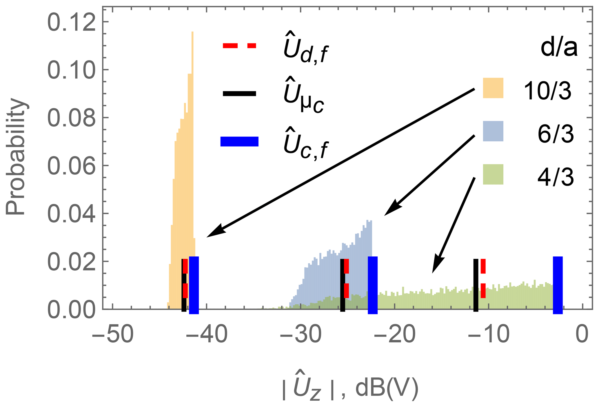
Figure 5 Simulated distributions of the induced voltage $\left|{\widehat{U}}_z\right|$ in a pick-up coil for a circularly modeled 3-D coil with radius a in random orientations at three selected distances d between the 3-D coil and the pick-up coil in an inhomogeneous primary field generated by the exciter wire.

In order to be able to compare the contribution of the two individual effects to the overall voltage variances, the variance coefficient c introduced by Nelson (2012) is chosen as a figure of merit:

$$\begin{array}{}\text{(26)}& c={\displaystyle \frac{\mathit{\sigma }}{\mathit{\mu }}},\end{array}$$

where σ is the empirical standard deviation and μ is the empirical expected value of the corresponding voltage distribution. The independence from absolute values makes the variation coefficient an appropriate figure of merit for our analyses. Using the standard deviation σ alone for the characterization of the uncertainty would make the individual effects shown in Fig. 6 incomparable, since they are based on different primary field strengths.

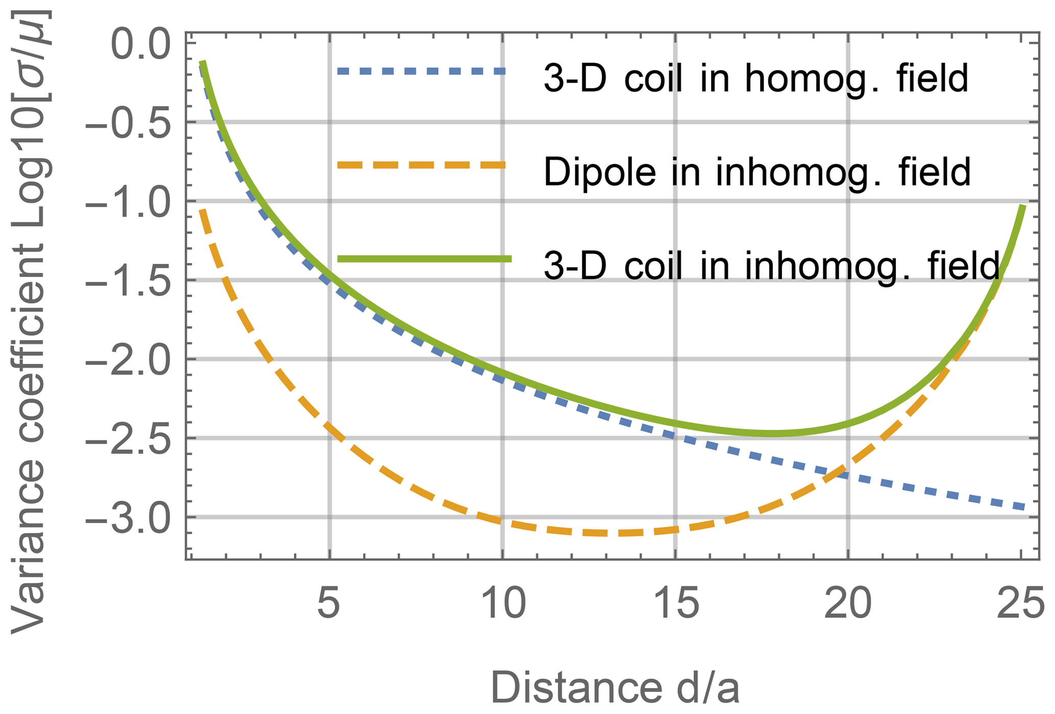
Figure 6 Simulated variance coefficient of the induced voltage $\left|{\widehat{U}}_z\right|$ in a pick-up coil for a randomly oriented 3-D coil and a 3-D dipole over the relative position d∕a in a homogeneous primary field and an inhomogeneous primary field.

In Fig. 6 the logarithmically scaled variance coefficient is shown at each distance d of each of the previously calculated combinations of the primary field and coil model. The distance of the 3-D coil to the pick-up coil is written in a ratio of distance d to coil radius a=0.03 m. At the distances $d/a=\mathrm{0}$ and $d/a=\mathrm{25}$ the exciter wire is positioned. The figure shows an increased effect of the inhomogeneous primary field near the exciter wires as it affects the induced currents in the 3-D coil. With increasing distance to the pick-up coil the effect of the coil geometry decreases as the circular coil field from Eq. (13) converges towards a dipole field as in Eq. (11) with growing distance d∕a. Finally, the combined effect is shown for a circular 3-D coil in an inhomogeneous primary field. Only far from the pick-up coil when the 3-D coil approaches the other side of the shelf, and hence the exciter wire, does the inhomogeneous primary field dominate the variance coefficient c. For values of $d/a<\mathrm{15}$, c is only slightly higher for the 3-D coil in the inhomogeneous primary field than in the homogeneous case.

4 Comparison of localization methods

In this section six localization approaches are introduced, which are later compared by means of simulations and measurements in Sects. 5 and 6, respectively. The goal is to estimate the distance d between a 3-D coil and a pick-up coil based on the measured voltage U₀ induced in the pick-up coil. The primary magnetic field is assumed to be generated by the exciter wire as described in Sect. 2.1 and thus to be inhomogeneous.

The estimators presented in the following can be divided into two categories. Stochastic estimators are built upon the statistical distribution of pick-up coil voltages at each distance d, while table-based estimators only assign a single voltage for each distance.

4.1 Stochastic estimators

Figure 7 shows the probability P(U|d) of the induced pick-up coil voltage $\left|{\widehat{U}}_z\right|$, abbreviated as U in the following, for each relative distance d∕a. This distribution is based on the calculations in Sect. 3.4, where a 3-D coil is positioned in the inhomogeneous primary field of the shelf from Fig. 1. Areas with darker colors in the figure indicate a higher probability of occurrence of a particular voltage U at the corresponding distance d∕a.

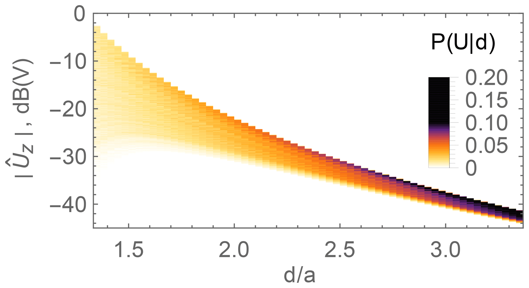
Figure 7 Probability P(U|d) of the pick-up coil voltage $\left|{\widehat{U}}_z\right|$ due to a 3-D coil in an inhomogeneous primary field.

The estimators described in this subsection are based on this distribution, which is computationally very expensive to acquire. For each position (or distance in the 1-D case) a large number N_R of random orientations must be considered to obtain a probability density function of satisfying accuracy. In our case N_R=900 orientations per distance were chosen.

4.1.1 Maximum likelihood estimator

When choosing a fixed voltage U₀, the probability function from Fig. 7 can also be regarded as a likelihood function $L\left(U_{\mathrm{0}}\right|d):=P(U=U_{\mathrm{0}}\left|d\right)$ slicing horizontally through the graph with d as a parameter. The maximum likelihood estimate (MLE) selects that distance ${\widehat{d}}_{\mathrm{MLE}}$ as an estimate, which maximizes the likelihood function L(U₀|d) as described by

$$\begin{array}{}\text{(27)}& {\widehat{d}}_{\mathrm{MLE}}\left(U_{\mathrm{0}}\right)=\underset{d}{\arg max}\left\{L\left(U_{\mathrm{0}}\right|d)\right\}.\end{array}$$

Having exact knowledge of the probability distributions, using an MLE is a common approach. However, if the distributions do not reflect the reality, the MLE will not provide optimal results.

4.1.2 A posteriori mean estimator

Another possible estimator is the a posteriori mean (APM) ${\widehat{d}}_{\mathrm{APM}}$. For that an a posteriori distribution h(d|U₀) has to be derived by means of Bayes' law combining the likelihood function L(U₀|d) with some prior knowledge P(d) about the distribution of d according to

$$\begin{array}{}\text{(28)}& h\left(d\right|U_{\mathrm{0}})={\displaystyle \frac{L\left(U_{\mathrm{0}}\right|d\left)P\right(d)}{{\int }_{-\mathrm{\infty }}^{\mathrm{\infty }}L\left(U_{\mathrm{0}}\right|d^{\prime }\left)P\right(d^{\prime })\mathrm{d}{d}^{\prime }}}.\end{array}$$

The prior knowledge term P(d) can be used to exclude certain unrealistic positions d; e.g., if the space around a specific position is obstructed by obstacles, the localization object cannot be placed there. Also, previous knowledge of the 3-D coil's position can be included in the prior to implement a stochastic filter (e.g., a Kalman filter or a particle filter) tracking the 3-D coil (Simon, 2006). Finally, the APM estimator is the statistical mean of h(d|U₀) obtained by

$$\begin{array}{}\text{(29)}& {\widehat{d}}_{\mathrm{APM}}\left(U_{\mathrm{0}}\right)=\underset{-\mathrm{\infty }}{\overset{\mathrm{\infty }}{\int }}{d}^{\prime }h\left(d^{\prime }\right|U_{\mathrm{0}})\mathrm{d}{d}^{\prime }.\end{array}$$

This estimator is expected to have the smallest mean squared error.

4.1.3 A posteriori median estimator

The third estimator is the median of the a posteriori distribution from Eq. (28). It is obtained by solving the following equation:

$$\begin{array}{}\text{(30)}& h\left(d\right|U_{\mathrm{0}})=\underset{-\mathrm{\infty }}{\overset{{\widehat{d}}_{\mathrm{MED}}}{\int }}h(d\left|U_{\mathrm{0}}\right)\mathrm{d}{d}^{\prime }=\mathrm{0.5}.\end{array}$$

This estimator is expected to have the least absolute error in the estimate. Besides the mean and the median of the a posteriori distribution from Eq. (28), the mode of it forms the maximum a posteriori estimator (MAP). It is neglected here, since for a uniformly distributed a priori probability p(d), as in case of this paper, the MLE and the MAP are identical.

4.2 Table-based estimators

The precomputation of the distributions P(U|d), required for the estimators ${\widehat{d}}_{\mathrm{APM}}$ and ${\widehat{d}}_{\mathrm{MLE}}$, can be avoided by only calculating one single forward solution for the induced voltage in the pick-up coil U_i at each distance d_i. The resulting pairs can be stored in the look-up table described in Sect. 2.2. The table is organized in rows i, each containing a value for d_i and the corresponding theoretical value for the voltage U_i. When localizing, the measured voltage value U₀ can then be compared to all voltage entries U_i in the look-up table. The distance $d_{i^{\prime }}$ in the row i^′ is selected as the estimate $\widehat{d}$, for which the squared difference between the measured voltage U₀ and the table entry $U_{i^{\prime }}$ is smallest:

$$\begin{array}{}\text{(31)}& \widehat{d}\left(U_{\mathrm{0}}\right)=d_i\text{with}i=\underset{i^{\prime }}{\arg min}(U_{i^{\prime }}-U_{\mathrm{0}}{)}^{\mathrm{2}}.\end{array}$$

In the precomputation phase only one instead of N_R model evaluations is required, obviously reducing time complexity by a factor of N_R at the same distance resolution.

For practical setups with more than one pick-up coil a suitable metric needs to be selected for the comparison operation. A simple choice is the sum of the squared differences, i.e., the square of the Euclidean distance. However, as the induced voltage in the pick-up coils is a highly nonlinear function of the 3-D coil's position, the Euclidean distance is often a suboptimal choice. It tends to put the highest weight on the largest pick-up coil voltages, which unfortunately are the ones with the largest coefficients of variation, as shown in Sect. 3. Investigation of that topic is reserved for future work.

In the following several possibilities for the forward solution U_i are described.

4.2.1 Fixed-orientation dipole model

A simple approach to a forward solution for U_i is based on the dipole model (Eq. 11). For each distance d_i the corresponding induced voltage $U_i={\widehat{U}}_{\mathrm{d},\mathrm{f}}$ is calculated via the dipole model with fixed orientation in the z direction, as also described in Sect. 3.4 and shown in Fig. 5. We call the corresponding distance estimate ${\widehat{d}}_{\mathrm{d},\mathrm{f}}$. The advantages of this model are its simplicity and therefore small calculation time.

4.2.2 Fixed-orientation coil model

A second possible forward solution approach is to calculate the induced voltage $U_i={\widehat{U}}_{\mathrm{c},\mathrm{f}}$ from a circular 3-D coil with a fixed orientation in the z direction, as also shown in Fig. 5. We call the corresponding distance estimate ${\widehat{d}}_{\mathrm{c},\mathrm{f}}$. This approach is slightly more expensive in terms of calculation time as we need to use the model described in Sect. 3.2 for the magnetic field of a circular loop instead of the closed-form dipole model.

4.2.3 Mean voltage coil model

Accepting a higher computational effort, we can also calculate the induced voltages for many different orientations of the 3-D coil for each position d_i and take the mean of the attained voltage distribution. This corresponds to using U_i=μ_c from Fig. 5 for each table entry. We call the corresponding distance estimate ${\widehat{d}}_{{\mathit{\mu }}_{\mathrm{c}}}$.

5 Simulation of the localization error

In the following the localization errors of the six methods described in Sect. 4 are simulated and compared. As before, for reasons of simplicity, we only consider localization in one dimension here. As the primary magnetic field source, the exciter wire around our shelf as described in Sect. 2.1 is used again. We select the simulated positions d_t along a linear trajectory in the x–y plane running from the middle of a pick-up coil perpendicular to the exciter wire at that point towards the inside of the shelf. In this case, because of the symmetry of the shelf setup, all pick-up coils behave the same. Hence, the selection of a specific one can be done arbitrarily. The step size between the individual positions d_t is set to 1 mm. For the statistical analysis, m=100 orientations are randomly selected at each position d_t. At each orientation of the 3-D coil the induced voltage in the pick-up coil is calculated and Gaussian noise with a standard deviation of 325 nV is added. This is the noise level we see in our practical shelf setup. The mapping of the noisy calculated voltages U_calc to the estimated distances $\widehat{d}$ is done with each localization method described in Sect. 4 according to Eqs. (27), (29), (30) and (31). For the APM estimator a uniform prior knowledge of P(d) is used. At each actual position d_t the mean absolute error err(d_t) of the particular localizers' estimates is calculated as

$$\begin{array}{}\text{(32)}& \mathrm{err}\left(d_t\right)={\displaystyle \frac{\mathrm{1}}{m}}\sum _{n=\mathrm{1}}^m\mathrm{|}{\widehat{d}}_{t,n}-d_t\mathrm{|}.\end{array}$$

The results of the simulation are shown in Fig. 8 and are zoomed in for small distances d in Fig. 9. It can be observed that at positions of the 3-D coil close to the pick-up coil, the estimators ${\widehat{d}}_{{\mathit{\mu }}_{\mathrm{c}}}$, ${\widehat{d}}_{\mathrm{d},\mathrm{f}}$, ${\widehat{d}}_{\mathrm{MED}}$ and ${\widehat{d}}_{\mathrm{APM}}$ provide smaller localization errors than the ${\widehat{d}}_{\mathrm{MLE}}$ and ${\widehat{d}}_{\mathrm{c},\mathrm{f}}$ estimators. At relative distances of approximately $d/a=\mathrm{15}$ and more the estimators generate similar localization errors. At these distances the simulated noise in the pick-up coil voltage starts to be the dominant contributor to the estimation error. The influence of the primary field's inhomogeneity as well as the geometrical extent of the 3-D coil become negligible.

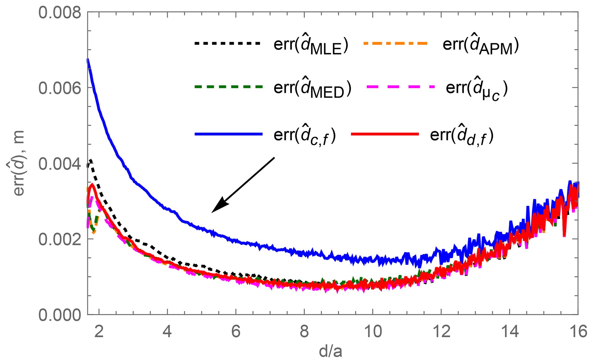
Figure 8 Simulated mean localization error at different positions d of six localization methods.

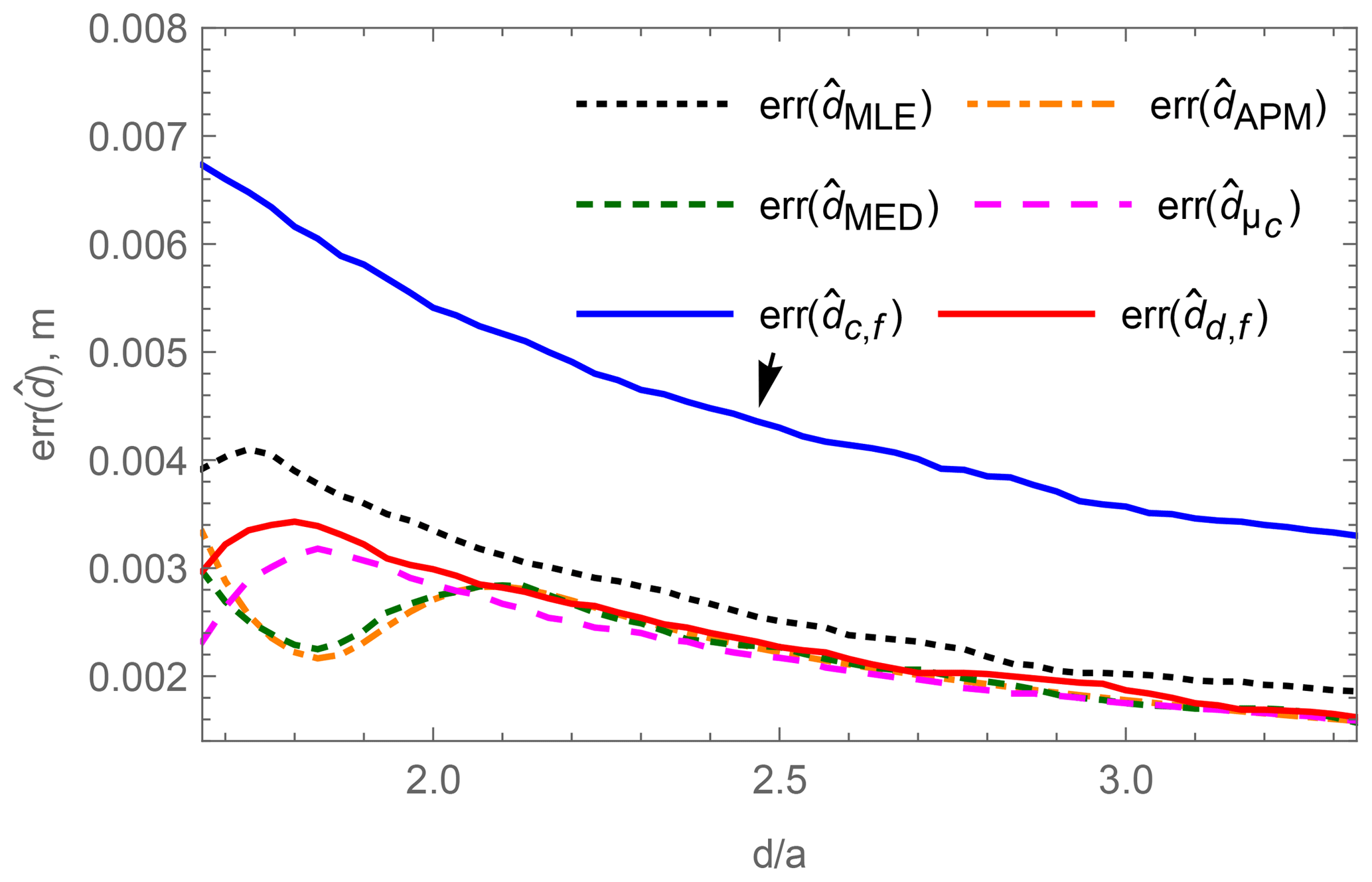
Figure 9 Simulated mean localization error at different positions d of six localization methods for small relative distances d∕a.

Especially in Fig. 9 the estimation errors around the relative distances $d/a=\mathrm{1.7}$ show contradictory tendencies. The table-based methods ${\widehat{d}}_{{\mathit{\mu }}_{\mathrm{c}}}$, ${\widehat{d}}_{\mathrm{d},\mathrm{f}}$ as well as ${\widehat{d}}_{\mathrm{MLE}}$ start with a lower localization error which first rises with increasing distances d but then falls again, whereas ${\widehat{d}}_{\mathrm{MED}}$ and ${\widehat{d}}_{\mathrm{APM}}$ have a valley of decreasing error around a relative distance of $d/a=\mathrm{1.85}$.

The explanation of those effects can be found when looking at the individual estimators' mapping functions of measured voltages $\left|{\widehat{U}}_Z\right|$ to estimated distances $\widehat{d}$. In Fig. 10 the mapping of the stochastic estimators and in Fig. 11 the mapping of the table-based estimators are shown. In both figures the probability distribution P(U|d) of the voltage $\left|{\widehat{U}}_z\right|$ at a given distance d is overlaid.

Except for the ${\widehat{d}}_{\mathrm{APM}}$ estimator, which has a continuous mapping, the estimators map ranges of voltages to distinct distances in the previously calculated 1 mm grid. The voltage ranges of the estimators at a particular distance provide an indication of the expected localization error. The broader the voltage range, the lower the position estimation error at that particular distance. However, that comes with the cost of a less broad voltage range, and therefore with a higher localization error, at other distances. Not only the voltage range at the particular distance influences the localization error, but also the position and the steepness of the mapping function. As can be seen in Fig. 11, the ${\widehat{d}}_{\mathrm{c},\mathrm{f}}$ estimator provides a biased estimate. The influence of the steepness can be seen between the ${\widehat{d}}_{\mathrm{MED}}$ and the ${\widehat{d}}_{\mathrm{MLE}}$ estimator: although the ${\widehat{d}}_{\mathrm{MLE}}$ estimator has a broader voltage range at the lowest distance, its mapping function is steeper and therefore its localization error is higher than the one from the ${\widehat{d}}_{\mathrm{MED}}$ estimator.

Figure 10 Mapping of the measured voltage $\left|{\widehat{U}}_Z\right|$ to the estimated distance $\widehat{d}$ for the stochastic estimators ${\widehat{d}}_{\mathrm{APM}}$, ${\widehat{d}}_{\mathrm{MED}}$ and ${\widehat{d}}_{\mathrm{MLE}}$ overlaid with the normalized voltage probability distribution P(U|d) at any given distance d.

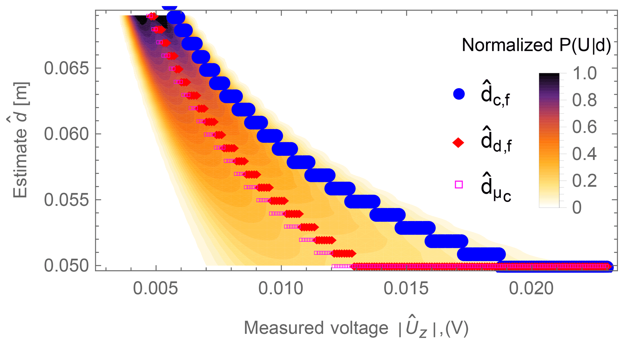
Figure 11 Mapping of the measured voltage $\left|{\widehat{U}}_Z\right|$ to the estimated distance $\widehat{d}$ for the table-based estimators ${\widehat{d}}_{\mathrm{c},\mathrm{f}}$, ${\widehat{d}}_{\mathrm{d},\mathrm{f}}$ and ${\widehat{d}}_{{\mathit{\mu }}_{\mathrm{c}}}$ overlaid with the normalized voltage probability distribution P(U|d) at any given distance d.

6 Measurements

In order to verify the theoretical distribution of the induced voltage, a measurement has been conducted on the setup defined in Sect. 5. A 3-D coil has been positioned at different distances d in the x direction from the upper-left z-oriented pick-up coil along the pick-up coil's center line. At each distance d the 3-D coil has been rotated arbitrarily 20 times and the corresponding induced voltage in the pick-up coil has been measured. Based on the measurements, the variation coefficient, as defined in Eq. (26), has been calculated and is compared to a simulated variation coefficient in Fig. 12. One simulation is made without noise and the other is calculated with an additive Gaussian noise of 325 nV, which has been measured in the reader. As expected, the measured voltage variation decreases with the distance d but increases slightly from a distance of approximately $d/a=\mathrm{20}$ again due to the inhomogeneity of the primary field due to the opposite exciter wire. In the middle of the shelf the variation coefficient based on the measured voltages shows a constant plateau which is induced by the dominating effect of the Gaussian noise and positioning errors of the manually conducted measurements. At the normalized distance between $d/a=\mathrm{12}$ and $d/a=\mathrm{14}$ no measurements could be taken, since a shelf plank was in the way.

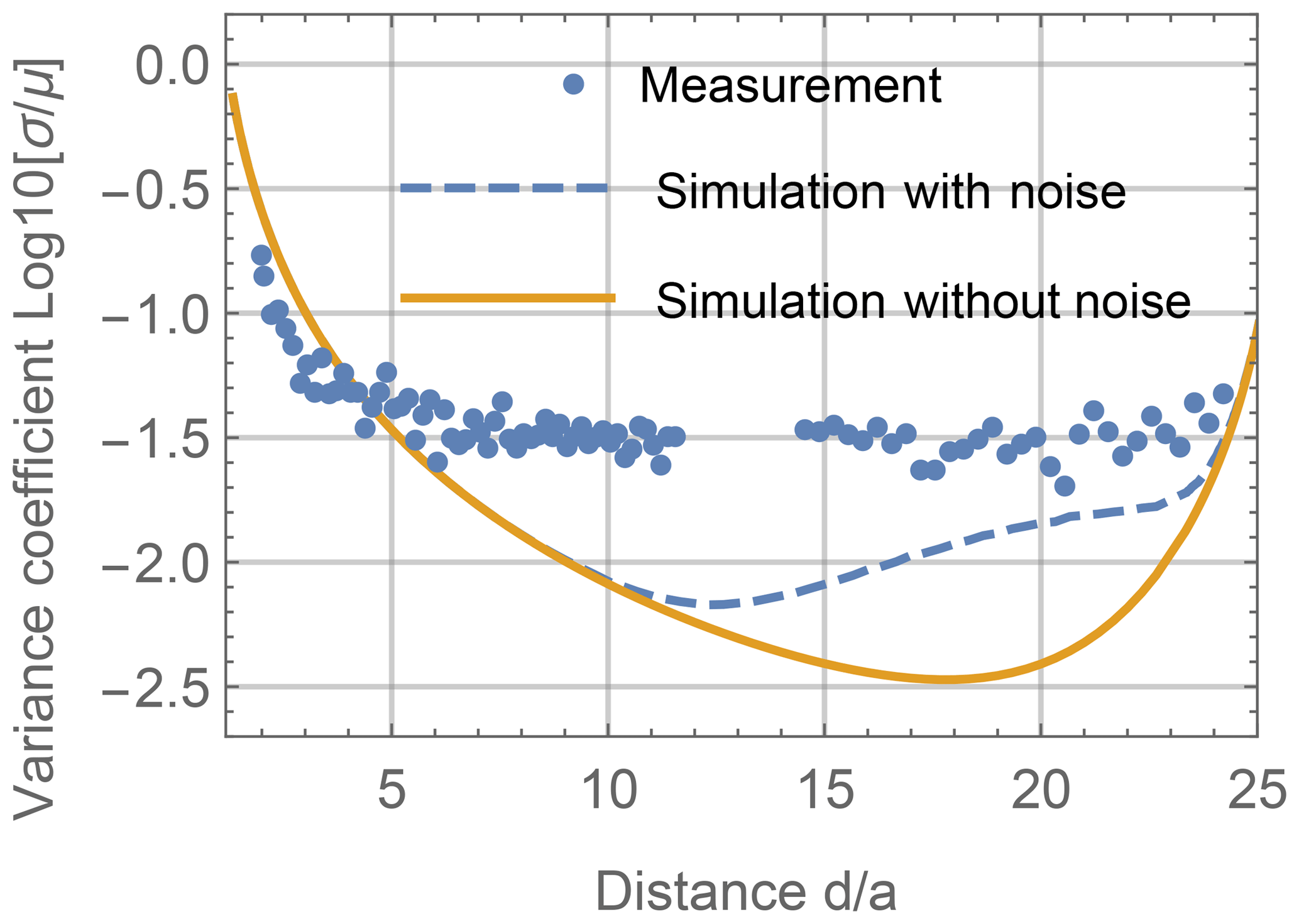
Figure 12 Measured logarithmic variation coefficient c of induced voltage ${\widehat{U}}_z$ in a pick-up coil for an arbitrarily oriented 3-D coil at different positions d.

In a second analysis the estimators defined in Sect. 4 have been applied to the measurement data. For each estimator the localization error has been calculated and is shown in Fig. 13. Comparing Fig. 13 with the simulated localization error in Fig. 8 shows that close to the pick-up coil all estimators perform worse and the localization errors decrease with increasing distance d. From a relative distance of $d/a=\mathrm{6}$ in the measurement and a relative distance $d/a=\mathrm{10}$ in the simulation, the localization errors increase due to noise. Positions farther than $d/a=\mathrm{16}$ are not analyzed since ambiguity arises due to the increasing measured voltage closer to the opposite exciter wire. Measurements show that close to the pick-up coil the estimator based on the 3-D coil with fixed orientation ${\widehat{d}}_{\mathrm{c},\mathrm{f}}$ from Sect. 4.2.2 shows the highest error and the maximum likelihood estimator ${\widehat{d}}_{\mathrm{MLE}}$ from Eq. (27) shows the second worst performance, which is in accordance with the simulation results in Fig. 9. The remaining estimators show similar results. At positions farther than $d/a=\mathrm{7}$, where the Gaussian noise and the positioning error of the measurement setup are dominant, all estimators show equal behavior.

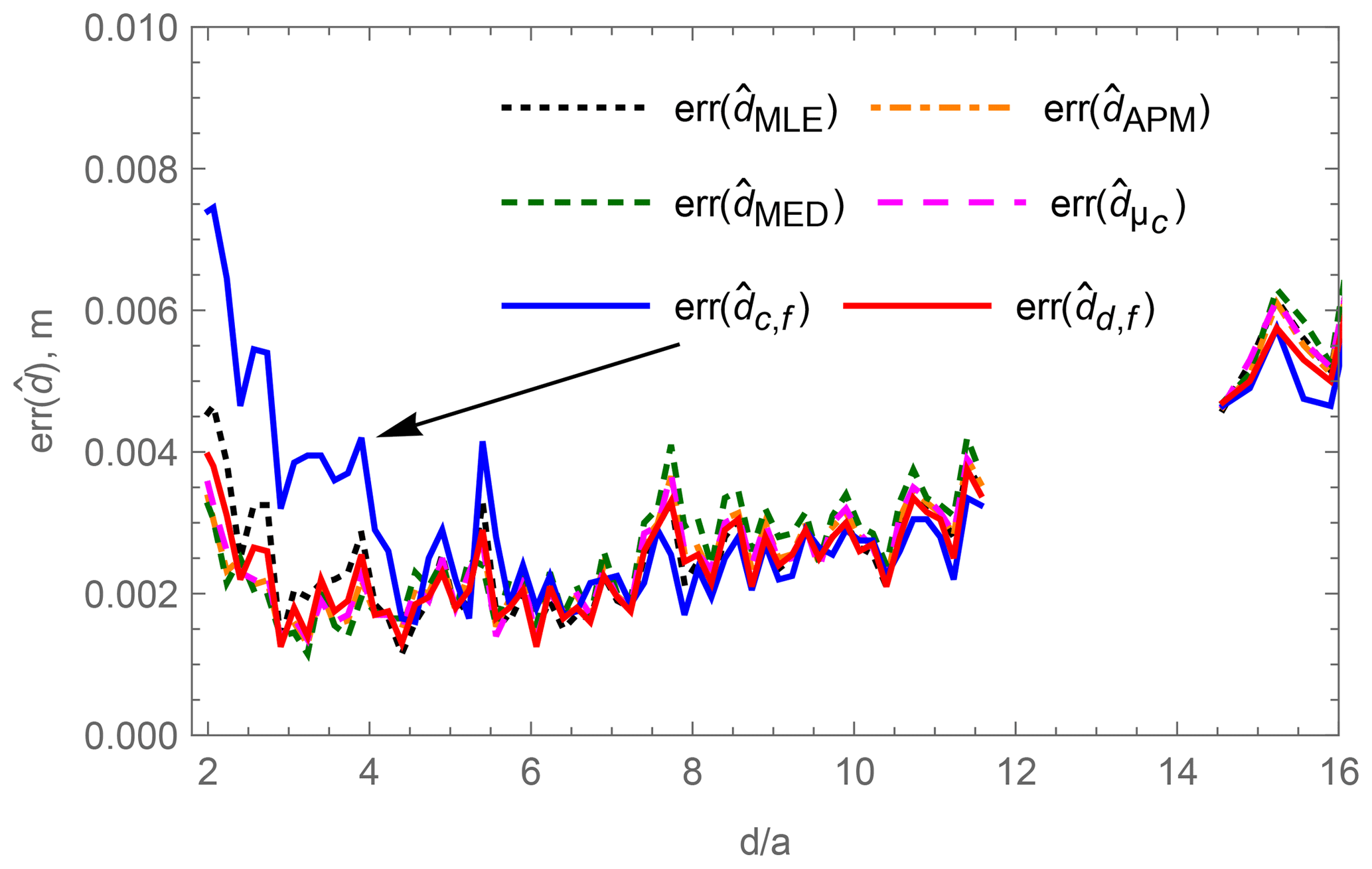
Figure 13 Measured mean localization error at different positions d of five localization methods.

7 Discussion

The simulation and measurement results show that for the position estimation in the 1-D case only positions close to the pick-up coil are sensitive to the selection of a certain estimator. Further away from the pick-up coil noise is the dominant influence on the localization error and equally influences all estimators. Close to the pick-up coil the maximum likelihood estimator ${\widehat{d}}_{\mathrm{MLE}}$ and the estimator based on the forward model with the fixed coil position ${\widehat{d}}_{\mathrm{c},\mathrm{f}}$ are not recommended. Throughout the analyzed region the a posteriori mean estimator ${\widehat{d}}_{\mathrm{APM}}$, the a posteriori median estimator ${\widehat{d}}_{\mathrm{MED}}$, the estimator based on the fixed oriented dipole model ${\widehat{d}}_{\mathrm{d},\mathrm{f}}$ and the estimator based on the mean voltage of the arbitrarily rotated 3-D coil ${\widehat{d}}_{{\mathit{\mu }}_{\mathrm{c}}}$ show equally low localization errors. However, from those four estimators the fixed oriented dipole model has the least computational effort due to the simple model and is therefore recommended.

Using more distributed pick-up coils and extending the 1-D localization to a 2-D or 3-D localization may have influence on the performance of the individual estimators. In contrast to the other estimators the stochastic estimators can include a priori knowledge, like not accessible positions due to the geometry of the shelf or due to the last known position combined with a movement model of the localization object. A weighting of the pick-up coil signals based on the signal-to-noise ratio may also be applied in the future.

The differences between the simulation and the measurements arise from the sensitive manual measurement setup, where the exact positioning of the 3-D coil is difficult. A big influence on the results may arise from different electrical and geometrical characteristics of the 3-D coils. In the simulations geometrically and electrically identical coils were assumed. However, in reality different coil areas, different qualities of the resonance as well as the exact resonance frequency itself have a huge influence on the amplitude of the secondary field strength of each of the three coils of the 3-D coil. On the one hand using high quality for the resonant circuit of the coil provides a higher current and hence a stronger secondary field. On the other hand a high-quality resonant circuit is very sensitive to the surrounding and may be detuned easily. A detuning of the resonance frequency leads to a drop in the field strength of that coil. It is assumed that this effect has a big influence on the localization accuracy and will therefore be investigated in the future.

8 Conclusion

In this paper the uncertainty of the field distribution from an arbitrarily oriented 3-D coil in a primary magnetic field is investigated analytically. The sensitivity of the field distribution against two effects, the inhomogeneity of the primary field and the geometrical extent of the 3-D coil, is presented. Three stochastic and three non-stochastic position estimators are proposed. Their theoretical absolute mean estimation errors are compared by simulations. Finally measurements on a laboratory setup for inductive localization are conducted to verify the field variation as well as the localization errors of the individual estimators. It is shown that from a certain distance between the field sensor and the 3-D coil, the effects of the field distribution on the localization error can be neglected. Future work will comprise analyses of the influence of the characteristics of the individual coils from the 3-D coil on the field distribution as well as the influence of the geometrical extent of the field sensors.

Appendix A: Generation of random orientations

For an uncertainty analysis of the rotation effect on the induced voltages in the system's pick-up coils, arbitrary orientations of the 3-D coil have to be calculated. It is convenient to regard the two rotation angles Ψ and Θ as azimuth angle ϕ and zenith angle θ of the spherical coordinates with the defined ranges of $\mathrm{0}\le \mathit{\varphi }<\mathrm{2}\mathit{\pi }$ and $\mathrm{0}\le \mathit{\theta }<\mathit{\pi }$, respectively. In order to get equally distributed arbitrary orientations, one can think of equally distributed points on the surface of a unit sphere, based on variations of the two spherical angular coordinates ϕ and θ. The third rotation angle Φ can then be uniformly distributed between 0 and 2π. Selecting the two spherical angles from a uniform distribution results in an aggregation of surface points at the poles of the sphere around the z axis (Weisstein, 2018). Therefore a combination of methods described in Marsiagla (1972) and Arvo (1992) is applied to receive arbitrary orientations. Thereby firstly a set of random points

$$\begin{array}{}\text{(A1)}& {\mathit{P}}_{\mathrm{C}}=\left\{(x_j,y_j,z_j{)}^{\mathrm{T}}|j=\mathrm{1}\mathrm{\dots }N\right\}\subseteq {\left[-\mathrm{1},\mathrm{1}\right]}^{\mathrm{3}}\end{array}$$

from a uniform distribution within the volume of a cube is generated. The values of x, y and z lie within the interval of $\left[-\mathrm{1};\mathrm{1}\right]$ each. From that set of points those are selected that lie within the volume of a unit sphere and are further projected onto the sphere's surface by

$$\begin{array}{ll}{\displaystyle }& {\displaystyle }{\mathit{P}}_{\mathrm{sph}}=\left\{{\displaystyle \frac{(x,y,z{)}^{\mathrm{T}}}{d}}\left|\right(x,y,z{)}^{\mathrm{T}}\in {\mathit{P}}_{\mathrm{C}}\right.\\ \text{(A2)}& {\displaystyle }& {\displaystyle }\left.\text{with}d=\sqrt{x^{\mathrm{2}}+y^{\mathrm{2}}+z^{\mathrm{2}}}<\mathrm{1}\right\}.\end{array}$$

The resulting set of Cartesian position vectors P_sph is equally distributed on the sphere surface. Those points can be transformed into spherical coordinates θ and ϕ by

$$\begin{array}{}\text{(A3)}& {\displaystyle }& {\displaystyle }\mathit{\theta }=\arctan {\displaystyle \frac{y}{x}},\text{(A4)}& {\displaystyle }& {\displaystyle }\mathit{\varphi }={\displaystyle \frac{\mathit{\pi }}{\mathrm{2}}}-\arccos z,\end{array}$$

and can be interpreted further as the rotation angles Ψ and Θ. The third arbitrary rotation angle Φ can be selected uniformly randomly in the interval [0;2π].