Deep neural networks for computational optical form measurements

Deep neural networks have been successfully applied in many different fields like computational imaging, healthcare, signal processing, or autonomous driving. In a proof-of-principle study, we demonstrate that computational optical form measurement can also benefit from deep learning. A data-driven machine-learning approach is explored to solve an inverse problem in the accurate measurement of optical surfaces. The approach is developed and tested using virtual measurements with a known ground truth.

1 Introduction

Deep neural networks and machine learning, in general, are experiencing an ever greater impact on science and industry. Their application has proven beneficial in many different domains, including autonomous driving (Grigorescu et al., 2020), anomaly detection in quality management (Staar et al., 2019), signal processing (Mousavi and Baraniuk, 2017), analysis of raw sensor data (Moraru et al., 2010), or healthcare (Esteva et al., 2019; Kretz et al., 2020). Machine-learning methods have also been successfully employed in optics. Examples comprise the compensation of lens distortions (Chung, 2018) or correcting aberrated wave fronts in adaptive optics (Vdovin, 1995). Furthermore, machine learning has been used for misalignment corrections (Baer et al., 2013; Zhang et al., 2020), aberration detection (Yan et al., 2018), or phase predictions (Rivenson et al., 2018).

Deep learning techniques became very popular, especially for computational imaging applications (Barbastathis et al., 2019), with the introduction of convolutional networks (LeCun et al., 2015). But, to the best of our knowledge, deep learning has not yet been applied for the accurate computational measurement of optical aspheres and freeform surfaces in predicting the surface under test from its optical path length differences. The precise reconstruction of aspheres and freeform surfaces is currently limited by the accuracy of optical form measurements, with an uncertainty range of approximately 50 nm (Schachtschneider et al., 2018). The aim of this paper is to demonstrate, through a proof-of-principle study, that this field in optics can also significantly benefit from machine-learning techniques.

Our investigations were conducted using the SimOptDevice (Schachtschneider et al., 2019) simulation toolbox. The toolbox provides realistic, virtual experiments with a known ground truth. We concentrated on the tilted-wave interferometer (TWI) (Baer et al., 2014) for the experimental realization. It is a promising technique for the accurate computational measurement of optical aspheres and freeform surfaces, using contact-free interferometric measurements. The TWI combines a special measurement setup with model-based evaluation procedures. Four charge-coupled device (CCD) images with several interferograms are generated by using multiple light sources to illuminate the surface under test. A simplified scheme is shown in Fig. 1. See Garbusi et al. (2008) for more detailed explanations. The test topography is then reconstructed by solving a numerically expensive nonlinear inverse problem by comparing the measured optical path length differences to simulated ones, using a computer model and the known design of the surface under test. In this study, Physikalisch-Technische Bundesanstalt's realization of the TWI evaluation procedure is considered (Fortmeier et al., 2017).

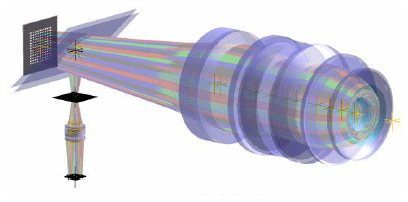
Figure 1 Schematic of the tilted-wave interferometer (reference arm not shown). The 2D point source array is on the left, the specimen is on the right, and the CCD is at the bottom.

While the great success of deep networks is based on their ability to learn complex relations from data without knowing the underlying physical laws, including existing physical knowledge into the models can further improve the results (see de Bézenac et al., 2019; Karpatne et al., 2017; Raissi, 2018). In our study, we also follow such an approach by developing a hybrid method which combines physical knowledge with data-driven deep neural networks. The employed scientific knowledge is twofold; training data are generated by physical simulations, and a conventional calibration method is used to generalize the trained network to nonperfect systems.

This paper is organized as follows. Section 2 briefly introduces neural networks and presents the proposed deep learning framework. The means of generating the training data and the details of training the network are explained, combining this approach with a conventional calibration method for better generalization. The results obtained for the independent test data are then presented and discussed in Sect. 3. Finally, some conclusions are drawn from our findings, and possible future research is suggested.

2 Hybrid method

This section provides an overview of deep neural networks and introduces the hybrid method that was developed, which combines the TWI procedure with a data-driven deep learning approach. Without a loss of generality, each specimen can be assumed to have a known design topography. The overall goal of form measurement is to determine the deviation ΔT of a specimen T_s to the given design topography T_d, i.e., $T_{\mathrm{s}}=T_{\mathrm{d}}+\mathrm{\Delta }T$. To this end, the TWI provides measurements of the optical path length differences L_s of the specimen being tested. Simultaneously, a computer model (Schachtschneider et al., 2019) computes the optical path length differences L of a given topography T. The inverse problem is to reconstruct the specimen topography $T_{\mathrm{s}}=T_{\mathrm{d}}+\mathrm{\Delta }T$ from its measured optical path length differences L_s.

The conventional evaluation procedure of the TWI is numerically expensive and relies on linearization. A general advantage of neural networks is their ability to produce instant results once they are trained. Furthermore, it is interesting to explore whether deep learning could also improve the quality of the inverse reconstruction as a nonlinear approach. We aim to address the inverse problem described above using deep networks, i.e., by reconstructing a difference topography ΔT from given differences of optical path length differences $\mathrm{\Delta }L=L_{\mathrm{s}}-L_{\mathrm{d}}$.

2.1 Data generation

When solving an inverse problem with neural networks, it is common practice to generate data through physical simulations (Lucas et al., 2018; McCann et al., 2017). Here, various difference topographies ΔT are generated through randomly chosen, weighted Zernike polynomials. They are then added to a specific design topography at a fixed measurement position to create different virtual specimens. The sequence of Zernike polynomials yields an orthogonal basis of the unit disc and is a popular tool in optics for modeling wave fronts (Wang and Silva, 1980). Following the forward pass, the computer model is used to compute the optical path length differences of the design topography and the modeled specimens. Note that the data are generated assuming perfect system conditions, i.e., the computer model is undisturbed. An example can be seen in Figs. 3 and 4.

Data were generated for two different design topographies, with about 22 000 data points for each design. It should be noted that 10 % of the data was used exclusively for testing and was not included in the network training.

2.2 Deep neural network architecture

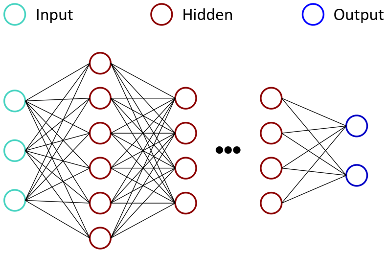
A simple, fully connected neural network with a single hidden layer is represented by a nonlinear function $f_{\mathrm{\Phi }}:\mathbb{R}\to \mathbb{R}$, with parameters $\mathrm{\Phi }=\left\{{\mathit{\omega }}_i,b_i\in \mathbb{R}|i=\mathrm{1},\mathrm{\dots },n\right\}$, where n is the number of neurons in the hidden layer. The univariate output of the network is modeled as $f_{\mathrm{\Phi }}\left(x\right)={\sum }_{i=\mathrm{1}}^n\mathit{\sigma }({\mathit{\omega }}_{i}x+b_i)$, x∈ℝ, where σ is a nonlinear activation function. In general, input and output have high dimensions, and the architecture can become arbitrarily deep by adding more layers. Neural networks with high complexity are called deep neural networks. An example of this type of architecture is shown in Fig. 2. There, two outputs are predicted based on three given inputs after processing the information through several hidden layers. Also, different types of layers – convolutional layers (LeCun et al., 2015), for example – can be used instead of fully connected ones. The network parameters can be optimized, via backpropagation on the given training data, by minimizing a chosen loss function between the predicted and known output.

Figure 2 An example of deep neural network architecture.

At this point, it is important to consider the network as being an image-to-image regression function f_Φ which maps the differences of optical path length differences ΔL (see Fig. 4) onto a difference topography ΔT (see Fig. 3); i.e., $f_{\mathrm{\Phi }}:{\mathbb{R}}^{M\times M\times K}\to {\mathbb{R}}^{M\times M}$, ΔL↦ΔT, where Φ are the network parameters to be trained, M×M is the dimension of the images, and K is the number of channels in the input. Note that the image dimension of the input equals the image dimension of the output here. This is not mandatory, but it suits the network architecture described below very well. While the CCD gives a resolution of 2048×2048 pixels, we chose M=64. For the asphere and the multispherical freeform artifact (Fortmeier et al., 2019), as seen in Fig. 4, K=4 and K=1 were used, respectively. This is because the multispherical freeform artifact has a big patch in the first channel, which almost covers the entire CCD for the selected measurement position. Furthermore, even though some pixels are missing, the first channel sufficed for the purpose of this deep learning proof-of-principle study.

Figure 3 An example of difference topography ΔT on a 64×64 pixel grid.

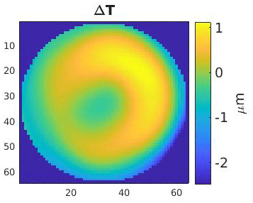
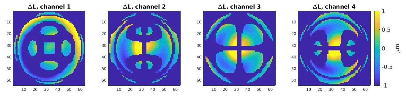
Figure 4 An example of the calculated differences of optical path length differences for one specimen ΔL, with an asphere as the underlying design topography. The four different images originated from the disjointed sets of wave fronts that resulted from the four different mask settings at the 2D point source array.

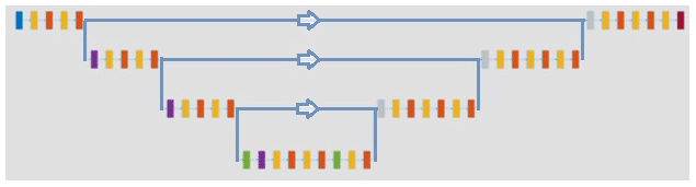
We chose a U-Net as the network architecture. U-Nets have been successfully applied in various image-to-image deep learning applications (Işıl et al., 2019). An example of its structure is shown in Fig. 5. The input passes through several convolution and rectified linear unit layers on the left side before being reduced in dimension in every vertical connection. After reaching its bottleneck at the bottom, the original data dimension is restored, step by step, through transposed convolution layers on the right side. During each dimensional increase step, a depth concatenation layer is added, which links the data of the current layer to the data of the former layer with same dimension. These skip connections are depicted as horizontal lines in Fig. 5.

Figure 5 An example of a U-Net structure.

Here, the chosen U-Net architecture consists of a total of 69 layers. The training set was used to normalize all input and output data prior to feeding them into the network. The U-Net was trained using an Adam optimizer (Kingma and Ba, 2014) and the mean squared error as the loss function. About 2 h of training was carried out for the multispherical freeform artifact, with an initial learning rate of 0.0005, a drop factor of 0.75 every five periods, and a mini batch size of 64. In addition, a dual norm regularization of the network parameters with a regularization parameter of 0.004 was employed to stabilize the training. For the asphere, training was carried out for 15 epochs, with a mini batch size of eight samples, an initial learning rate of 0.0005, which decreased every 3 epochs by a learning rate drop factor of 0.5, and a regularization parameter of 0.0005.

2.3 Generalization to nonperfect systems

In real world applications no perfect systems exist. Thus, the computer model needs to be adapted phenomenologically. In the conventional calibration procedure, the beam path is calibrated through the computer model by using known, well-fabricated spherical topographies at different measurement positions to compare the optical path length differences measured by the TWI and its computer model (Fortmeier, 2016).

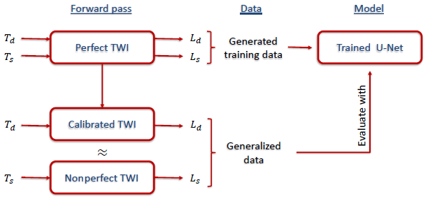
It is not feasible to generate an entirely new database and train a new network after each system calibration when using deep networks. Nonetheless, the ultimate goal is to apply the trained deep network to real world data. To this end, we propose a hybrid method that trains the selected U-Net on data generated under perfect system conditions but also generalizes well to nonperfect systems by evaluating data derived through the conventional calibration method. A workflow chart of the hybrid method is shown in Fig. 6.

Figure 6 Workflow of the developed hybrid method.

3 Results

The following results are all based on simulated data. As mentioned above, two different design topographies are considered, namely an asphere and a multispherical freeform artifact. First, the results of the data acquired from a perfect system environment are presented. The networks which were trained for the design topography of an asphere and a multispherical freeform artifact are addressed, respectively. Next, additional strategies, which could improve the models, are discussed as well. Finally, the application of the hybrid method which was developed is presented in a nonperfect system environment.

The presented results are reproducible in the sense that, when repeating the simulations for similar train and test sets, essentially the same findings are observed. The topographies have a circle as in the base area. Since the required input and output of the network are images, the area outside of the circular shape is defined with zeros, which the network learns to predict. Nonetheless, only the difference topography pixels inside the circular shape are considered in the presented results.

3.1 Perfect system

About 2200 samples were used for testing. They were not included in the training. First, the multispherical freeform artifact was considered as the design topography. Three randomly chosen prediction examples are shown in Fig. 7. The root mean squared error of the U-Net predictions on the test set is 33 nm. For comparison, the difference topographies in the test set have a total root mean squared deviation of 559 nm. The median of the absolute errors of the U-Net is about 18 nm, while the median of total absolute deviations in the test set is 428 nm.

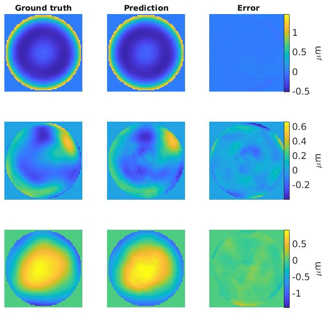
Figure 7 Three examples of predicted test difference topographies. The errors in the third column show the differences between the ground truth and the prediction. The root mean squared errors, from top to bottom, are 16, 84, and 74 nm.

For the asphere as the design topography, the root mean squared error is 102 nm, while the test set has a root mean squared deviation of 589 nm. The median of the absolute errors of the U-Net is 52 nm, and the median absolute deviation of the test set is 451 nm, for comparison. One possible explanation for the discrepancy in the accuracy of the predictions between the network for the asphere and multispherical freeform artifact as the design topographies is the following. The input of the respective U-Nets and their resulting architecture varies widely. As mentioned above, the network concerning the asphere has four input channels. These can be seen in Fig. 4. In each channel, various different areas are illuminated at the CCD, resulting in a distribution of information into different and smaller patches. The multispherical freeform artifact, on the other side, illuminates one big circular shaped patch in the first channel for the selected measurement position. This channel, which contains most of the important information in a single patch, forms the only input to the corresponding network.

However, the results for the asphere can be improved further. One way to do so is to increase the amount of training data (see Fig. 8). As the input has four channels for the asphere, it seems natural that more data are needed for training than for the multispherical freeform artifact. A second approach is to use a network ensemble (Zhou, 2009) rather than a single trained network. To this end, 15 U-Nets were trained from scratch, and the ensemble output was taken as the mean of the ensemble predictions. The results are shown in Fig. 8. In this way, the accuracy was already improved to a root mean squared error of 80 nm, using an ensemble of 15 U-Nets each trained from scratch on almost 28 000 data points. It should be noted that a further improvement seems possible as the amount of data is crucial for training, and the network's architecture of the asphere is more complex due to more input channels.

Figure 8 Root mean squared error (RMSE) of a single network (blue) and a network ensemble (red), depending on the amount of data used for training. The test set is the same for all evaluations and was not included in training.

3.2 Nonperfect system

In any real world application, no experiment is carried out under perfect system conditions. This motivated the idea of disturbing the perfect simulated forward pass and of generalizing the model to nonperfect systems. The network now needed to cope with data coming from a nonperfect TWI after having trained on a perfect simulation environment in the first stage. This was achieved by using a conventional calibration to determine the correct model of the interferometer.

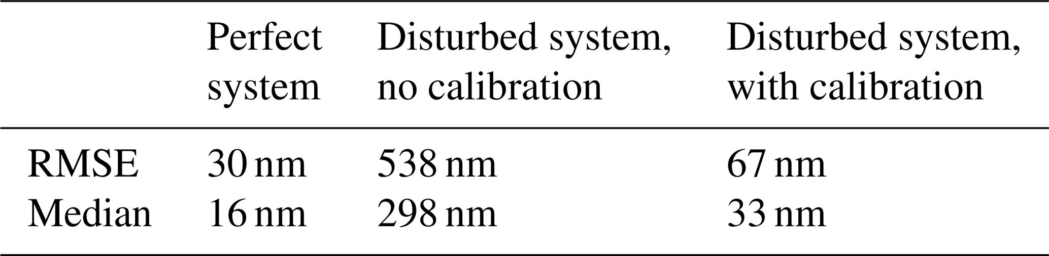
Here, we focused on the multispherical freeform artifact as the design topography. A total of 30 difference topographies were randomly chosen from the former test set, i.e., not included in U-Net training. They had a total root mean squared deviation of 545 nm and ranged from 296 nm to 6.1 µm in their absolute maximal deviation from peak to valley. The results are shown in Table 1, where the same trained network was used for differently produced inputs. The root mean squared error of the network predictions was 30 nm on the perfect TWI system. This increased to 538 nm after having disturbed the TWI system. The trained network is incapable of predicting properly. However, the error can be reduced to 67 nm by using a calibrated forward pass to produce the input data. Hence, our proposed hybrid method can also generalize to nonperfect systems.

Table 1 Root mean squared error and the median of absolute errors for the predictions of the same U-Net using different inputs. The perfect TWI system, which was also used to generate the training data, is in the first column, the disturbed TWI system without calibration is in the second column, and the hybrid method is in the third column.

4 Conclusions

The obtained results are promising and suggest that deep learning can be successfully applied in the context of computational optical form measurements. The presented results are based on simulated data only, and they constitute a proof-of-principle study rather than a final method that is ready for application. An extensive comparison with conventional methods is the next step. Testing the approach on real measurements and accounting for fine-tuning (such as the calibration of the numerical model of the experiment) is reserved for future work as well. Nevertheless, these initial results are encouraging, and once trained, a neural network solves the inverse problem with orders of magnitude faster than the currently applied conventional methods. We conclude from our findings that computational optical form metrology can also greatly benefit from deep learning.