the Creative Commons Attribution 4.0 License.
the Creative Commons Attribution 4.0 License.
 | 08 Oct 2020
A tactile sensor based on magneto-sensitive elastomer to determine the position of an indentation
Simon Gast
Klaus Zimmermann
In this paper, we investigate the capabilities of a tactile sensor based on magneto-sensitive elastomers (MSEs). The main feature of the sensor is the determination of the position of indentation. The principle is based on inductance measurements of multiple planar coils and a soft magneto-sensitive layer. The proposed prototype consists of a linear array of hexagonal coils with overlapping sections. First, the results of the experiments are presented, which include a sampling of a sensor region with indentations of constant depth. Subsequently, we introduce a mathematical model based on the bell-shaped flux density distribution of a planar coil. This model consists of ellipse equations with three parameters and a polynomial fit for each parameter. Finally, solving the system of equations results in the determination of the x coordinate of the indentation.
- Article
(4504 KB) - Full-text XML
- BibTeX
- EndNote


Magneto-sensitive elastomers (MSEs) offer great opportunities for technical applications that require elastic components and adjustable material properties. Typically, MSEs consist of magnetic particles embedded in an elastomer matrix. Thus, the mechanical properties can be tuned via an external applied magnetic field.
Several applications based on MSEs have been proposed, like force sensor, magnetic field and acceleration sensors (Yoo et al., 2016; Qi et al., 2018; Günther et al., 2017). Besides sensor applications of MSE, it is also used for actively controlled base isolators (Li et al., 2013). A recent investigation proposed a tactile sensor based on MSEs (Kawasetsu et al., 2017). The authors use the inductance change in a planar coil to detect a deformation of a close MSE layer. Kawasetsu et al. (2018) present another sensor based on the same principle that can differentiate between shear and compression stress. Most of the applications based on MSEs can be divided due to their usage of MSE as a sensitive or active element. There are a small number of investigations in which the MSE is used simultaneously as functional, sensitive element and an actively controlled part of an application (Li et al., 2018).
Tactile sensors are widely applied in various robotic and gripping systems. In general, they are used to detect a contact or measure the force or pressure. Furthermore, there are implemented as a control system featuring tactile feedback (Custy, 2007). As a haptic control unit with force feedback, they facilitate human–machine interactions. Some tactile sensors include a position determination of the contact (Massari et al., 2019). The latter are based on different concepts, mostly consisting of a discrete number of measurement units. These are utilizing, for example, optical, piezoresistive or capacitive transducers (Drimus et al., 2012; De Maria et al., 2012; Boie, 1984).
In this paper, we propose a tactile sensor in which the setup allows the determination of the position of an indentation in one direction. One key element of the proposed design is a circuit board containing a linear array of multiple coils with overlapping sections. As a first approach, we present a mathematical model which is fitted to the sensor response. The aim of these investigations is to prove the feasibility, present the capabilities of the concept and obtain a deeper understanding of the coil interactions. Additionally, this study is providing a basis for further investigations.
2.1 Setup
The sensor is built with two main parts, as shown in Fig. 1a. A rigid circuit board carries the elastomer-sensing layer, which consists of an MSE and a pure elastomer base layer. The circuit board holds six planar coils with overlapping sections. Each coil is double layered and has a hexagonal shape. The detailed geometry of the coil array is presented in Fig. 1b, where each coil is depicted by its outline. In order to realize the overlapping sections without electrical contact, the circuit board consists of four copper layers.
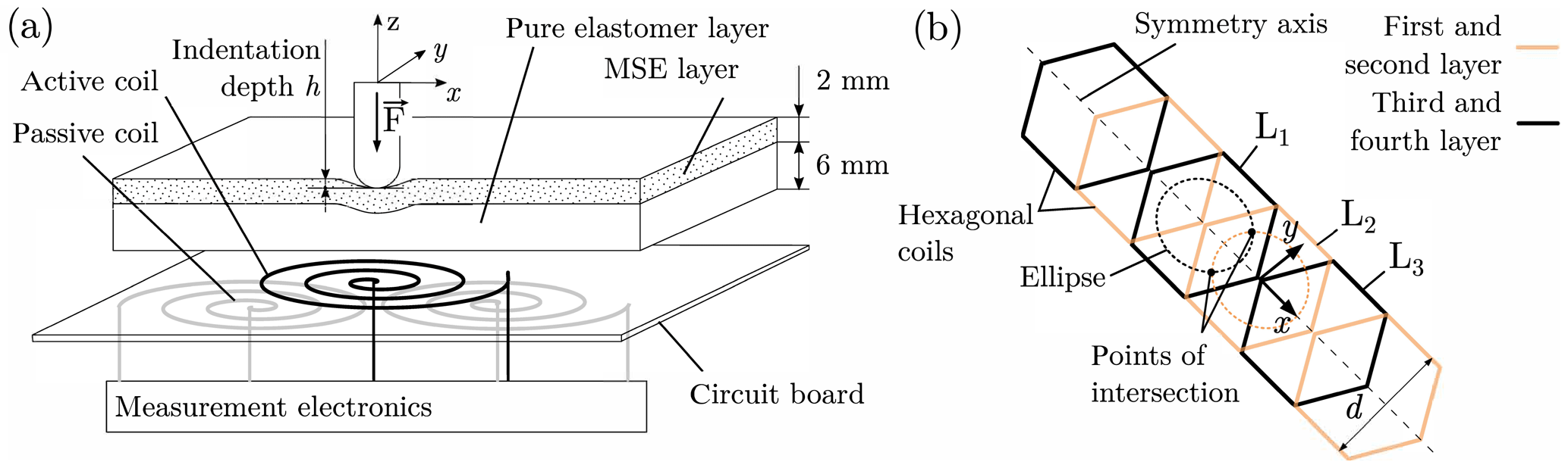
Figure 1(a) Setup of the tactile sensor concept. (b) Linear coil array of the prototype containing six hexagonal planar coils.
We use silicone rubber as the basis material for the sensing layer, since this material does not interact magnetically with the coils, is well investigated and allows large deformations. The operating distance of inductive proximity sensors utilizing planar coils is restricted to the dimensions of the coil diameter. Thus, we chose the sensing layer thicknesses in the same range. As filler material, carbonyl iron powder is inserted, due to its magnetically soft characteristics. Furthermore, the particles are electrically nonconductive; thereby, eddy currents in the sensing layer are avoided.
2.2 Working principle
Since the MSE contains iron particles, its relative magnetic permeability is greater than that of air and the one of the pure elastomer layer. First, we consider an indentation of depth h in the negative z direction, as shown in Fig. 1a. In case the indentation is in a certain interval of the x and y position, the magnetic flux density and, thus, the inductance of a spiral coil is increased. We suppose that the inductance change in every coil depends on three variables, namely the indentation depth h, the x position and the y position of the indenter. As a first approach, a constant value of indentation depth h is used.
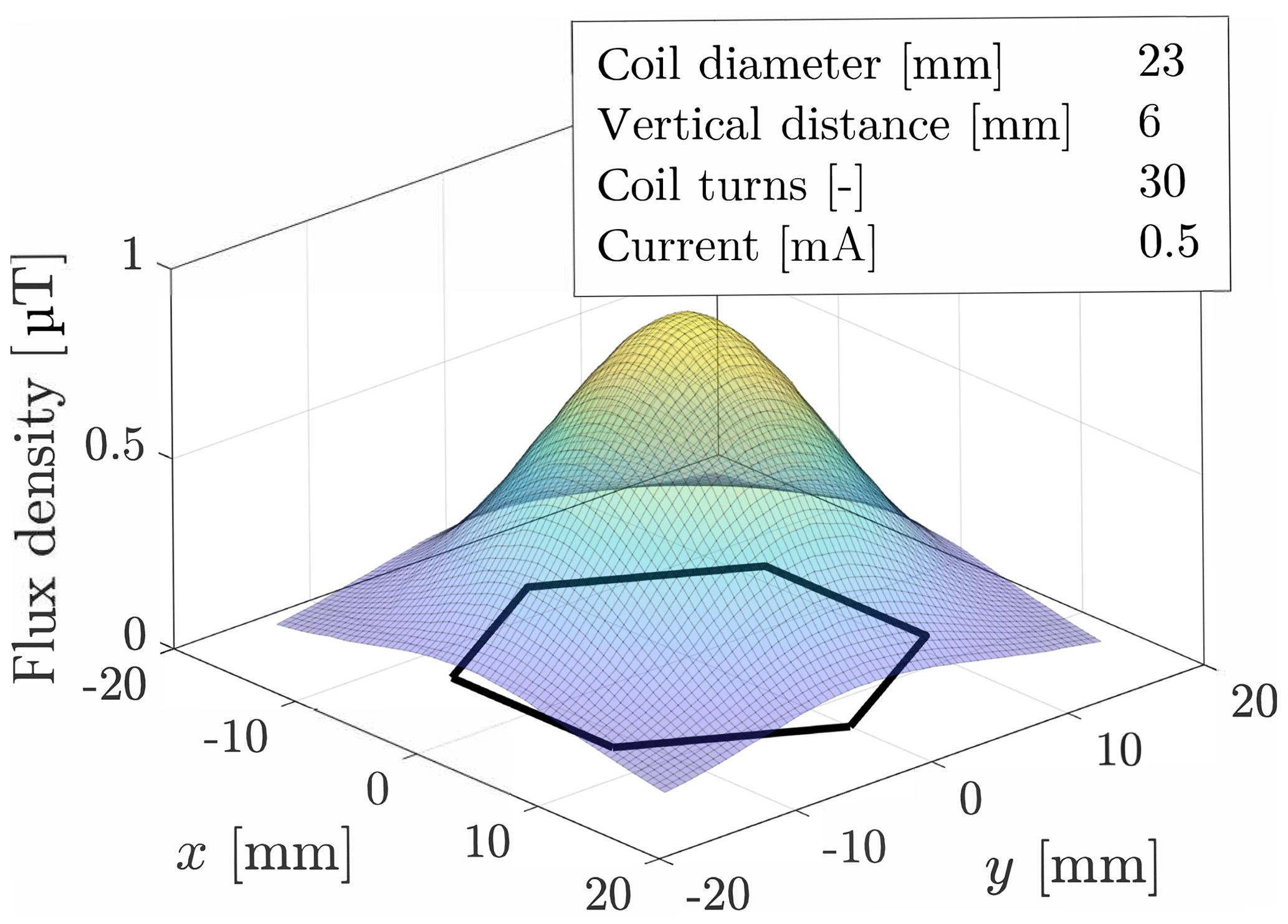
According to Biot–Savart's law, the magnitude of flux density at a given distance, in the z direction, to a single coil can be approximated with a bell-shaped curve (Fig. 2). We assume the inductance change curve of a planar-shifted indentation with constant depth h to be similar to this function. As a result, the peak value of the inductance change occurs in the center of a coil. Considering a horizontal slice through a bell-shaped curve, for example, for a given inductance change value, a circle-like function is obtained. Here, this function is fitted with an ellipse. The mathematical model for this approximation is described in detail in Sect. 4. Measuring two coils for the same indentation results in two ellipses. Since the coils overlap each other, both ellipses intersect. The points of intersection have the same x coordinate. The absolute value of the y coordinates is equal as well. However, due to its symmetry, the system is not able to distinguish the points of intersection. The mathematical model presented in Sect. 4 provides the coordinates of both points of intersection. Thus, the x position of the indentation is obtained.
2.3 Electronics
The main part of the measurement electronics is an inductance-to-digital converter operating in single channel mode (LDC1614 evaluation module; Texas Instruments). This module uses a closed loop control to ensure an adjustment of the frequency in order to maintain resonance. This frequency corresponds to the inductance (Eq. 1) by assuming that the remaining electric components are unchanging. Hence, the inductance of an oscillating circuit can be evaluated by recording the frequency at a very high resolution.
Here, f0 corresponds to a parallel circuit of an ideal capacitance C and an ideal inductance L. Another module incorporates multiple analogue multiplexers (ADG739; complementary metal–oxide–semiconductor (CMOS) analog matrix switch; Analog Devices). Thus, all terminals of the coils can be switched between three states, namely the ground channel, high-resistance channel and measurement channel. Additionally, a microcontroller (XMC 2Go Kit with an XMC1100; Infineon Technologies) is used to define the states of the multiplexer and trigger measurements and pass data to a computer. Each coil of the array is sampled sequentially. During the time a coil is excited (active coil), the remaining coils (passive coils) are connected to the ground potential. The sampling time for all six inductances is 0.2935 s. Due to Lenz's law, the passive coils create magnetic fields, which counteract the magnetic field of the active coil. This interference lowers the inductance of the active coil and may restrict the area of measurable response for each coil. Hence, a small coupling coefficient between the active and passive coil is preferable. From this effect, one requirement is deduced, namely that an indentation occurring at small distances outside of the dimensions of a single coil must still cause a measurable response. Thus, sufficient data are available for obtaining intersecting ellipses in the entire x interval between the two center points of overlapping coils (see Sect. 2.2).
3.1 Experimental setup
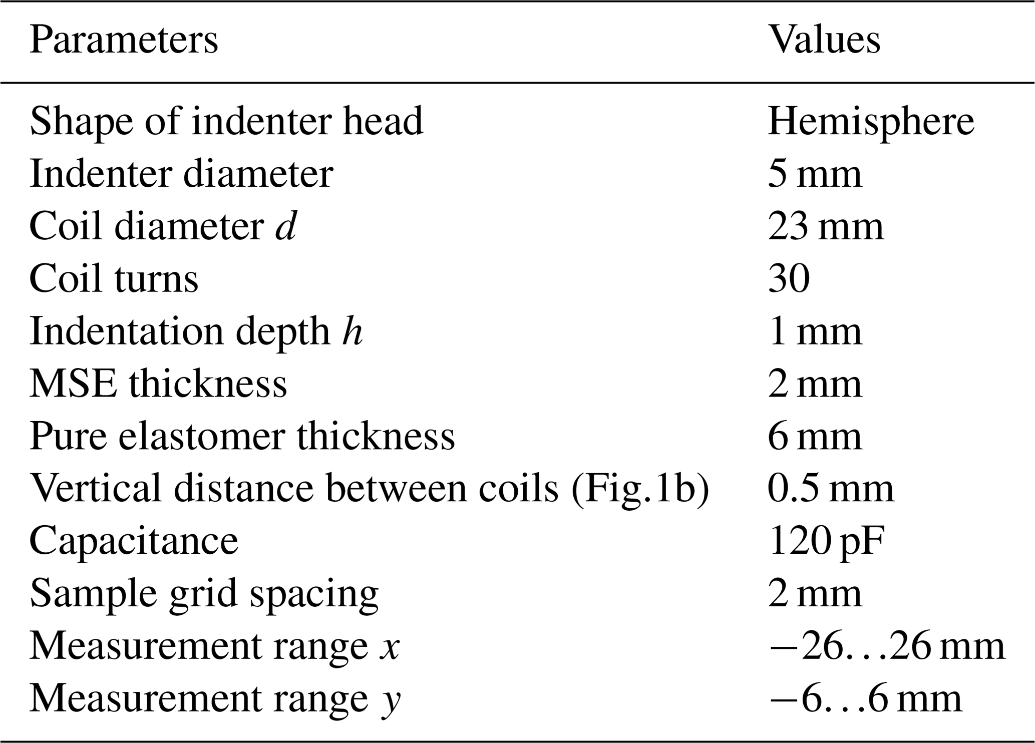
As shown in Fig. 3, the experimental setup consists of the fixed sensor and three linear axes holding the indenter. The indenter deforms the MSE sample in normal direction to the surface with constant maximum indentation. The other two axes alternate the planar position. Referring to the 100 mm movement of an axis, the vertical positioning deviates by 35 µm and the other axis deviates by 25 µm. All parameters of the experiments are listed in Table 1.

3.2 Fabrication of the elastomer layers
The MSE layer is composed of 30 % volume fraction of carbonyl iron powder (average particle size of 6.5…10 µm; grade CEP CC; BASF) and 70 % volume fraction room temperature vulcanizing addition cross-linking silicone rubber (Ecoflex® Shore 00-20; Smooth-On, Inc.). The elastomer base layer consists of the same pure silicone rubber. Both mixtures were degassed in a vacuum chamber before curing. To ensure interconnection of the compound, the MSE layer was vulcanized on the cured pure elastomer base.
3.3 Sensor response sampling
At the beginning of the measurements, the reference z position of the elastomer sample is identified by evaluating the point of contact with the force sensor. The grid and range for the sampling are listed in Table 1. To eliminate dynamic effects, the deformation in the z direction is performed at low velocities. The sampling of the sensor is executed with the following looped sequence:
-
Move to a planar position (elastomer is relaxed)
-
Indent at −1.5 mm s−1 until maximum depth h in z direction
-
Allow residence time of 0.5 s
-
Relax the sample at 1.5 mm s−1 in z direction until contact is released.
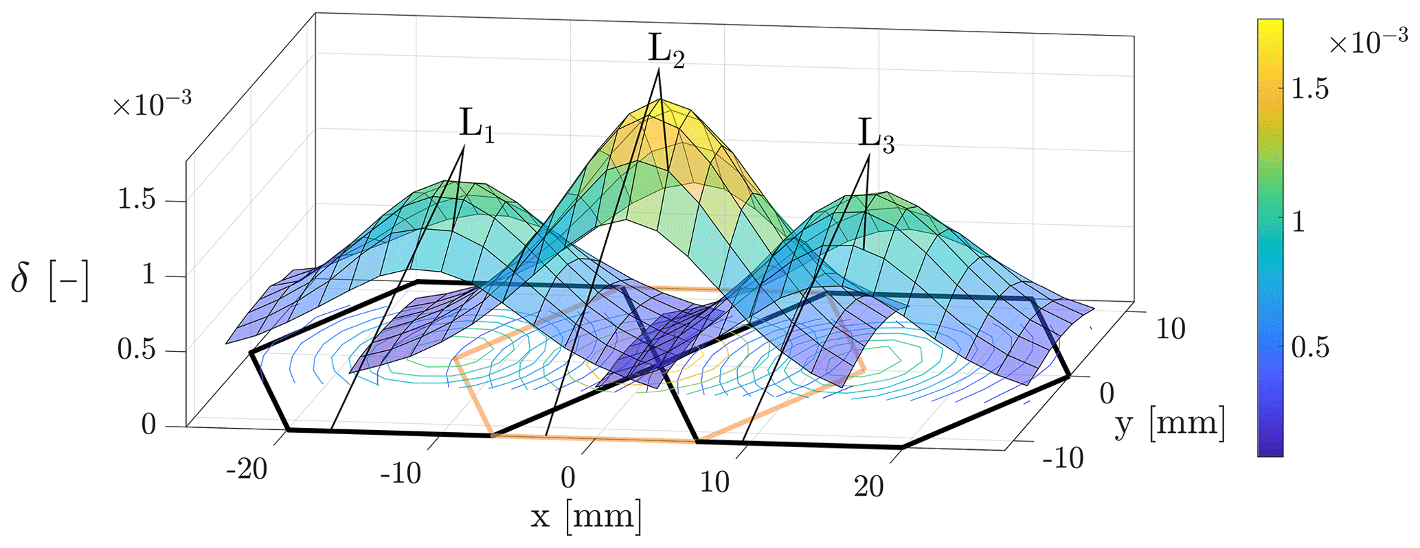
As a first approach, we evaluate and model the inductances of the coils Li, i=1…3 (see Fig. 1b). All other coils are operated as well. However, they are not included in the evaluation process. Since the structure of the sensor is repetitive, the sensor and model are extendable. The dimensionless inductance change value δ is calculated by the following:
Here, Li,peak corresponds to the inductance value of maximum indentation h (step 3 of the sampling sequence above), and Li,0 is the inductance value of the undeformed state. For each coil, all values of δ are stored in a sensor response matrix (SRM). These values meet the requirement in Sect. 2.3 and occur outside the dimensions of each coil in the x direction (see Fig. 4).
The sensor response in the chosen region is modeled with Eqs. (3) and (4). Firstly, we assume symmetric sensor response values with respect to the two symmetry planes of the planar coils that are aligned perpendicularly to the x and y axes. Therefore, Eq. (3), representing an ellipse, is always centered on the y axis and is not tilted. Thus, the parameters x0, i, Ai and Bi represent the center position in the x direction, the semiaxis in the x direction and the semiaxis in the y direction of an ellipse.
In Sect. 5, the parameters x0, i, Ai and Bi are fitted with a polynomial to the SRM of each coil. We chose a polynomial f(δ) of the fourth degree, due to the nonlinear trend and inflection points of the parameters (see Fig. 5b). Thus, the fit is a compromise between model complexity and accuracy. Additionally, an analysis of the root mean square error of the polynomial fits of higher degrees does not lead to significantly more accuracy.
Considering two intersecting ellipses, we obtain a system of two quadratic equations for x and y. In general, those equations result in up to four solutions, including two imaginary and two real solutions for y. Here, we only evaluate the solutions of the equations that lead to real numbers. Thus, the x coordinate can be estimated by solving the system of equations for x. The quadratic polynomial for x delivers two solutions. Referring to the restricted domain , there is only one solution for x.
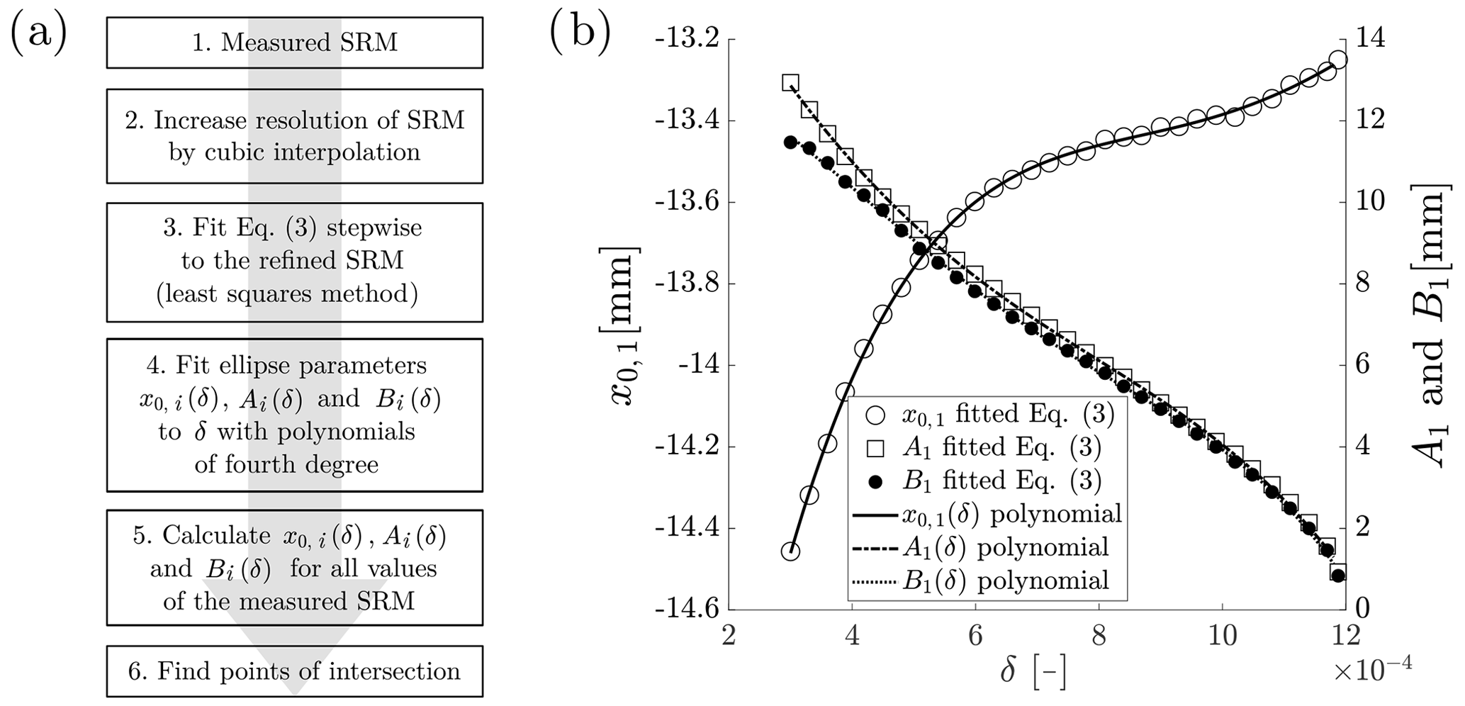
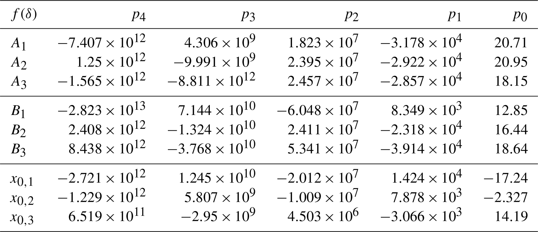
All data postprocessing is done with MATLAB R2018b. The stepwise sequence of the script is shown in Fig. 5a. Firstly, the resolution of the SRM is refined by cubic interpolation to obtain a higher resolution. Next, a stepwise sweep through the data of the refined SRM is done, fitting Eq. (3) to the values of each step (Gal, 2003). The steps are executed with a threshold of and a step size of of δ. This leads to a set of ellipses for each coil, obtaining x0, i, Ai and Bi for each step. Subsequently, we use polynomials of the fourth degree (Eq. 4) to fit these ellipse parameters with a dependency on δ. Here, δ is calculated from the mean value of each step. The values for pk of the functions Ai(δ), Bi(δ) and x0, i(δ) are listed in Appendix A. For the coil L1, the results of the data processing are plotted in Fig. 5b. The markers represent the ellipse parameters of each fit of Eq. (3) to the refined SRM. The lines in different styles depict the fit of the polynomials A1(δ), B1(δ) and x0, 1(δ) (Eq. 4). For each indentation, the evaluation of Ai(δ), Bi(δ) and x0, i(δ) of two overlapping coils leads to two intersecting ellipses. As a last step, the x components of the points of intersection are calculated (see Sect. 4).
In Fig. 6, three cases of intersecting ellipses are shown. The procedure described in the previous paragraph commonly results in the first case. Cases two and three are special cases that need to be considered separately. An indentation close to y=0 leads to a single point where the ellipses touch (case two). An indentation in the area around the coil center (case three) results in . Consequently, the semiaxes are equal, leading to a circle with a small radius (see Figs. 5b and 6). Due to measurement and interpolating errors, both cases possibly lead to curves with no intersection. In order to avoid such cases, a constant value of 0.2 mm is added to all polynomials for the semiaxis Ai(δ). Although the values of the points of intersection are thus changed, potential cases with no intersection are avoided. Secondly, in the area close to the coil center, the points of intersection are found by evaluating the two adjacent inductances.
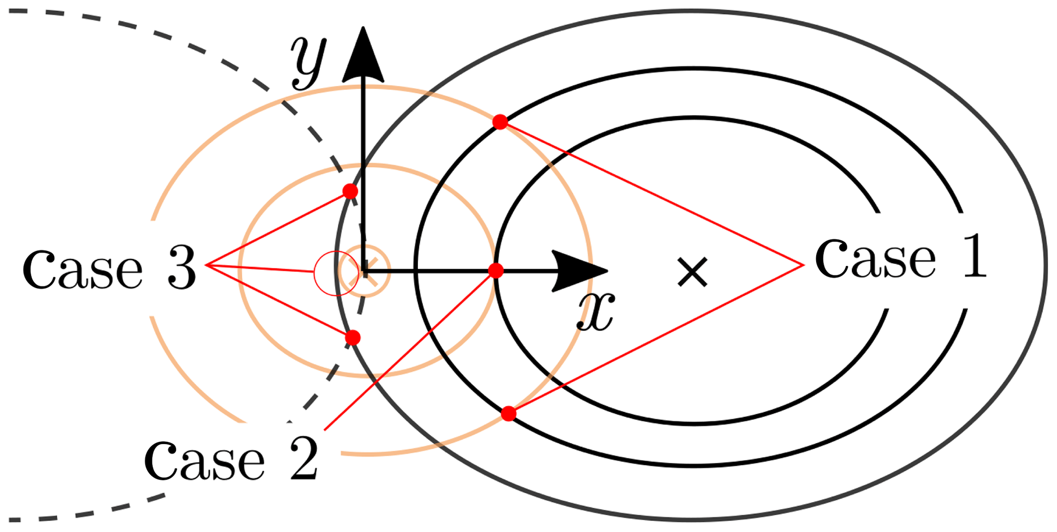
The polynomial fit of each ellipse parameter has an intercept of zero for a value of . Since the sample grid spacing is finite, this δ value might be reached for indentations close to the center of a coil. However, the distinction of the three cases described in Sect. 5 means avoiding such cases (see Fig. 6). Furthermore, the semiaxes appear to tend to infinity for small values of δ. Due to measurement noise, the smallest measurable value of δ is greater than zero and leads to a finite length of the semiaxis. For the measurement concept, those values are neglectable since in that range the inductance values δ of adjacent coils are significantly higher.

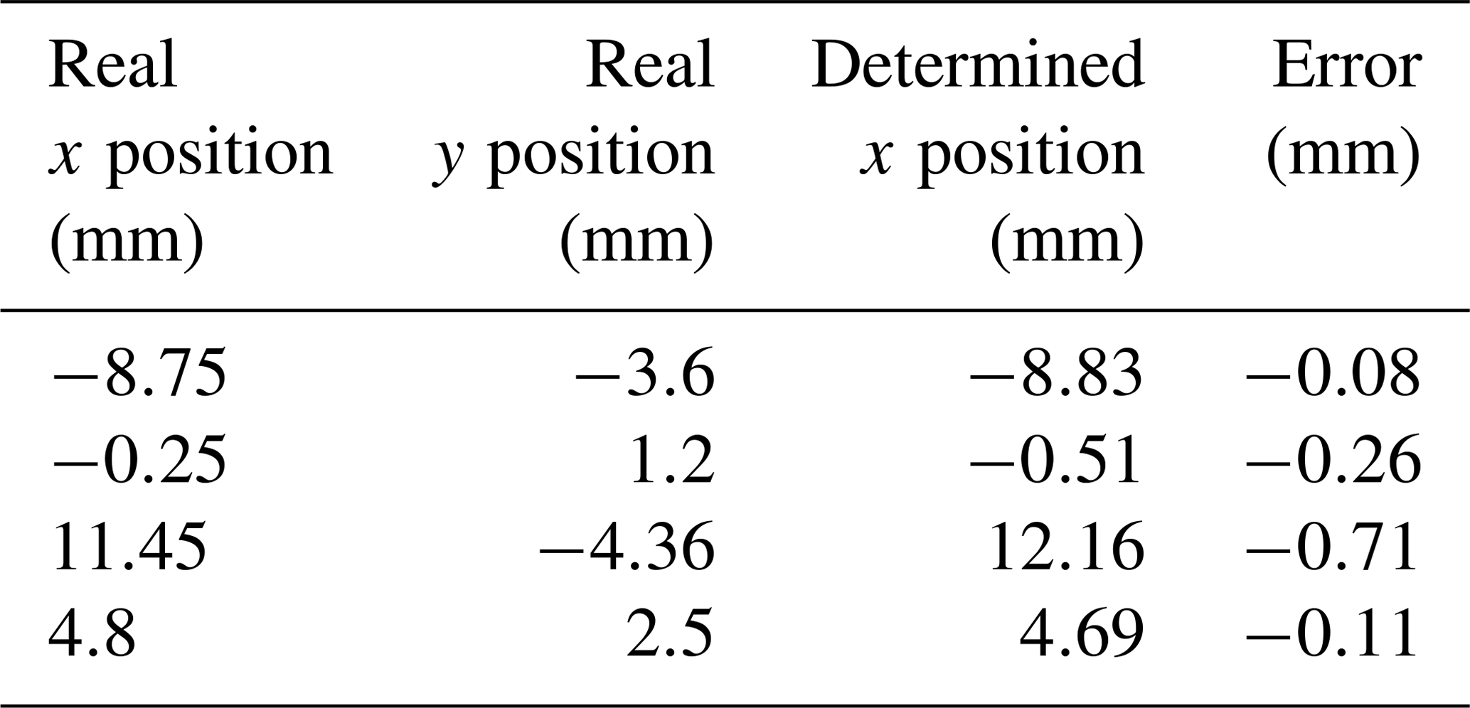
As a first approach, we use the initial sample grid measurements to calculate the deviation of the determined x coordinate (Sect. 5) from the real position of the indenter. The absolute error of the position is less than 0.8 mm (Fig. 7). Thus, errors caused by the polynomial fit and fitting ellipses to the refined SRM are determined. This deviation is also increased by the constant value we added to all semiaxes, namely Ai(δ). Furthermore, four additional measurements at random positions are done, nonrecurringly, to check the model at points that are not covered by the sampling of the sensor (see Table 2). For these measurements, the maximum error is at −0.71 mm. Hence, we conclude that this model can be applied to any planar position of the indenter in the measurement range and with the equal indentation h. For the validation of the model, more measurements are necessary at positions that are not covered by the sampling of the sensor and that are assured with repeatability tests.
Table 2Four measurements at random positions to determine the x position.
For the proposed model and the determination of the position, it is a crucial requirement that the indenter shape and indentation depth h are not variable. The nature of the method is to model the sensor response based on a wide data set. Considering an indentation of variable depth and the indenter shape, the sampling and modeling of the sensor is rather complex. In this case, other model approaches are preferable. However, investigating the rate of the inductances of two overlapping coils is a promising approach, for instance.
Although the trend of the semiaxes Ai(δ) and Bi(δ) are similar, the trend of x0, i differs from L1 to L3. Depending on which coil is active, the relative asymmetrical arrangement of the passive coils changes. Thus, the spatial distribution of the flux density is distorted in a different manner by the opposing magnetic fields (passive coils). This leads to different trends of x0, i. To avoid this effect, the sensor can be optimized by means of geometric variations of the coil array in order to minimize the coupling coefficient.
The inductance measurements are based on high-frequency magnetic fields (≈2 MHz) at very low amplitudes. Hence, an external quasi-static magnetic field will not influence the inductance measurements, assuming that the flux density in the MSEs does not reach saturation and that the relative magnetic permeability is constant. This external magnetic field can be used to obtain a tunable stiffness. Thus, the sensor is possibly able to perform tactile measurements and control the stiffness simultaneously.
The setup of measurement electronics allows an interconnection of multiple coils by using the analogue multiplexer. Hence, the magnetic flux density distribution can be varied by using parallel or series connections of overlapping coils. This results in a larger response area compared to a single coil. Additionally, this method may be used to improve the accuracy of the sensor.
The proposed tactile sensor concept offers versatile fields of application, ranging from gripping to tactile control systems. As a first realized approach, we present a linear coil array that is adequate for the position determination, in one direction, of an indentation of constant depth. The analysis shows that the individual measurement of every coil provides sufficient data for sampling and modeling. The model formed by ellipse equations, with three parameters each and a polynomial fit, results in an absolute position determination error of less than 0.8 mm. Furthermore, the coupling of the coil array results in a distorted flux density distribution. This distortion is modeled mainly by the ellipse parameter x0, i.
Subsequent investigation will focus on expanding the control concepts and evaluation methods in order to determine the planar position. Such experiments will be executed with variable depths of indentation and will be extended to analyze the repeatability of the performance. Additionally, we will optimize the coil array regarding the coupling coefficients. Furthermore, we will add a quasi-static external magnetic field to the setup to investigate a simultaneous control of the stiffness.
The sampling data and the four measurements at random positions are accessible at https://doi.org/10.17605/OSF.IO/BV6P4 (Gast, 2020).
SG was responsible for the sensor concept, elastomer sample fabrication, measurements, mathematical modeling, data processing and writing the paper. KZ supervised the work, with the support of the Technische Universität Ilmenau Technical Mechanics Group, and approved the final paper.
The authors declare that they have no conflict of interest.
This article is part of the special issue “Sensors and Measurement Science International SMSI 2020”. It is a result of the Sensor and Measurement Science International, Nuremberg, Germany, 22–25 June 2020.
The authors would like to thank the Deutsche Forschungsgemeinschaft (DFG), within the PAK 907 project, and Moritz Scharff and Marek Ziolkowski (both at Technische Universität Ilmenau) for their critical remarks and support.
This research has been supported by the Deutsche Forschungsgemeinschaft (DFG; grant no. ZI 540/17-3).
This paper was edited by Eric Starke and reviewed by two anonymous referees.
Boie, R. A.: Capacitive impedance readout tactile image sensor, Proceedings IEEE International Conference on Robotics and Automation, 13–15 March 1984, Atlanta, GA, USA, 370–378, 1984. a
Custy, E. J.: Apparatus and method for incorporating tactile control and tactile feedback into a human-machine interface, US patent 7,245,292 B1, 2007. a
De Maria, G., Natale, C., and Pirozzi, S.: Force/tactile sensor for robotic applications, Sensor. Actuat. A-Phys., 175, 60–72, 2012. a
Drimus, A., Kootstra, G., Bilberg, A., and Kragic, D.: Design of a flexible tactile sensor for classification of rigid and deformable objects, Robot. Auton. Syst., 62, 3–15, 2012. a
Gal, O.: Ellipse fit function from point sets, MATLAB Central File Exchange, available at: https://de.mathworks.com/matlabcentral/fileexchange/3215-fit_ellipse (last access: 23 September 2020), 2003. a
Gast, S.: Tactile Sensor Data, Open Science Framework, https://doi.org/10.17605/OSF.IO/BV6P4, 2020. a
Günther, L., Becker, F., Becker, T. I., Stepanov, G. V., and Zimmermann, K.: Development of an acceleration sensor incorporating a magneto-sensitive elastomer, 59th IWK, Ilmenau Scientific Colloquium, 11–15 September 2017, Technische Universität Ilmenau, Germany, 2017. a
Kawasetsu, T., Horii, T., Ishihara, H., and Asada, M.: Size dependency in sensor response of a flexible tactile sensor based on inductance measurement, 29 October–1 November 2017, Glasgow, UK, IEEE Sensors, 1–3, 2017. a
Kawasetsu, T., Horii, T., Ishihara, H., and Asada, M.: Flexible Tri-Axis Tactile Sensor Using Spiral Inductor and Magnetorheological Elastomer, IEEE Sens. J., 18, 5834–5841, 2018. a
Li, R., Zhou, M., Wang, M., and Yang, P.: Study on a new self-sensing magnetorheological elastomer bearing, AIP Advances, 28, 1–8, 2018. a
Li, Y., Li, J., Tian, T., and Li, W.: A highly adjustable magnetorheological elastomer base isolator for applications of real-time adaptive control, Smart Mater. Struct., 22, 1–24, 2013. a
Massari, L., Schena, E., Massaroni, C., Saccomandi, P., Menciassi, A., Sinibaldi, E., and Oddo, C. M.: A Machine-Learning-Based Approach to SolveBoth Contact Location and Force in Soft Material Tactile Sensors, Soft Robotics, 7, 1–12, 2019. a
Qi, S., Guo, H., Chen, J., Fu, J., Hu, C., Yu, M., and Wang, Z. L.: Magnetorheological elastomers enabled high sensitive self-powered tribo-sensor for magnetic field detecting, Nanoscale, 10, 4745–4752, 2018. a
Yoo, B., Na, S., Flatau, A. B., and Pines, D. J.: Evaluation of Magnetorheological Elastomers With Oriented Fe–Ga Alloy Flakes for Force Sensing Applications, IEEE T. Magn., 52, 1–4, 2016. a
- Abstract
- Introduction
- Sensor prototype
- Experiments
- Mathematical model
- Determination of the x position
- Discussion
- Conclusion and future work
- Appendix A: Interpolation parameters pk
- Data availability
- Author contributions
- Competing interests
- Special issue statement
- Acknowledgements
- Financial support
- Review statement
- References