Measurement uncertainty assessment for virtual assembly

Virtual assembly (VA) is a method for datum definition and quality prediction of assemblies considering local form deviations of relevant geometries. Point clouds of measured objects are registered in order to recreate the objects' hypothetical physical assembly state. By VA, the geometrical verification becomes more accurate and, thus, increasingly function oriented. The VA algorithm is a nonlinear, constrained derivate of the Gaussian best fit algorithm, where outlier points strongly influence the registration result. In order to assess the robustness of the developed algorithm, the propagation of measurement uncertainties through the nonlinear transformation due to VA is studied. The work compares selected propagation methods distinguished from their levels of abstraction. The results reveal larger propagated uncertainties by VA compared to the unconstrained Gaussian best fit.

1 Current trends in dimensional metrology and state-of-the-art datum definition and uncertainty assessment

As quality demands on products increase, tolerance specifications for parts become more and more complex. With these challenging geometrical specifications, verification algorithms are required that represent the geometrical system more precisely. According to Nielsen (2003), in the last few decades, dimensional tolerances shrank due to improved manufacturing systems. However, the form deviations could not be reduced by the same extent. Therefore, their consideration should be intensified. A main deficit in the current International Organization for Standardization (ISO) standard for datum definition, ISO 5459 (Deutsches Institut für Normung e.V., 2011), is the lack of consideration of local form deviations for datum features. A datum feature is defined as a “real (non-ideal) integral feature used for establishing a single datum” (Deutsches Institut für Normung e.V., 2017, p. 2). Datum systems composed of three datum features mathematically define a coordinate system. This allows the definition of tolerance zones for extrinsic tolerances (Weißgerber and Keller, 2014). About 80 % of all measurement tasks require datum systems, so a further function-oriented datum system definition has a strong impact on geometrical verification. Hence, an assessment of the uncertainty for datum systems is of broad interest. Figure 1 shows a datum definition, where three perpendicular associated planes are considered in a nested approach. The primary datum constrains 3 degrees of freedom (DOF), the secondary datum 2 DOF and the tertiary datum 1 DOF (Gröger, 2015).

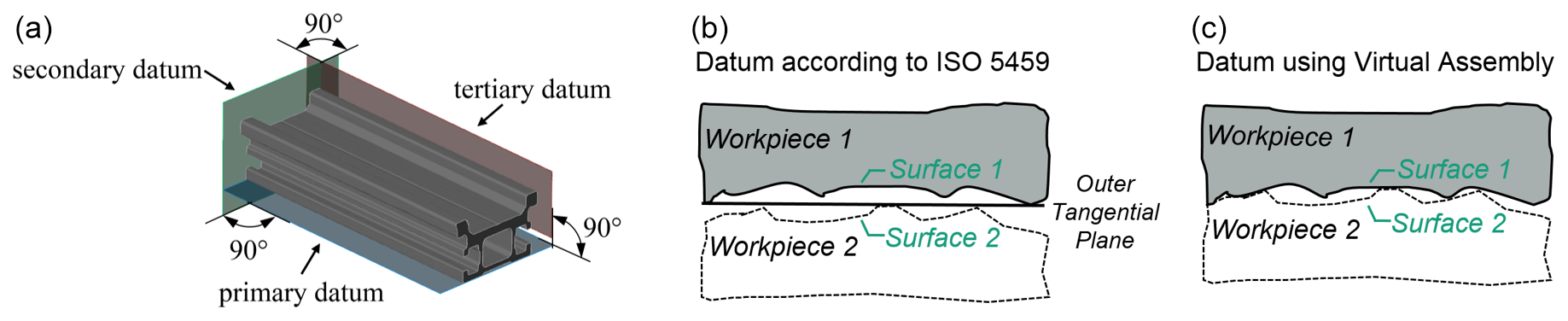
Figure 1 Datum definition by nested registration, using associated planes (a), registration approach according to the default case in the current standard, (b) and registration approach according to virtual assembly (c).

1.1 Concept of the virtual assembly

In this paper, measurement data of physical objects are gathered from measurements using industrial computed tomography (CT). Registration is the action of aligning a data set relatively to another according to a datum definition in a common coordinate system. Virtual assembly (VA) comprises the consideration of local form deviations in the datum system computation. As shown in Fig. 1a, through VA, the physical workpiece contact is simulated by computing the contact points. The registration for VA is mathematically stated as an optimization problem, as introduced in Weißgerber and Keller (2014). In the following, matrices are marked as boldface capital, vectors in boldface italic, and scalar values in roman formatting. The signed distances d_sig,i of i∈1…N, $i\in {\mathbb{N}}^{+}$, corresponding pairs of points $\left\{p_{\mathrm{1},i},p_{\mathrm{2},i}\right\}$, with $p_{\mathrm{1},i}\in {\mathit{P}}_{\mathrm{1}}$ and $p_{\mathrm{2},i}\in {\mathit{P}}_{\mathrm{2}}$ determine the clearance between the surfaces to register. P₁ and P₂ are point sets of surfaces 1 and 2, respectively, as presented in Fig. 1b and c. The objective function f of the optimization problem is as follows:

$$\begin{array}{}\text{(1)}& f\left(t_x,t_y,t_z,\mathit{\varphi },\mathit{\theta },\mathit{\psi }\right)=\sum _{i=\mathrm{1}}^N{d}_{\text{sig},i}^{\mathrm{2}}=\text{min!},\end{array}$$

where the sum of the squared signed distances d_sig is minimized. The optimization variables t_x, t_y, and t_z determine the translation, and ϕ, θ, and ψ are the Euler angles of the rigid transformation of the point set to register P₂ to the fixed point set P₁. The avoidance of a physical intersection of parts is formulated as the omission of surface intersection, where ${\mathit{P}}_{\mathrm{1}}\cap {\mathit{P}}_{\mathrm{2}}=\mathrm{\varnothing }$.

This optimization constraint can be either formulated as a hard constraint, as implemented in this work, allowing $d_{\text{sig},i}\ge \mathrm{0}$ only, or by a soft constraint by introducing a penalty term in order to permit small intersections. However, the constrained optimization is formulated as an unconstrained, differentiable optimization problem by using the Lagrange multiplier method (Griva et al., 2009). Thus, a Lagrange function ℒ, according to the following:

$$\begin{array}{}\text{(2)}& \begin{array}{rl}\mathcal{L}\left(\mathbf{M},\mathit{\lambda }\right)& =f\left(\mathbf{M}\right)+\mathit{\lambda }\cdot g\left(\mathbf{M}\right)=\sum _{i=\mathrm{1}}^N{d}_{\text{sig},i}^{\mathrm{2}}\\ & +\mathit{\lambda }\cdot \sum _{j=\mathrm{1}}^{N_{\text{neg}}}{d}_{\text{sig},\text{neg},j},\end{array}\end{array}$$

with λ as the Lagrange multiplier and g(M) as sum of squared negative signed distances $d_{\text{sig},\text{neg},j}$ is introduced, where $j\in \left[\mathrm{1};N_{\text{neg}}\right]$, $j\in {\mathbb{N}}^{+}$, and $N_{\text{neg}}=\left|D_{\text{sig},\text{neg}}\right|$ is the cardinality of the set of negative signed distances $D_{\text{sig},\text{neg}}=\left\{d_{\text{sig}}\mid d_{\text{sig}}<\mathrm{0}\right\}$ for a particular transformation $\mathbf{M}\left(t_x,t_y,t_z,\mathit{\varphi },\mathit{\theta },\mathit{\psi }\right)$. The first-order optimality condition can be stated as ∇L=0. The transformation of each point p_2,i of the point set P₂ from its initial scene coordinate system into the transformed world coordinate system, defined by the datum system and, in the following, denoted by superscript Tr, is defined as follows:

$$\begin{array}{}\text{(3)}& {\mathit{P}}_{\mathrm{2}}^{\mathbf{\text{Tr}}}=\mathbf{M}\cdot {\mathit{P}}_{\mathrm{2}}=\left(\mathbf{R}+\mathbf{T}\right)\cdot {\mathit{P}}_{\mathrm{2}},\end{array}$$

where ${\mathit{P}}_{\mathrm{2}}^{\mathbf{\text{Tr}}}$ is the transformed point set, R is the rotation matrix gathered by matrix multiplication of the individual rotation matrices for ϕ, θ, and Ψ in the named order, T is the translation matrix with its components t_x, t_y, and t_z, and M is the composed transformation matrix. The signed distances d_sig,i are determined according to the following:

$$\begin{array}{}\text{(4)}& d_{\text{sig},i}=\text{sign}\left({\mathit{n}}_i^T\cdot {\mathit{P}}_{\mathbf{2}\mathbf{,}\mathit{i}}^{\text{Tr}}{\mathit{P}}_{\mathbf{1}\mathbf{,}\mathit{i}}\right)\cdot {∥P_{\mathrm{2},i}^{\text{Tr}}-P_{\mathrm{1},i}∥}_{\mathrm{2}},\end{array}$$

where n_i is the normal vector in P_1,i. The optimization problem is nonlinear due to trigonometric functions arising at transformation, as shown in the explicit depiction in matrix notation in Eq. (5) for a point $p_{\mathrm{2},i}\left(p_{\mathrm{2},i,x},p_{\mathrm{2},i,y},p_{\mathrm{2},i,z}\right)$, as per the following:

$$\begin{array}{}\text{(5)}& \begin{array}{rl}\left[\begin{array}{c}{p}_{\mathrm{2},i,x}^{\text{Tr}}\\ p_{\mathrm{2},i,y}^{\text{Tr}}\\ p_{\mathrm{2},i,z}^{\text{Tr}}\\ \mathrm{1}\end{array}\right]& =\left[\begin{array}{cccc}\cos \mathit{\theta }\cdot \cos \mathit{\psi }& -\cos \mathit{\theta }\cdot \sin \mathit{\psi }& \sin \mathit{\theta }& t_x\\ \sin \mathit{\varphi }\cdot \sin \mathit{\theta }\cdot \cos \mathit{\psi }+\cos \mathit{\varphi }\cdot \sin \mathit{\psi }& -\sin \mathit{\varphi }\cdot \sin \mathit{\theta }\cdot \sin \mathit{\psi }+\cos \mathit{\varphi }\cdot \cos \mathit{\psi }& -\sin \mathit{\varphi }\cdot \cos \mathit{\theta }& t_y\\ -\cos \mathit{\varphi }\cdot \sin \mathit{\theta }\cdot \cos \mathit{\psi }+\sin \mathit{\varphi }\cdot \sin \mathit{\psi }& \cos \mathit{\varphi }\cdot \sin \mathit{\theta }\cdot \sin \mathit{\psi }+\sin \mathit{\varphi }\cdot \cos \mathit{\psi }& \cos \mathit{\varphi }\cdot \cos \mathit{\theta }& t_z\\ \mathrm{0}& \mathrm{0}& \mathrm{0}& \mathrm{1}\end{array}\right]\\ & \cdot \left[\begin{array}{c}{p}_{\mathrm{2},i,x}\\ p_{\mathrm{2},i,y}\\ p_{\mathrm{2},i,z}\\ \mathrm{1}\end{array}\right].\end{array}\end{array}$$

1.2 Introduction to measurement uncertainty assessment

A complete statement of a measurement result includes the measurement uncertainty. The measurement uncertainty is a nonnegative quantity expressing doubt about the measured value, defined as a “parameter, associated with the result of a measurement, that characterizes the dispersion of the values that could reasonably be attributed to the measurand” (ISO/IEC, 2008b). In ISO/IEC (2008a), the main stages of uncertainty assessment are described as formulation, propagation, and summarizing. During formulation, generally the measurand Y is defined, input quantities X are determined, and the measurement model is established as follows:

$$\begin{array}{}\text{(6)}& \mathit{Y}=f\left(\mathit{X}\right).\end{array}$$

A main step is the uncertainty estimation for the input quantities. The Guide to the expression of uncertainty in measurement (GUM) (ISO/IEC, 2008b) reveals two methods for uncertainty estimation. With a type A evaluation, statistical quantities from independent, uncorrelated observations are assessed. With a type B evaluation, the uncertainty is estimated based on a priori information, such as specifications, previous measurements, calibration data, or user experience. Since no a priori knowledge is available in this work, the type A evaluation is conducted as described in Sect. 3.1. Uncertainties are separated in systematic and stochastic contributors. Since no calibrated values are available, the systematic error (bias) from a calibrated true value is omitted in this work. During the propagation step, uncertainties assigned to Y are propagated through the measurement model. An overview on propagation methods is given in Sect. 3.2. At the summarizing step, the propagated uncertainty is consolidated into a coverage interval, extended by coverage factor k (ISO/IEC, 2008a).

2 Aim and scope of this paper

The aim of this work is to analyze the uncertainty propagation for the VA algorithm. Since only few contact points may influence the hard constraint of the optimization problem, a lower robustness compared to existing methods is initially assumed. At the moment, uncertainty propagation is commonly not considered for fitting algorithms such as the VA. However, information gathered from the uncertainty propagation could, on the one hand, be used to claim the robustness of a registration result and, hence, the derived measurements. On the other hand, this allows a reduction in the uncertainty contribution of registration algorithms, for example, by avoiding less certain registration results.

As a use case, a linear guide assembly, consisting of a slider mounted to a rail, is assessed, which is shown in Fig. 3. Measurement data were captured using the CT system Werth TomoScope HV 500, with an acceleration voltage of 180 kV, a tube current of 240 mA, an integration time of 500 ms, 1000 projection images, and a resulting voxel size of 0.2 mm.

3 Description of methods for uncertainty assessment and propagation

The propagation model corresponds to the model function ${\mathit{P}}_{\mathrm{2}}^{\mathbf{\text{Tr}}}=\mathbf{M}\cdot {\mathit{P}}_{\mathrm{2}}$ outlined in Eq. (3). Each quantity has an associated uncertainty. The initial uncertainties before propagation comprise the transformation uncertainty u_T, associated to transformation M, and the point uncertainty U_Pt, associated to the point set P₂. The propagated uncertainty U^Tr is associated to the transformed measurement point set ${\mathit{P}}_{\mathrm{2}}^{\mathbf{\text{Tr}}}$. In the following, multiple modalities for the declaration of the propagated uncertainty are introduced. The matrix ${\mathbf{U}}^{\mathbf{\text{Tr}}}=\left[{\mathit{u}}_{\mathbf{x}}^{\mathbf{\text{Tr}}},{\mathit{u}}_{\mathbf{y}}^{\mathbf{\text{Tr}}},{\mathit{u}}_{\mathbf{z}}^{\mathbf{\text{Tr}}}\right]$ comprises the uncertainty components of the x, y, and z coordinates. The composition of the uncertainty components ${\mathit{u}}_{\mathbf{x}}^{\mathbf{\text{Tr}}}$, ${\mathit{u}}_{\mathbf{y}}^{\mathbf{\text{Tr}}}$ and ${\mathit{u}}_{\mathbf{z}}^{\mathbf{\text{Tr}}}$ to the combined standard uncertainty ${\mathit{u}}_{\mathbf{c}}^{\mathbf{\text{Tr}}}$ is defined as follows:

$$\begin{array}{}\text{(7)}& {\mathit{u}}_{\mathbf{c}}^{\mathbf{\text{Tr}}}=\sqrt{{\left({\mathit{u}}_{\mathbf{x}}^{\mathbf{\text{Tr}}}\right)}^{\mathrm{2}}+{\left({\mathit{u}}_{\mathbf{y}}^{\mathbf{\text{Tr}}}\right)}^{\mathrm{2}}+{\left({\mathit{u}}_{\mathbf{z}}^{\mathbf{\text{Tr}}}\right)}^{\mathrm{2}}},\end{array}$$

which allows the representation of multivariate measurands in a scalar value. For the mathematical formulation of the propagation, the uncertainties are stated in form of their corresponding covariance matrices. All uncertainties arise from normal distributions due to a Gaussian distribution of random variables in the measurement process. In Fig. 2, the graphical decomposition of the propagation model is shown. In the following Sect. 3.1, the assessment of the initial uncertainties, U_Pt and u_T, is described. In Sect. 3.2, the propagation to determine U^Tr and ${\mathit{u}}_{\mathbf{c}}^{\mathbf{\text{Tr}}}$ is described.

Figure 2 Graphical decomposition of the propagation model.

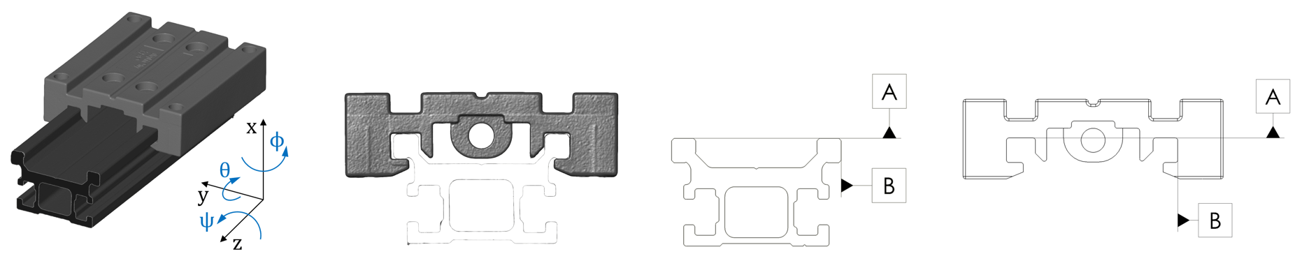
Figure 3 Shown, from left to right, is the 3D representation of the VA, the front view of the assembly, and a technical drawing of the datum system (primary datum A, secondary datum B, and tertiary datum constrained to zero t_z=0 and defined for both the rail and the slider.

3.1 Assessment of the initial uncertainties

The measurement point uncertainty U_Pt associated to P₂ is assessed experimentally by 20 repeated CT scans at constant measurement settings. It is determined according to the single point uncertainty approach proposed by Fleßner et al. (2016). For measurement point i∈1…N, $i\in {\mathbb{N}}^{+}$, the uncertainty matrix is defined according to the following:

$$\begin{array}{}\text{(8)}& {\mathbf{U}}_{\mathbf{\text{Pt}}}=\left[\begin{array}{ccccc}{\mathrm{u}}_{\text{Pt},\mathrm{1},x}& \mathrm{\cdots }& {\mathrm{u}}_{\text{Pt},i,x}& \mathrm{\cdots }& {\mathrm{u}}_{\text{Pt},N,x}\\ {\mathrm{u}}_{\text{Pt},\mathrm{1},y}& \mathrm{\cdots }& {\mathrm{u}}_{\text{Pt},i,y}& \mathrm{\cdots }& {\mathrm{u}}_{\text{Pt},N,y}\\ {\mathrm{u}}_{\text{Pt},\mathrm{1},z}& \mathrm{\cdots }& {\mathrm{u}}_{\text{Pt},i,z}& \mathrm{\cdots }& {\mathrm{u}}_{\text{Pt},N,z}\end{array}\right].\end{array}$$

The column components ${\mathrm{u}}_{\text{Pt},i,x}={\mathrm{u}}_{\text{Pt},i,y}={\mathrm{u}}_{\text{Pt},i,z}={\mathrm{u}}_{\text{Pt},i}$ are equal, since the used uncertainty assessment approach does not allow the consideration of a probing direction.

The uncertainty u_Pt,i equals the standard deviation s_Pt,i of the normally distributed distances d_v,i that are gathered from the 20 scan repetitions v∈1…V, with ${\stackrel{\mathrm{‾}}{d}}_i$ as the average distance of all repetitions for each particular point index i, according to the following:

$$\begin{array}{}\text{(9)}& u_{\text{Pt},i}={\mathrm{s}}_{\text{Pt},i}=\sqrt{{\displaystyle \frac{\mathrm{1}}{V-\mathrm{1}}}\sum _{v=\mathrm{1}}^V{\left(d_{v,i}-{\stackrel{\mathrm{‾}}{d}}_i\right)}^{\mathrm{2}}}.\end{array}$$

In order to calculate the Euclidean norm, as follows:

$$\begin{array}{}\text{(10)}& d_{v,i}={∥p_{v,m}-{\stackrel{\mathrm{‾}}{p}}_i∥}_{\mathrm{2}},\end{array}$$

which is referring to the average point ${\stackrel{\mathrm{‾}}{p}}_i$, corresponding sets of points $\left\{{\stackrel{\mathrm{‾}}{p}}_i,p_{v,m}\right\}$ are gathered by a k-nearest-neighbors spatial search that identifies the indices m in p_v corresponding to each i in ${\stackrel{\mathrm{‾}}{P}}_i$. ${\stackrel{\mathrm{‾}}{P}}_i$ denotes the point set of average points ${\stackrel{\mathrm{‾}}{p}}_i\in {\stackrel{\mathrm{‾}}{P}}_i$ that are the mean coordinates of all repetitions v determined for each i. The uncertainty of transformation is as follows:

$$\begin{array}{}\text{(11)}& {\mathit{u}}_{\mathbf{T}}=\left[{\mathrm{u}}_{\mathrm{T},x},{\mathrm{u}}_{\mathrm{T},y},{\mathrm{u}}_{\mathrm{T},z},{\mathrm{u}}_{\mathit{\varphi }},{\mathrm{u}}_{\mathit{\theta }},{\mathrm{u}}_{\mathit{\psi }}\right],\end{array}$$

and it includes the uncertainties of the optimization variables that are stated in Eq. (1). If u_T is small, a high repeatability of registration results can be assumed. The uncertainty u_T is assessed by a Monte Carlo propagation, according to ISO/IEC (2008a), as the standard deviations of the optimization variables from K=10 000 repetitions, where the point set P₂ is slightly transformed with the delta transformation as follows:

$$\begin{array}{}\text{(12)}& \mathit{\delta }\mathbf{T}=\left[\mathit{\delta }{t}_x,\mathit{\delta }{t}_y,\mathit{\delta }{t}_z,\mathit{\delta }\mathit{\varphi },\mathit{\delta }\mathit{\theta },\mathit{\delta }\mathit{\psi }\right].\end{array}$$

The small transformations in δT are random realizations from a population 𝒩(0,σ_T) for the translations t_x, t_y, t_z and 𝒩(0,σ_R) for rotations ϕ, θ, and ψ. In this work, based on scientific judgment (type B evaluation according to ISO/IEC, 2008a), the values σ_T=0.1 mm and σ_R=0.001 rad are applied. The mean transformation of all K observations is considered as the true transformation, as follows:

$$\begin{array}{}\text{(13)}& \stackrel{\mathrm{‾}}{\mathit{T}}=\left[{\stackrel{\mathrm{‾}}{t}}_x,{\stackrel{\mathrm{‾}}{t}}_y,{\stackrel{\mathrm{‾}}{t}}_z,\stackrel{\mathrm{‾}}{\mathit{\varphi }},\stackrel{\mathrm{‾}}{\mathit{\theta }},\stackrel{\mathrm{‾}}{\mathit{\psi }}\right].\end{array}$$

3.2 Uncertainty propagation method

For the mathematical formulation of the propagation, the variance–covariance matrix Σ (hereafter just covariance matrix) is introduced. Generally speaking, this quadratic matrix comprises the uncertainties u_l,m in form of their variances ${\mathrm{s}}_{l,m}^{\mathrm{2}}={\mathrm{u}}_{l,m}^{\mathrm{2}}$, where the diagonal entries for l=m represent the variances, and correlations are expressed by the covariances for l≠m. The covariances are zero because the input variables are assumed to be uncorrelated, according to Galovska et al. (2012). Eigenvectors and eigenvalues of Σ describe a rotational uncertainty ellipsoid, as shown in Fig. 4. For the generic measurement model Y=f(X), the covariance matrix Σ_x is propagated into Σ_y by matrix multiplication, according to the following:

$$\begin{array}{}\text{(14)}& {\mathbf{\Sigma }}_{\mathbf{y}}={\mathbf{J}}_{\mathbf{y},\mathbf{x}}\cdot {\mathbf{\Sigma }}_{\mathbf{x}}\cdot {\mathbf{J}}_{\mathbf{y},\mathbf{x}}^{\prime },\end{array}$$

where J is the Jacobian matrix developed in x, x is the estimate of X, and J^′ is the transposed Jacobian matrix. The derivatives occurring due to the Jacobian matrix J are analogous to a Taylor series expansion. To cover nonlinear propagation functions, higher-order terms of the Taylor series need to be considered. The work of Galovska et al. (2018) gives a further overview on uncertainty propagation methods in the context of virtual measurements of gaps for the automotive body in white. In our work, both the covariance matrices Σ_Pt,i for a certain point i, and Σ_T gathered from the transformation uncertainty u_T, are propagated through the transformation function f (refer to Eq. 3) into Σ^Tr (Chong and Mori, 2001; Galovska et al., 2012; Rüschendorf, 2016; Zeier et al., 2012).

Σ_Pt,i, and Σ_T are formulated as diagonal matrices according to the following:

$$\begin{array}{}\text{(15)}& {\displaystyle }& {\displaystyle }{\mathbf{\Sigma }}_{\mathbf{\text{Pt}},\mathbf{i}}=\text{diag}\left(u_{\text{Pt},i}^{\mathrm{2}},u_{\text{Pt},i}^{\mathrm{2}},u_{\text{Pt},i}^{\mathrm{2}}\right)\text{and}\text{(16)}& {\displaystyle }& {\displaystyle }{\mathbf{\Sigma }}_{\mathbf{\text{T}}}=\text{diag}\left(u_{\mathrm{T},x}^{\mathrm{2}},u_{\mathrm{T},y}^{\mathrm{2}},u_{\mathrm{T},z}^{\mathrm{2}},u_{\mathit{\varphi }}^{\mathrm{2}},u_{\mathit{\theta }}^{\mathrm{2}},u_{\mathit{\psi }}^{\mathrm{2}}\right).\end{array}$$

The transformed uncertainties ${\mathit{u}}_{\mathit{x}}^{\mathbf{\text{Tr}}},{\mathit{u}}_{\mathit{y}}^{\mathbf{\text{Tr}}}$, and ${\mathit{u}}_{\mathit{z}}^{\mathbf{\text{Tr}}}$ correspond to the square root of the diagonal entries in matrix Σ^Tr for column and row indices l=m equal to one, two, and three for the x, y, and z components, respectively.

Table 1 Comparison of propagation methods concerning relative difference and normalized computation time in arbitrary units.

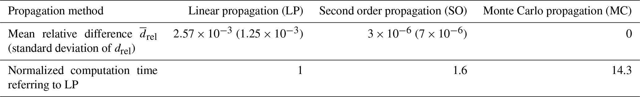
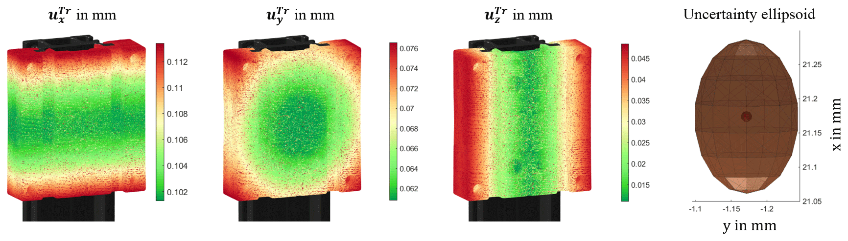
Figure 4 Uncertainty components ${\mathit{u}}_{\mathbf{x}}^{\mathbf{\text{Tr}}}$, ${\mathit{u}}_{\mathbf{y}}^{\mathbf{\text{Tr}}}$, and ${\mathit{u}}_{\mathbf{z}}^{\mathbf{\text{Tr}}}$ of the x, y, and z components, respectively (from left to right), and uncertainty ellipsoid for U_Pt (small red sphere) and U^Tr (large brown ellipsoid) around an arbitrarily selected point.

Figure 5 Uncertainty ${\mathit{u}}_{\mathbf{c}}^{\mathbf{\text{Tr}}}$ of the slider (a) and histogram of uncertainty components U_Pt, ${\mathit{u}}_{\mathbf{x}}^{\mathbf{\text{Tr}}}$, ${\mathit{u}}_{\mathbf{y}}^{\mathbf{\text{Tr}}}$, ${\mathit{u}}_{\mathbf{z}}^{\mathbf{\text{Tr}}}$, and ${\mathit{u}}_{\mathbf{c}}^{\mathbf{\text{Tr}}}$ (b).

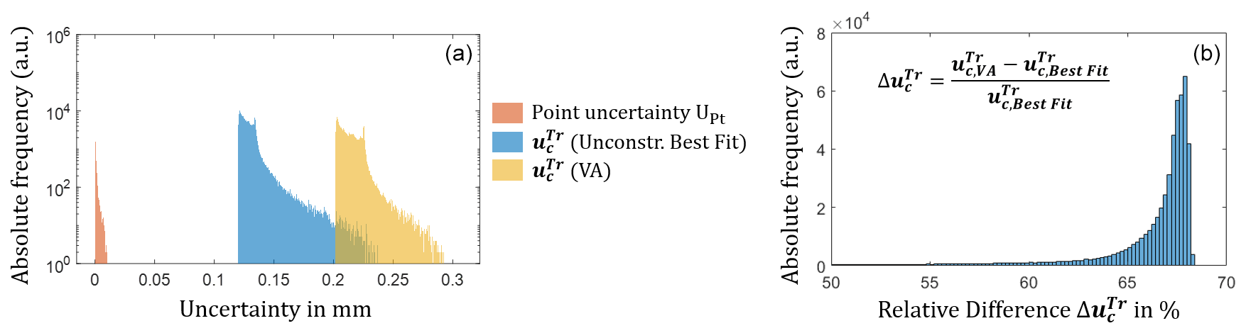
Figure 6 Histogram of the initial uncertainty U_Pt and propagated uncertainty ${\mathit{u}}_{\mathbf{c}}^{\mathbf{\text{Tr}}}$ for VA and the unconstrained (unconstr.) Gaussian best fit (a). Histogram of relative differences $\mathbf{\Delta }{\mathit{u}}_{\mathbf{c}}^{\mathbf{\text{Tr}}}$ between VA and unconstrained Gaussian best fit (b).

The linear propagation (LP) is valid for small rotations due to the small angle approximation, where sin x≈x and cos x≈1 for small values of x. Due to a preceding rough alignment, rotations smaller than 0.01 rad ($\approx \mathrm{0.6}{}^{\circ }$) are determined by VA, resulting in relative errors of $\mathrm{1.7}\times {\mathrm{10}}^{-\mathrm{5}}$ for the sine function and $\mathrm{5}\times {\mathrm{10}}^{-\mathrm{5}}$ for the cosine function. To assess the effect of possible approximation errors, the results for the LP are compared to the propagation results for the second order (SO) and the Monte Carlo (MC) propagation. For this purpose, the propagation methods implemented in the UncLib library in MATLAB R2018b supplied by Wollensack (2020) were used.

4 Discussion

Figure 3 shows the coordinate system (CS) orientation and the datum of A and B, respectively, that define the assembly. The CS position is centered in the barycenter of the slider. Each point p_2,i in P₂ is rotated around the CS origin ${\mathbf{p}}_{\mathrm{0}}(\mathrm{0}\mid \mathrm{0}\mid \mathrm{0})$, with a radius r_i, which is defined as the Euclidean distance of the point and origin, according to the following:

$$\begin{array}{}\text{(17)}& r_i={∥{\mathbf{p}}_{\mathrm{2},\mathbf{i}}-{\mathbf{p}}_{\mathrm{0}}∥}_{\mathrm{2}}.\end{array}$$

Due to the contribution of the transformation uncertainty u_T to the transformation, the propagated uncertainty U^Tr increases with an increasing radius r, which can be related by analyzing the visualizations in Fig. 4, where the components ${\mathit{u}}_{\mathbf{x}}^{\mathbf{\text{Tr}}}$, ${\mathit{u}}_{\mathbf{y}}^{\mathbf{\text{Tr}}}$, and ${\mathit{u}}_{\mathbf{z}}^{\mathbf{\text{Tr}}}$ increase towards the corners of the analyzed slider. The uncertainties of rotational transformation parameters cause parabolic and circular patterns for the propagated uncertainties. Here, a large uncertainty u_Θ of the rotation in Θ causes a large uncertainty ${\mathit{u}}_{\mathbf{x}}^{\mathbf{\text{Tr}}}$. The components ${\mathit{u}}_{\mathbf{y}}^{\mathbf{\text{Tr}}}$ and ${\mathit{u}}_{\mathbf{z}}^{\mathbf{\text{Tr}}}$ are affected to a smaller extent by u_ϕ and u_ψ, respectively. The uncertainties u_T,x, u_T,y, and u_T,z cause an offset to ${\mathit{u}}_{\mathbf{x}}^{\mathbf{\text{Tr}}}$, ${\mathit{u}}_{\mathbf{y}}^{\mathbf{\text{Tr}}}$, and ${\mathit{u}}_{\mathbf{z}}^{\mathbf{\text{Tr}}}$, respectively. The datum A (see Fig. 3) constraining the x translation shows the largest propagated uncertainty ${\mathit{u}}_{\mathbf{x}}^{\mathbf{\text{Tr}}}$ of about 0.1 mm. The uncertainty ${\mathit{u}}_{\mathbf{y}}^{\mathbf{\text{Tr}}}$ of about 0.06 mm, associated to datum B and constraining the y direction, is nearly half as large. The uncertainty ${\mathit{u}}_{\mathbf{z}}^{\mathbf{\text{Tr}}}$ in the z direction is about 0.01 mm, which matches the initial uncertainty before propagation, since t_z is constrained to zero. The fact that ${\mathit{u}}_{\mathbf{x}}^{\mathbf{\text{Tr}}}$ is about 2 times the magnitude of ${\mathit{u}}_{\mathbf{y}}^{\mathbf{\text{Tr}}}$ might be an effect of imbalanced point sets because datum B contains about half the points of datum A. Due to a high uncertainty ${\mathit{u}}_{\mathbf{x}}^{\mathbf{\text{Tr}}}$, the projection of the uncertainty ellipsoid shown in Fig. 4 in the x–y plane is distorted in the x direction. If no rough pre-alignment is performed before VA, an increase in the uncertainty ${\mathit{u}}_{\mathbf{c}}^{\mathbf{\text{Tr}}}$ of about a factor of 10 is observed because the optimization result converges poorly for the equal termination criteria. This emphasizes the need for a sufficient pre-alignment. By comparing the uncertainty ${\mathit{u}}_{\mathbf{c}}^{\mathbf{\text{Tr}}}$ for the VA algorithm to an unconstrained Gaussian best fit registration, an increase in ${\mathit{u}}_{\mathbf{c}}^{\mathbf{\text{Tr}}}$ of about 50 % to 68 % was observed, as shown in Fig. 6. Hence, the VA algorithm results in approximately twice the measurement uncertainty. The mean relative differences are as follows:

$$\begin{array}{}\text{(18)}& {\stackrel{\mathrm{‾}}{d}}_{\text{rel}}=\text{mean}\left({\displaystyle \frac{{\mathit{u}}_{\mathbf{c}}^{\mathbf{\text{Tr}}}-{\mathit{u}}_{\mathbf{c},\mathbf{\text{MC}}}^{\mathbf{\text{Tr}}}}{{\mathit{u}}_{\mathbf{c},\mathbf{\text{MC}}}^{\mathbf{\text{Tr}}}}}.\right)\end{array}$$

For the LP and SO propagation methods referring to the MC propagated uncertainty ${\mathit{u}}_{\mathbf{c},\mathbf{\text{MC}}}^{\mathbf{\text{Tr}}}$ are presented in Table 1. According to ISO/IEC (2008a), the MC method should be used when a linearization of the propagation function is inadequate and, therefore, is considered as the ground truth method. The propagated distribution is gathered due to propagating a large number of random samples (here 10⁶ samples) through the model function. For both the LP and SO propagation, the values of ${\stackrel{\mathrm{‾}}{d}}_{\text{rel}}$ are negligibly small, so that no significant variation in ${\mathit{u}}_{\mathbf{c}}^{\mathbf{\text{Tr}}}$ was observed. For a median propagated uncertainty ${\stackrel{\mathrm{̃}}{u}}^{\text{Tr}}$ of approximately 0.25 mm, the relative difference of $\mathrm{2.57}\times {\mathrm{10}}^{-\mathrm{3}}$ for the LP propagation results in an absolute error of approximately ±0.7 µm only. However, relative to the LP propagation, the computational cost for the MC propagation is about 14.3 times higher, while the factor of the SO propagation is merely about 1.6.

5 Conclusion and outlook

The main contribution to the propagated uncertainty is due to the uncertainty in the transformation parameters u_T, which depend on the formulation of the registration problem. Confirming the work of Galovska et al. (2012), it was shown that the number and arrangement of the reference points considered for registration strongly influence the propagated uncertainty. By an unconstrained Gaussian best fit, all points are weighted equally, which reduces the uncertainty compared to the VA algorithm, where certain points are considered in the constraint function. Thus, compared to the unconstrained Gaussian best fit, the uncertainty is nearly doubled. A preceding rough alignment helps to strongly reduce the propagated uncertainty. Due to small transformations remaining for the VA after pre-alignment, the small angle approximation and, hence, a linear propagation model can be sufficiently applied. The propagated uncertainties are relatively large. The main contribution to the propagated uncertainty U^Tr is the uncertainty of transformation u_T. Large observed values for u_T are also assumed to be caused due to large values for the delta transformation δT. Since, in practice, no random shift of the point set to register occurs, for practical measurements the uncertainty of transformation u_T and the propagated uncertainty U^Tr are assumed to be considerably smaller. As an outlook, the propagation model can be prospectively used to state uncertainties for virtual measurements that are performed on the registered data sets. Here the analysis of the gap flush between the taillight and tailgate for an automotive application by virtual measurements regarding uncertainties is to mention Galovska et al. (2018). Parameter studies on best termination criteria can be performed, aiming to minimize the uncertainty of transformation u_T.

The propagation model can be verified by analyzing repeatability studies on virtual measurements of registered assemblies. Moreover, computationally efficient minimum variance estimators, such as Kalman filters can be studied in order to evaluate the preliminary VA registration result during an iteration based on the magnitude of uncertainty. As a further approach, the Jacobian matrix J of the uncertainty propagation can be evaluated during the VA optimization, which is a measure for the sensitivity of the propagated uncertainty towards the transformation variables. By doing so, fewer uncertain registration results can possibly be determined.