Iterative feature detection of a coded checkerboard target for the geometric calibration of infrared cameras

The geometric calibration of cameras becomes necessary when images should be undistorted, geometric image information is needed or data from more than one camera have to be fused. This process is often done using a target with a checkerboard or circular pattern and a given geometry. In this work, a coded checkerboard target for thermal imaging cameras and the corresponding image processing algorithm for iterative feature detection are presented. It is shown that, due in particular to the resulting better feature detectability at image borders, lower uncertainties in the estimation of the distortion parameters are achieved.

1 Introduction

Infrared (IR) cameras (also called thermal imaging cameras) are widely used to perform temperature field measurements by detecting the IR radiation emitted by object surfaces. The correlation between the detected radiation flux and the international temperature scale ITS-90 is obtained through a radiometric calibration (König et al., 2020). In addition, just as for cameras that work in the visible (VIS) spectral range, there is the possibility of a geometric calibration (Luhmann et al., 2013). This additional calibration is required to compensate for image distortion (intrinsic calibration), to obtain geometric information from the images (also intrinsic calibration) or to determine the relationships between multiple camera coordinate systems as part of a sensor data fusion process (extrinsic calibration).

For this purpose, images of so-called calibration targets with known geometric dimensions are used. The positions of the target features in the images are detected in a first step. The calibration parameters of a camera model are estimated so that the calculated Euclidean distances between the features correspond as closely as possible to the target dimensions. One problem with commonly used uncoded targets (those with a checkerboard or circular pattern) is that the entire target and parts of its border must always be completely visible in the camera images. This is a limitation in situations with small fields of view (FOV) (e.g., when only small parts of the image overlap during the extrinsic calibration of a multicamera system; Rangel et al., 2021) and when features should be placed near the image borders. This aspect is crucial in any geometric calibration: it will be shown in the course of this work (Sect. 5) that these features near the image border have a strong effect on the uncertainty in the camera's radial distortion parameters. The target and its algorithmic evaluation presented in this work are intended to address this problem. Iterative feature detection in combination with the presented actively heated calibration target can thereby reduce the calibration uncertainty compared to the state of the art.

In this paper, the basic principles of calibration are presented first, along with related works (see Sect. 2). Subsequently, the proposed method is described, whereby the target design and the iterative calibration algorithm are discussed (see Sect. 3). The results obtained when the target was parameterized and compared experimentally with an uncoded checkerboard target are then described (see Sect. 4). Finally, the results are discussed (see Sect. 5), and a summary and outlook are given (see Sect. 6).

2 Fundamentals

In the following, the basic principles of a geometric calibration will be briefly discussed, with special attention paid to the determination of the distortion parameters. Subsequently, the state of the art regarding coded and uncoded calibration targets for IR cameras used in related works is presented.

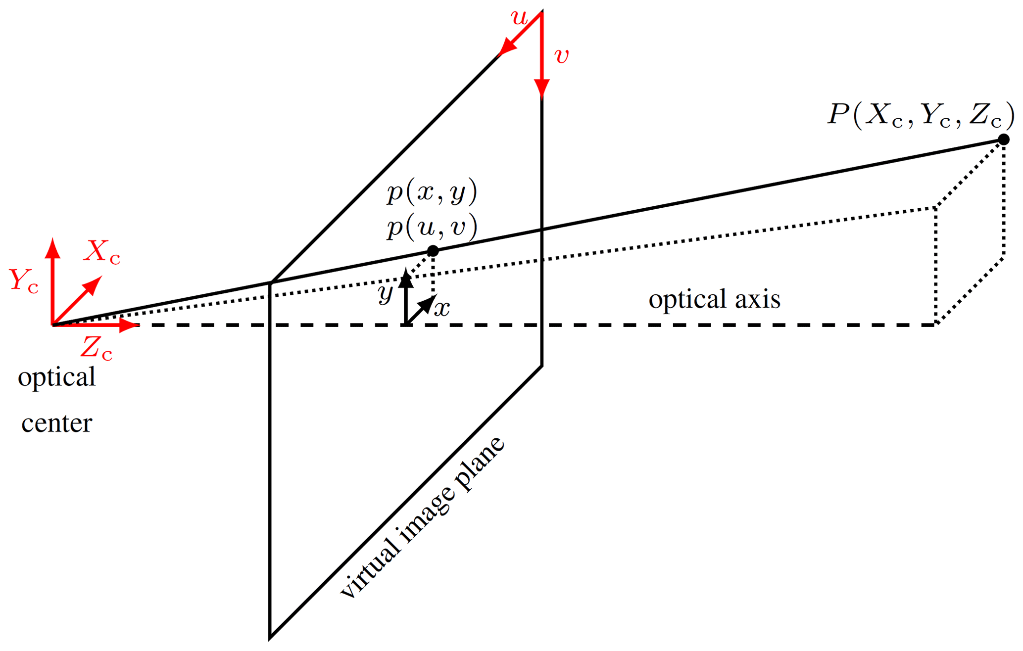
Figure 1 Relationship between a 3D point $P(X_{\mathrm{c}},Y_{\mathrm{c}},Z_{\mathrm{c}})$ and an image point p(u,v) in the pinhole camera model with a virtual image plane; based on Ordoñez Müller (2018).

2.1 Calibration

The parameters to be determined with an intrinsic geometric camera calibration are composed of the camera matrix K and the distortion coefficients k. The following camera matrix K contains the components of the idealized pinhole camera model, which maps a 3D point $P(X_{\mathrm{c}},Y_{\mathrm{c}},Z_{\mathrm{c}})$ in the camera coordinate system onto the 2D image plane of the camera at point p(u,v) (see Fig. 1) if the detector elements are quadratic (Szeliski, 2010):

$$\begin{array}{}\text{(1)}& \left[\begin{array}{c}u\\ v\\ \mathrm{1}\end{array}\right]={\displaystyle \frac{\mathrm{1}}{Z_{\mathrm{c}}}}\underset{\mathbf{K}}{\underbrace{\left[\begin{array}{ccc}{f}_{\mathrm{u}}& \mathrm{0}& c_{\mathrm{u}}\\ \mathrm{0}& f_{\mathrm{v}}& c_{\mathrm{v}}\\ \mathrm{0}& \mathrm{0}& \mathrm{1}\end{array}\right]}}\left[\begin{array}{c}{X}_{\mathrm{c}}\\ Y_{\mathrm{c}}\\ Z_{\mathrm{c}}\end{array}\right].\end{array}$$

Here, f_u and f_v are the focal lengths in units of px, and c_u and c_v are the distances between the point of intersection of the camera axis with the imaging plane and the upper left corner of the image (also in units of px). It should be noted that, to make the unit px describable in the SI system of units, the size of a px corresponds to the side length of a detector element (also called the pixel pitch; ≈17 µm for the long-wavelength infrared camera used here). However, because of the camera optics required, a perfect pinhole camera does not exist. The deviations that occur are described by distortion models; most commonly, the model of Brown (1971) is used:

$$\begin{array}{}\text{(2)}& \left[\begin{array}{c}{x}_{\mathrm{d},\mathrm{rad}}\\ y_{\mathrm{d},\mathrm{rad}}\end{array}\right]=(\mathrm{1}+k_{\mathrm{1}}{r}^{\mathrm{2}}+k_{\mathrm{2}}{r}^{\mathrm{4}}+k_{\mathrm{3}}{r}^{\mathrm{6}})\left[\begin{array}{c}x\\ y\end{array}\right]\end{array}$$

$$\begin{array}{}\text{(3)}& \left[\begin{array}{c}{x}_{\mathrm{d},\tan }\\ y_{\mathrm{d},\tan }\end{array}\right]=\left[\begin{array}{c}x+(\mathrm{2}{p}_{\mathrm{1}}xy+p_{\mathrm{2}}(r^{\mathrm{2}}+\mathrm{2}{x}^{\mathrm{2}}\left)\right)\\ y+(\mathrm{2}{p}_{\mathrm{2}}xy+p_{\mathrm{1}}(r^{\mathrm{2}}+\mathrm{2}{y}^{\mathrm{2}}\left)\right)\end{array}\right]\end{array}$$

with

$$\begin{array}{}\text{(4)}& r^{\mathrm{2}}=x^{\mathrm{2}}+y^{\mathrm{2}},\end{array}$$

where x and y are the undistorted image positions w.r.t. the principal point (in the camera, not the image coordinate system: $x=u-c_{\mathrm{u}},y=v-c_{\mathrm{v}}$), x_d,rad and y_d,rad are the image positions with radial distortion, x_d,tan and y_d,tan are the image positions with tangential distortion, and $\mathit{k}={\left[k_{\mathrm{1}},k_{\mathrm{2}},k_{\mathrm{3}},p_{\mathrm{1}},p_{\mathrm{2}}\right]}^{\mathrm{T}}$ are the model distortion coefficients to be determined. The distortion corresponds to a local scale change. In the case of radial distortion, this change depends on the distance r to the principal point and is caused by the nonsymmetrical placement of the lens in front of (pincushion distortion, k₁>0) or behind (barrel distortion, k₁<0) the aperture and the spherical shape of the lenses (Luhmann et al., 2020). Tangential distortion occurs primarily due to errors in the alignment of the optical components with each other (Luhmann et al., 2020).

The nine parameters in K and k are optimized using the algorithm of Zhang (2000). Therefore, points on a planar target in several (at least four) image poses are needed as input variables. The cost function of the nonlinear optimization is based on minimizing the total Euclidean distance (RMSE, reprojection error) between the given points and their reprojection. Schramm et al. (2021) show that the uncertainty in the calibration depends on the uncertainty in the reference data, i.e., the quality of the feature localization.

2.2 Related works

The use of different targets for the geometric calibration of IR cameras is the subject of various publications. In the vast majority, uncoded targets are used, which are usually based on the detection of a circle or checkerboard (Soldan et al., 2011). Features are mostly created by generating a contrast in emissivity, such as that achieved by applying paint on aluminum (Lagüela et al., 2011) or copper (Kim et al., 2015), or by making holes in a high-emissivity material with a low-emissivity plate behind (Ordoñez Müller, 2018). These types of targets are heated to generate an image contrast (see Sect. 3.1). There are also works in which the target is cooled to reduce the influence of interfering radiation (Herrmann et al., 2020). Furthermore, targets where the features are maintained at a different temperature (by active heat sources such as light bulbs or LEDs) from the rest of the target are also used (Beauvisage and Aouf, 2017). These targets often achieve very good results in the long-wavelength infrared (LWIR) and mid-wavelength infrared (MWIR) due to their high contrast compared to emissivity-based targets, but they require a complex setup and are thus more expensive and heavier. Also, the results of extrinsic calibrations with VIS cameras are worse (Schramm et al., 2021). Thus, the question arises of how to improve the calibration quality of classical emissivity-based targets compared to the state of the art.

The use of coded targets is much rarer. Coded features are used in Lagüela et al. (2011), Luhmann et al. (2013) and Schmidt and Frommel (2015) in combination with circular targets. In Lagüela et al. (2011) and Schmidt and Frommel (2015), this is primarily necessary to ensure a unique allocation due to the symmetry of circle features. The disadvantage of these circle targets is that the complete circle must always be visible for correct detection and localization. As a consequence, the placement of features close to the image edge depends on the circle radius. This leads to a trade-off: larger circles allow a more precise centroid calculation, but at the same time they increase the distance to the image edge.

Coded markers such as the ArUco markers (Romero-Ramirez et al., 2018) proposed here are also used for the calibration of IR cameras. In de Oliveira et al. (2016), a multispectral camera (VIS to near-infrared, NIR) is calibrated using ArUco, but the markers are placed on a 3D instead of a 2D target. Calibration with ArUco marker corners as data points is not recommended due to the limited corner detection accuracy of the ArUco algorithm. Therefore, in the often-used OpenCV framework, an own target design (ChArUco) is proposed. There, the ArUco markers are integrated into the white squares of the chessboard. All ArUco markers surrounding a checkerboard field must be detected, which again negatively affects the positionability at the image edges. In Aalerud et al. (2019), the intrinsic parameters of NIR sensors are determined with an uncoded checkerboard, but an extrinsic pose estimation is performed with ArUco and specially developed retroreflective markers. Also, in Lin et al. (2019), ArUco is used for pose estimation with an NIR-sensitive camera. There are clear differences between the NIR and LWIR ranges in both the camera technology and the object radiation (reflection of external radiation compared to own temperature radiation).

A combination of AprilTag markers and a checkerboard for camera calibration in the LWIR spectral range is described in Choinowski et al. (2019). Five AprilTag markers are distributed on the checkerboard pattern and placed in such a way that they replace individual black squares of the checkerboard. The algorithm used to detect the corners (Wohlfeil et al., 2019) also differs from the algorithm proposed here (see Sect. 3.2). In that work, all corners appearing in the image are initially found using a corner extractor and filtered according to whether the surroundings of the corner include the four black-to-white transitions of a checkerboard corner. The required radius of the surroundings of the corner in this step (up to 6.5 px) limits the search for potential points at the edge of the image. Unfortunately the authors do not describe how they address this issue. Afterwards, the homography determined by the AprilTag is used to calculate where the corners should be positioned on the target, and the remaining corner points are selected and assigned. Since the same LWIR camera (and lens) is used in Choinowski et al. (2019), the results can be compared to some extent (see Sect. 4.3).

Furthermore, coded targets are used in the VIS spectral range. Besides the ChArUco approach mentioned above, Schops et al. (2020) and the coded target used in the OpenCV library based on the work of Duda and Frese (2018) (unknown handling of a coded feature) should be mentioned here. In Schops et al. (2020), the calculated homography of an AprilTag is used, and the expected target feature positions are refined by a cost function that penalizes the gray value asymmetry in the symmetric target homography. Unlike the solution from Choinowski et al. (2019), a comparison with that from Schops et al. (2020) is not feasible because a global camera parameter model is not used in that work (compare to Sect.  2.1), and, besides the algorithm, the holistic design of the target is a crucial influence on the calibration quality of IR cameras (see Sect. 3.1 and the discussion in Sect.  5). A similar iterative algorithm approach to that presented in this work but for the calibration of VIS cameras has not been reported.

None of the related works report a full solution for the detection of features close to the image edges by infrared cameras and how this affects the calibration. For this reason, a novel method involving iterative feature detection (see Sect. 3.2) in the full image region is proposed in this work. Combined with an actively heated target (see Sect. 3.1), the present approach should circumvent the limitations described above. Experiments (see Sect. 4) demonstrate that the present method allows improved boundary detection and reduces uncertainty in the geometric calibration.

3 Approach

In this section, the target and the feature detection algorithm are presented. The algorithm, a data set used in Sect. 4 and a target template are available online.¹

Figure 2 Examples of images of the proposed ArUco coded checkerboard target.

3.1 Target design

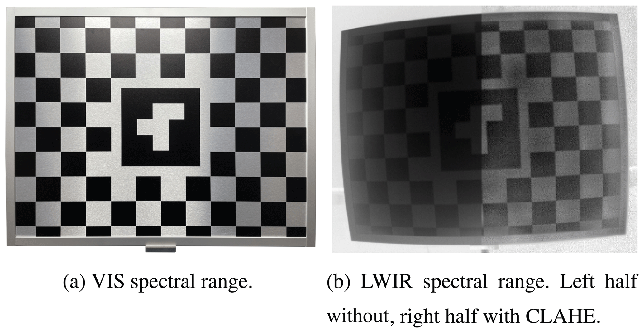
The target used in the present work has a centered ArUco marker (Romero-Ramirez et al., 2018) framed by a checkerboard pattern (see Fig. 2). The sizes of the target and the features have a crucial impact on the detection. The optimal checkerboard target size in relation to the camera's FOV is discussed in Schramm et al. (2021). The size of the centered ArUco marker is also a trade-off. On the one hand, increasing the size of the marker increases the relative resolution of the marker in the image and thus the detectability and accuracy of the pose estimation. However, increasing the number of squares of the checkerboard background that the marker extends over decreases the number of data points, and the data points are used to optimize the final calibration parameters.

For better comparability with the uncoded checkerboard target from Schramm et al. (2021), the same target dimensions (600 mm×450 mm) and checkerboard side lengths (50 mm) were used in the present work. This meant that a white border and full-length checkerboard squares at the target border were not needed for detection, allowing another line of checkerboard corners to be used at the outermost edge. At the same time, 23 features in the center were replaced by the ArUco marker. The total number of checkerboard corners in the coded target was 76. This is more than in the uncoded checkerboard target (54), but all features of an uncoded target must always be visible. In contrast, in the images of the coded target, a number of the features were often outside the image field. Since only one ArUco marker was needed, with individual elements that should be as large as possible, a marker with a coarse 3×3 dictionary was selected (ID=1). The edge length of the marker was 160 mm. The size was chosen based on the camera used (see Sect. 4) and the maximum calibration distance of 2 m, which resulted in an ArUco marker block length of $\approx \mathrm{7}\mathrm{px}\times \mathrm{7}\mathrm{px}$. The value decreased when the target was rotated relative to the image plane. ArUco marker detection was performed without any problems in the experiments described in Sect. 4.

To detect these features using an LWIR camera, they were printed on an Alu-Dibond plate with a heated back (achieved using a self-adhesive, electrical heating foil manufactured by Thermo Technologies). Alu-Dibond plates have the advantage that they can be ordered very easily and inexpensively from many online printing companies as wall posters. The complete target (plate, heating mat and custom-made frame) weighed less than 1.8 kg.

The gray value U_cam of an image pixel is obtained according to the radiometric chain from the emissivity of the measurement spot ε as well as the corresponding temperature-dependent gray values $U_{\mathrm{obj}}^{\mathrm{BB}}$ and $U_{\mathrm{amb}}^{\mathrm{BB}}$ of an object and the environment using the black body assumption:

$$\begin{array}{}\text{(5)}& U_{\mathrm{cam}}=\mathit{\epsilon }{U}_{\mathrm{obj}}^{\mathrm{BB}}-\left(\mathrm{1}-\mathit{\epsilon }\right)U_{\mathrm{amb}}^{\mathrm{BB}}.\end{array}$$

The relationship between the black body equivalent gray value $U_{\mathrm{obj}}^{\mathrm{BB}}$ and the object temperature T_obj is determined during the radiometric calibration of the camera. If the target has two different surface types (painted and blank aluminum) with two different emissivities ε₁ and ε₂, this leads, according to Eq. (5), to a gray value contrast ($\mathrm{\Delta }U=U_{\mathrm{1}}-U_{\mathrm{2}}$) of

$$\begin{array}{}\text{(6)}& \mathrm{\Delta }U=\left(U_{\mathrm{target}}^{\mathrm{BB}}-U_{\mathrm{amb}}^{\mathrm{BB}}\right)\left({\mathit{\epsilon }}_{\mathrm{1}}-{\mathit{\epsilon }}_{\mathrm{2}}\right).\end{array}$$

To maximize the first part of the equation, the temperature difference must be large and/or the sensitivity of the camera (which affects the radiometric calibration parameters) must be high. This means, for example, that a much smaller temperature difference is required for feature detection using high-sensitivity MWIR cameras with InSb detectors than when using microbolometer LWIR cameras, given that a typical InSb (indium antimonide) MWIR camera is a factor of approx. 100 more sensitive (Vollmer and Möllmann, 2017). This difference is manifested in the heating foil required: while a heating foil with an electrical power density of $M=\mathrm{0.154}\mathrm{W}{\mathrm{m}}^{-\mathrm{1}}$ is sufficient for a typical MWIR camera (InfraTec ImageIR 8300 hp), a heating foil with an electrical power density of $M=\mathrm{41.8}\mathrm{W}{\mathrm{m}}^{-\mathrm{1}}$ is required to reach an adequate feature contrast when using an LWIR camera (Optris PI 450). Since an LWIR camera was considered in this work, the more powerful heating foil was used. It should be ensured that the size of the heating mat is similar to the size of the target, since a homogeneous temperature distribution on the front of the target supports the feature detection process. Due to the Dibond between the two aluminum layers, the temperature uniformity is not ideal. In the examined application, the temperatures at the target center and the target corners deviated from each other by less than 10 ^∘C. Instead of a heating foil, the target could also be placed on the ground outdoors (Choinowski et al., 2019) and the low self-radiation of the sky can be used as reflected ambient radiation, although this is done at the expense of operational flexibility.

To further increase the contrast and to reduce the influence of the nonuniform temperature distribution on the target surface, it is recommended that an adaptive contrast adjustment (CLAHE) should be performed (Pizer et al., 1987). Its parameters should be determined empirically for the particular data set by observing the detection rate. For the detection of the coded target with the camera used in this work, the parameters were set to $\mathtt{clipLimit}=\mathrm{5.0},\mathtt{tileGridSize}=(\mathrm{16},\mathrm{12})$. Even if the features are found without contrast enhancements, this preprocessing step can have a positive effect on the results and should therefore be considered.

Figure 3 Schematic process flow of the feature detection algorithm.

3.2 Feature detection and calibration algorithm

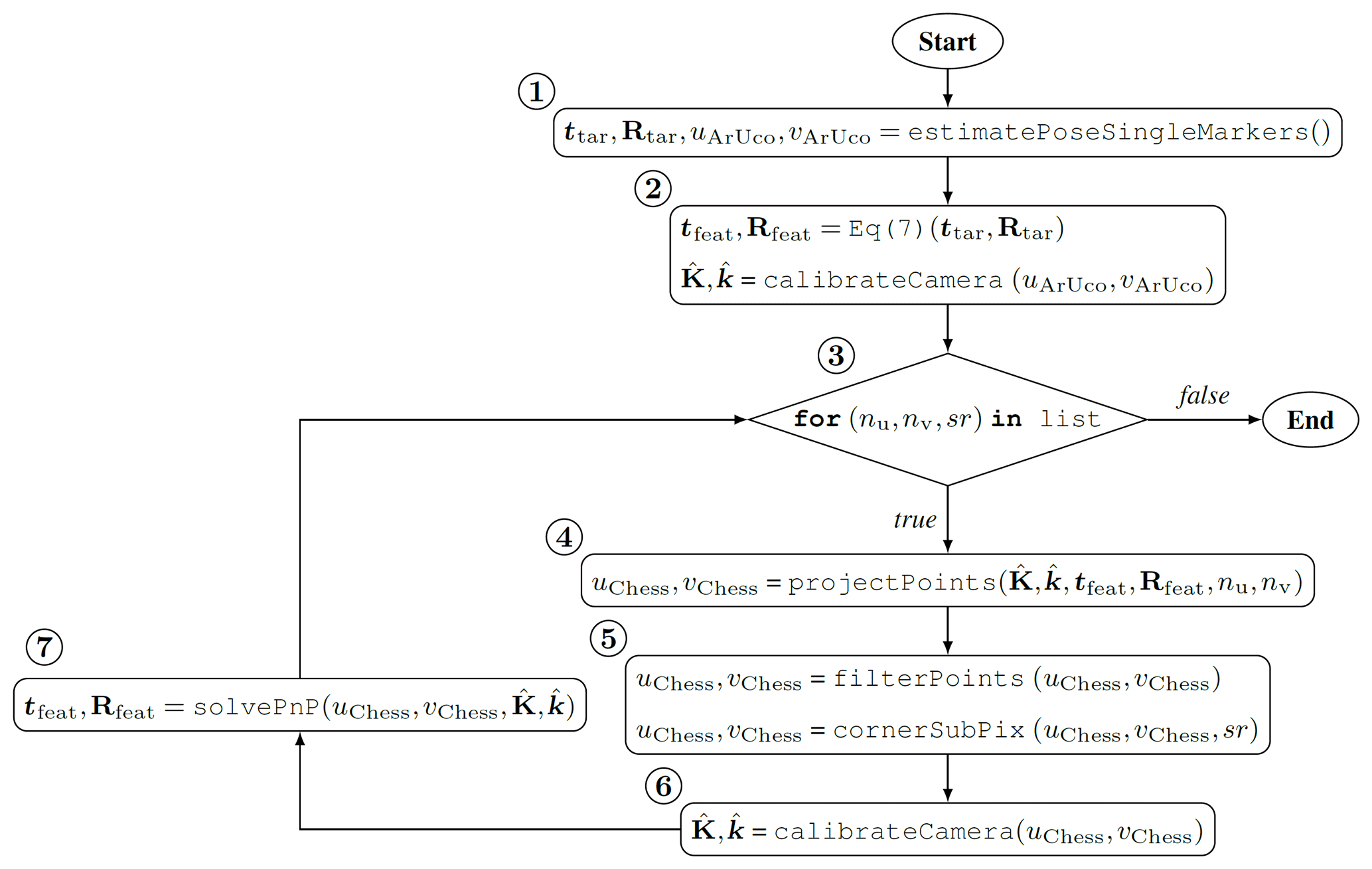
Since the final RMSE of a good calibration is below 1 px (and often in the range 0.1–0.4 px), the feature positions must also be found to the subpixel level. To find these features in such an accurate manner, an iterative calibration algorithm was implemented according to the schematic process flow shown in Fig. 3. The code was written in Python and was based on the functions of the OpenCV library (Bradski, 2000).

First, the ArUco markers of the image data set were detected (step 1). The 3D translations t_tar and rotations R_tar of the target center poses relative to the camera were estimated from the ArUco marker. The translations ${\mathit{t}}_{\mathrm{tar}\to \mathrm{feat},i}$ between each checkerboard corner i and the target center were given by the target design (as the target is planar, z=0 m). The position of a checkerboard corner in the camera coordinate frame was calculated via

$$\begin{array}{}\text{(7)}& {\mathit{t}}_{\mathrm{feat},i}={\mathit{t}}_{\mathrm{tar}}+{\mathbf{R}}_{\mathrm{tar}}\cdot {\mathit{t}}_{\mathrm{tar}\to \mathrm{feat},i}.\end{array}$$

Furthermore, an initial geometric calibration was performed by detecting the ArUco corners in all images (step 2). Using the function projectPoints, the 3D points ${\mathit{t}}_{\mathrm{cam}\to \mathrm{feat},i}$ were mapped to image coordinates (step 4). However, since ArUco corners can only be localized imprecisely (no subpixel refinement), the rotation and translation components and the initial calibration parameters contain large uncertainties. As a result, the deviation of the projected features increases significantly as a function of the distance to the target center (see Fig. 4a). Therefore, an iterative function was used to gradually increase the accuracy of the calibration. After the ArUco calibration, only the checkerboard features around the target center were evaluated, and the number of corner columns n_u and number of rows n_v were increased stepwise. At the same time, the search radius sr within which the corner positions were refined by OpenCV was reduced (step 3). The projected points from step 4 were then filtered (points outside the FOV were removed), and corner refinement was performed (step 5). Since this led to an increase in the precision of the feature positions (see Fig. 4b), the calibration parameters were re-estimated (step 6), and then required target poses were calculated using solvePnP (step 7). The algorithm iterated until the maximum number of features were used (n_u,n_v: the target feature grid size) and the search radius was minimized. The parameterization is discussed in Sect. 4.1.

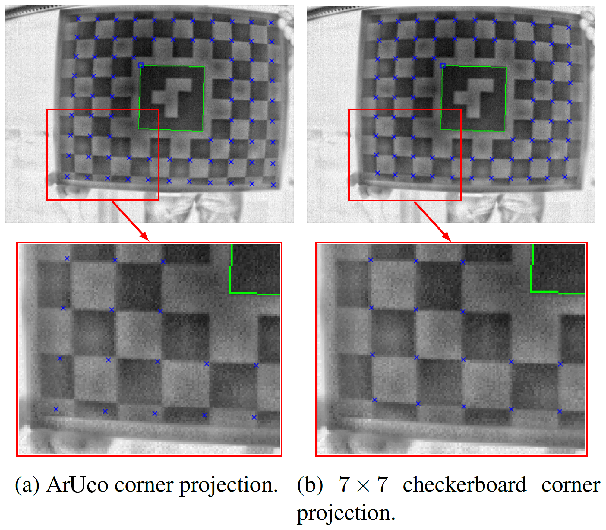
Figure 4 Increased projected corner precision after the initial calibration with an ArUco marker (a) and with the center 7×7 checkerboard corners (b).

4 Performed experiments

In this section, the experimental results from the coded target presented above and the uncoded checkerboard target from Schramm et al. (2021) are compared. In our experiments, an LWIR camera (Optris PI 450) was used, which is sensitive to radiation in the spectral range from 7.5 to 13 µm. Its resolution of 382 px×288 px is low compared to common VIS cameras. This camera has a wide-angle lens with an FOV of $\mathrm{53}{}^{\circ }\times \mathrm{38}{}^{\circ }$.

For the experiments, 60 images of each target were acquired. After switching on the heating foils, it was necessary to wait for about 15 min for the plates to reach thermal stationarity. To make the underlying optimization problem solvable, it was important to change the target pose (the target position in the image and the rotation of the target) from image to image. Instead of performing a single calibration with all 60 images, a multicalibration was performed with M subsets of N images. While multicalibration is more common in the photogrammetry community (Luhmann et al., 2013; Wohlfeil et al., 2019) than in the computer vision community, an advantage of it is that statistical parameters such as the standard deviation can be calculated and outliers can be excluded. For a recorded data set, the standard deviation can be used to assess the quality of a calibration in terms of parameter uncertainty. This provides another quality measure beyond the reprojection error RMSE, whose absolute value depends on the camera characteristics. Outliers can be treated using the RMSE percentiles. If the subset's RMSE is significantly higher than the mean RMSE, it can be assumed that the subset is not suitable for calibration because, for example, images with similar target poses were selected from the data set. If the RMSE exceeds the relative measure of the selected percentile, the calibration parameters of the subset are not included in the calculation of the mean μ and the standard deviation σ. For each of the results presented below, information on whether the limit was set and, if so, the value at which it was set is provided in each case.

4.1 Parameterization

The parameterization effects of the number of checkerboard feature rows n_u, n_v as well as the search radius sr on the calibration results were then examined. The results were based on an obtained data set consisting of 60 images (the maximum number of images is not important negligible as long as it is significantly greater than the number of images per subset N).

Admissible values for the number of feature rows were odd and ranged between one frame around the ArUco marker and the maximum target dimensions $n_{\mathrm{u}}=\left\{\mathrm{7},\mathrm{9},\mathrm{11}\right\}$, $n_{\mathrm{v}}=\left\{\mathrm{7},\mathrm{9}\right\}$. As can be seen in Fig. 4, the minimum values (7×7) should be chosen for the first run. If larger values are used, features may be placed in other corners if the search radii are too large. This leads to wrong calibration parameters, which will project the corners to false positions in the next iteration step. The search radius sr must be selected such that the corner to be found is always present within the radius but adjacent checkerboard corners are not. By iteratively improving the projection of the features, the search radius can be reduced as the number of iteration steps increases. The best results are achieved when the search radius ends at its minimum value sr =1. If a corner is not refined by CornerSubPix (e.g., due to noise), the influence of mislocalization can be limited to the search radius. An example of wrong corner refinement due to wrong parameters is shown in Fig. 5. If the smallest number of features is used, it is possible to use all features with a smaller search radius, since the reprojection improves significantly in the first step (see Fig.  4). The maximum search radius should be smaller than half of the smallest recorded width or height (in px) of a checkerboard side length to avoid false assignments.

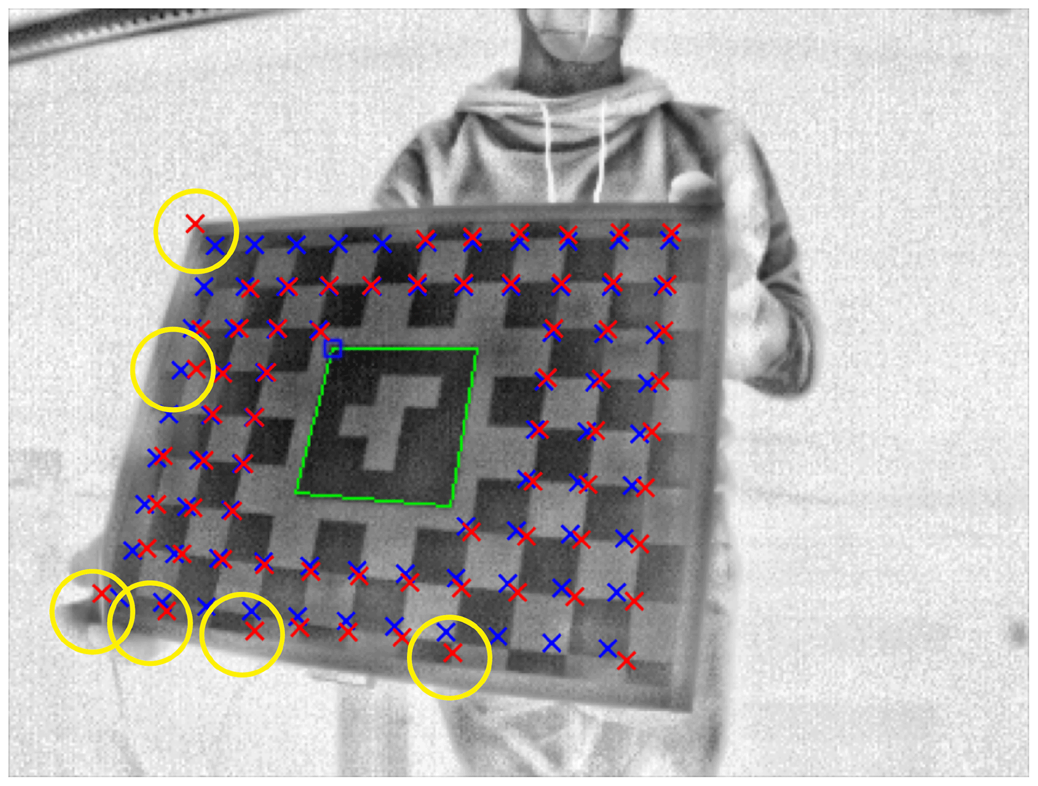
Figure 5 Incorrectly refined corners (yellow circles) due to the direct use of all target features in the first iteration step (n_u=11, n_v=9). Reprojected corners in blue, refined corners in red.

To test the parameterization, four different test scenarios were examined (see Table 1). In Scenario 1, four iteration steps were performed according to the description. In Scenario 2, the test was terminated at a minimum search radius of sr =2. In Scenario 3, all existing target checkerboard features were used directly after the ArUco step. In Scenario 4, a larger initial search radius was used.

Table 1 Test scenarios for the parameterization of n_u, n_v and sr.

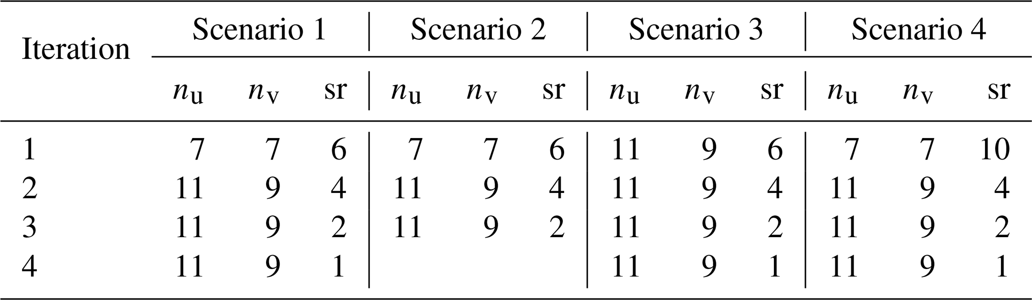
Figure 6 RMSE histograms resulting from the utilization of the different parameter sets in Table 1 for the multicalibration of N=15, M=10 000 without data filtering. The red line indicates the mean and the blue line the median value. The x axis is limited to 0.5 px to allow better visualization of the distribution; the truncated maximum values are max(RMSE_S1)=0.59 px, max(RMSE_S2)=0.98 px, max(RMSE_S3)=0.82 px and max(RMSE_S4)=4.21 px. Due to the presence of a few comparatively large outliers in Scenario 4, the mean value deviates significantly from the median.

As can be seen in Fig. 6, the median, the mean and the scatter of the RMSE were lowest for the parameter set of Scenario 1. The results of Scenario 3 did not differ much from those of Scenario 1, implying that the search radius sr has a greater influence on the result than the number of feature columns and rows n_u and n_v. Even though the basic influence of the parameterization is shown here, it should be noted that the specific parameters to use depend in particular on the side length of a checkerboard square.

4.2 Minimal border distance

To determine the extent to which the detection ability is increased at image borders, the uncoded checkerboard target and the coded target were mounted on a linear drive and moved out of the camera's FOV at a speed of less than 1 px per image. The last image in which the outermost corner was detected is shown in Fig. 7. The minimal border distance d_b was 8.5 px for the uncoded target and 1.6 px for the coded target. The influence of this characteristic on the distortion precision (Sect. 4.3) is discussed in Sect.  5.

Figure 7 Smallest border distance at which features are detected.

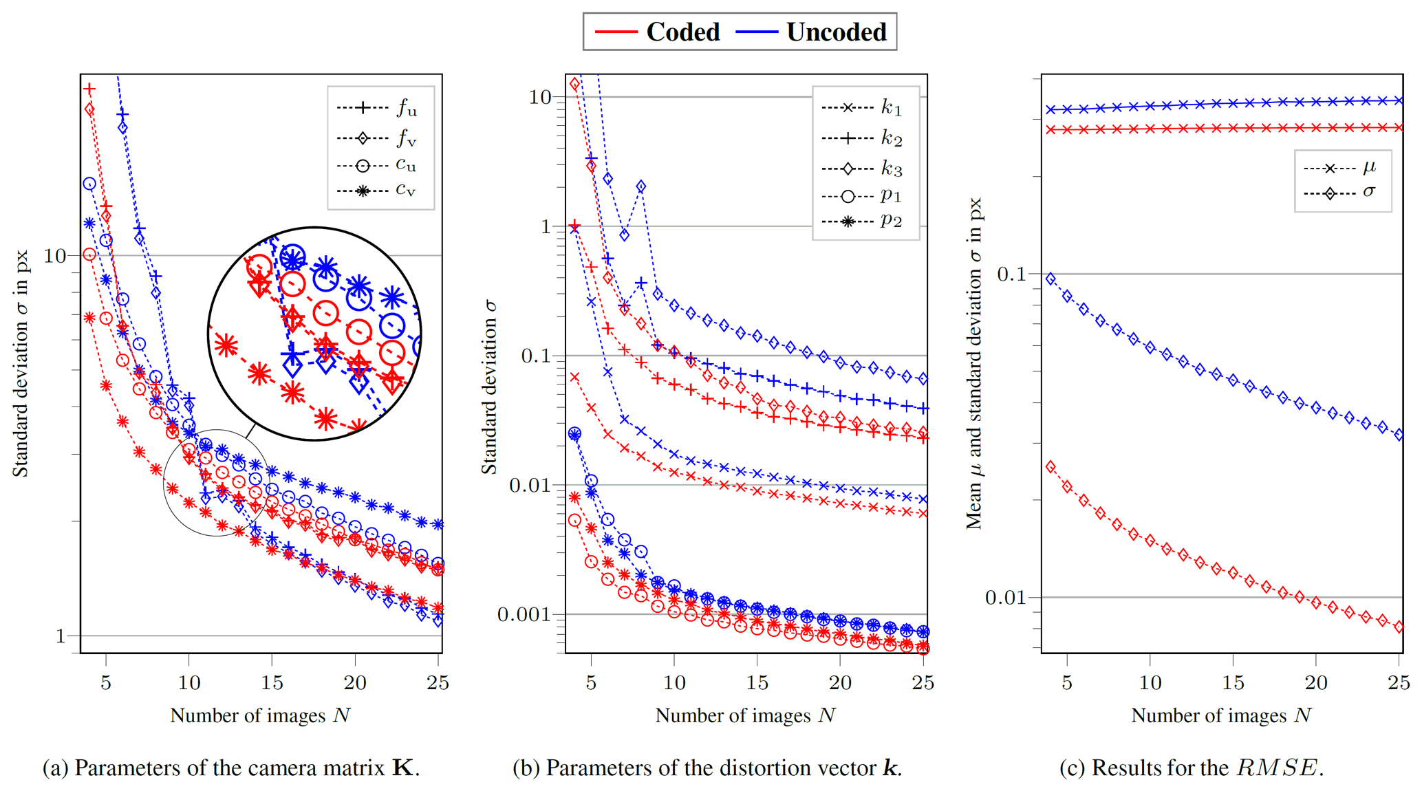
Figure 8 Logarithmic plots of the individual calibration parameter standard deviations σ (a, b) and the resulting RMSE standard deviation σ and mean value μ (c) as functions of the number N of images per subset for M=10 000 calibration runs and RMSE filtering at the 90th percentile. To improve visualization of the trends in the data shown, high values for the uncoded target at small N (e.g. $\mathit{\sigma }(f_{\mathrm{v}},N=\mathrm{4})=\mathrm{143.3}$, $\mathit{\sigma }(k_{\mathrm{3}},N=\mathrm{4})=\mathrm{1071}$) were truncated.

4.3 Distortion precision

First, the relationship of the precision (standard deviation) of each calibration parameter to the number of images per calibration N was examined. To remove outliers from the data, only calibration runs with an RMSE within its 90^th percentile were included in the analysis. Figure 8a and b show the results for the camera matrix parameters K (see Eq. 1) and the distortion parameters k (see Eqs. 2 and 3), respectively. As expected, the uncertainty in a parameter estimate decreased with the number of data points. For all distortion parameters and for the center point distances c_u and c_v, the parameter uncertainty was lower when the coded target was evaluated. The uncertainty was only lower with the uncoded target for the scaling factors f_u and f_v when N≥11. This was also reflected in the RMSE and its standard deviation (see Fig. 8c). For each N, calibration with the coded target led to better results. The mean RMSE over all numbers of images was 0.282 px for the coded target (with a mean standard deviation of 0.013 px) and 0.334 px for the uncoded target (with a mean standard deviation of 0.053 px).

Table 2 Results of the intrinsic camera calibrations with N=20, M=1000 and no percentile filtering. CH: values from the data set sep₂₀ in Choinowski et al. (2019); not comp.: mean value μ is not comparable due to manufacturing tolerances and potentially different focus settings. The best values for each parameter are shown in bold.

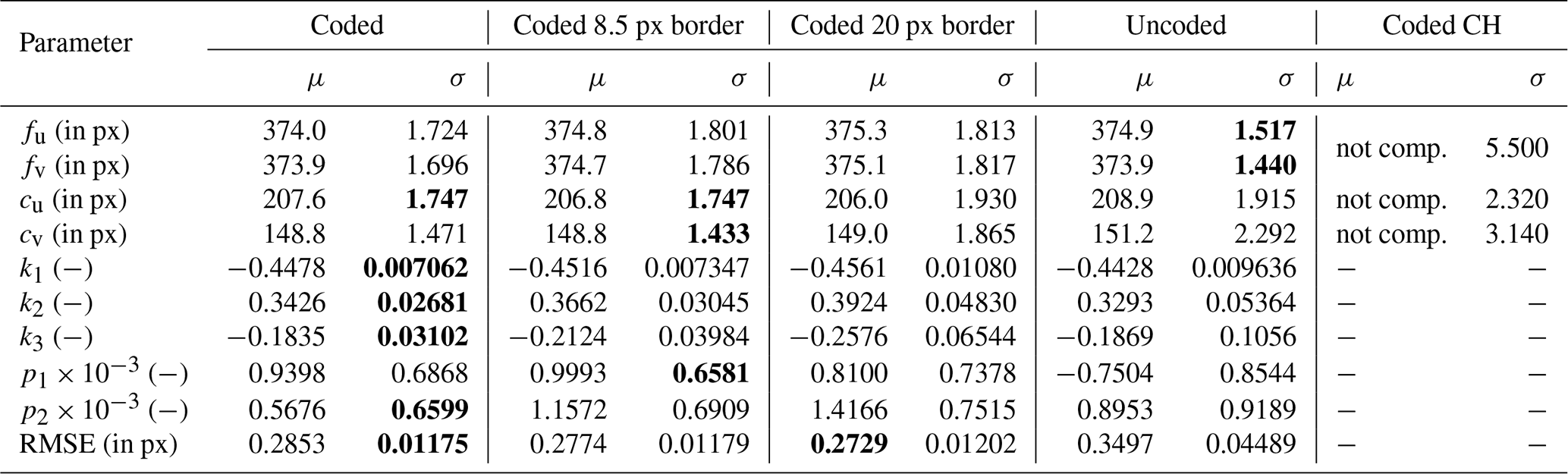
To perform a comparison with the calibration results denoted sep₂₀ in Choinowski et al. (2019), a multicalibration was performed using identical parameters (N=20, M=1000, no percentile filtering). The results are shown in Table 2. Note that the mean values μ are not comparable due to manufacturing tolerances and potentially different focus settings. Hence, only the given standard deviations σ can be compared. In addition, no information on the uncertainty in the distortion parameters is provided in Choinowski et al. (2019). The parameter precision was higher for both of the targets used in this paper. The results were validated by multicalibrations with N=10 and 30, both of which gave the same results as the previous multicalibration.

Besides the three columns allowing a comparison of the three target types, Table 2 has two additional columns, Coded 8.5 px border and Coded 20 px border. The images of the ArUco target were also used in these calibrations, but all features with a distance to the border d_b of <8.5 px or <20 px, respectively, were excluded from the calibration (see Fig. 9). These two values were chosen because 8.5 px corresponds to the theoretical limit from Sect. 4.2 and, when viewing the data from the uncoded checkerboard target, the border distance seen in the heat maps is approx. 20 px (compare Fig. 9c and d). The use of the two additional data sets allows the edge feature detection effect to be separated from other possible dissimilarities between the different targets or the respective data sets. Although the RMSE is slightly reduced, the uncertainty in the parameters increases significantly (by a factor of ≈8 for k₃).

Figure 9 Heat maps of the feature positions for the evaluated variants in Table 2 with N=50.

A comparison of the radial distortion parameters of the data set presented in Table 2 is shown as a boxplot in Fig. 10. Here, in addition to the expected smaller span, it can also be seen that the distribution is more symmetric for the ArUco target. When the p-value from a Shapiro–Wilk test (Shapiro and Wilk, 1965) is higher than 0.05, the test indicates that the set of values tested are normally distributed. This test was performed on 100 randomly selected values from Fig. 10. All ArUco radial distortion coefficients were normally distributed for the coded target ($p_{\mathrm{k}\mathrm{1},\mathrm{ArUco}}=\mathrm{0.853}$, $p_{\mathrm{k}\mathrm{2},\mathrm{ArUco}}=\mathrm{0.336}$ and $p_{\mathrm{k}\mathrm{3},\mathrm{ArUco}}=\mathrm{0.273}$), while k₂ and k₃ were not normally distributed ($W_{\mathrm{k}\mathrm{1},\mathrm{Uncoded}}=\mathrm{0.401}$, $W_{\mathrm{k}\mathrm{2},\mathrm{Uncoded}}=\mathrm{0.004}$ and $W_{\mathrm{k}\mathrm{3},\mathrm{Uncoded}}=\mathrm{8.18}\times {\mathrm{10}}^{-\mathrm{6}}$).

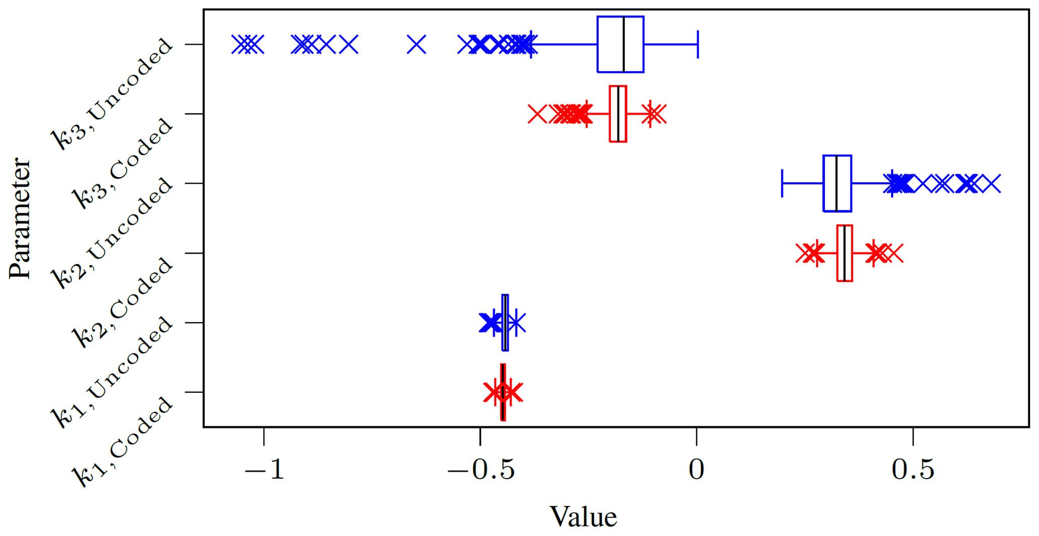
Figure 10 Boxplot comparing the radial distortion parameters k₁, k₂ and k₃ obtained with the coded and uncoded targets.

4.4 Target detection time

Another advantage of using coded targets is that the detection of these marker libraries is optimized for performance. This is especially helpful when the target needs to be detected in real time to check if an image can be used for calibration (and thus the image is included in the data set). This is not an explicit advantage of the presented algorithm, but it is a fundamental advantage when using coded targets.

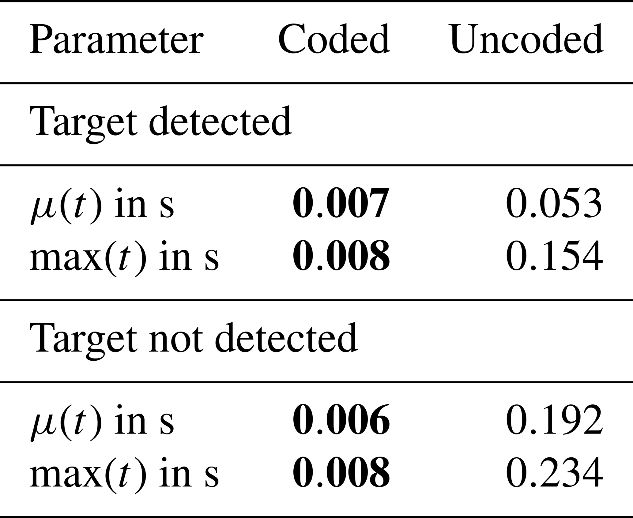
To examine this, the image series was extended by including the images in which the target was not detectable. The specific values depend on the computer used (CPU: Intel i7-10510U, 1.8 GHz), but their ratios demonstrate the differences. Table 3 shows the maximum and average durations of target detection using the OpenCV methods detectMarkers for ArUco and findChessboardCorners for the uncoded target, respectively. There is an extra setting for quickly finding targets in images with findChessboardCorners, but no target was detected in any image when this flag was used. This was probably due to the significantly lower signal-to-noise ratio compared to VIS images. It is noticeable in Table 3 that there are only small differences between detection and nondetection for ArUco markers (−14 % on average), but the image processing time increases significantly for the checkerboard algorithm in the case of nondetection (+262 % on average). Thus, in the case of nondetection, processing took a factor of 32 longer for the uncoded target. Given that the maximum frame rate for the Optris PI 450 is 80 Hz, image data for the uncoded target could not be processed on the computer in real time.

The duration of the actual calibration, which is not usually performed in real time during the measurements, is approximately the duration of the uncoded target calibration multiplied by the number of iteration steps (see Sect. 4.1) compared to the uncoded target.

Table 3 Comparison of the detection times required when using the ArUco marker and the chessboard with OpenCV 4.4.0 for Python. In each case, 40 images were evaluated. The shorter of the two calculation durations (for the coded and uncoded targets) in each case is shown in bold.

5 Discussion

It should first be noted that both targets used in this work had lower standard deviations for f_u, f_v and c_v compared to those reported in Choinowski et al. (2019), and the coded target also had a lower standard deviation for c_v. Thus, in this comparison, the advantage exhibited by the targets used in this work is not solely due to the use of a coded target and iterative evaluation. The active heating of the target as well as the use of the CLAHE algorithm yielded an increased contrast-to-noise ratio, which in turn led to better feature localization (compare to Schramm et al., 2021). Unfortunately, the sizes of the features in the coded circle targets used in the related works (Lagüela et al., 2011; Luhmann et al., 2013; Schmidt and Frommel, 2015) were not described in the images in those works, so a quantitative comparison of border detectability was not possible. To achieve a minimal image border distance d_b of 1.6 px (as shown in Sect. 4.2) with a circle feature target, the circle radius must be the same size. In the calibration images shown in those works, the circles are resolved more finely. Especially in the results presented in Schmidt and Frommel (2015) (Fig. 8, left), it can be seen that features at the border are not detected.

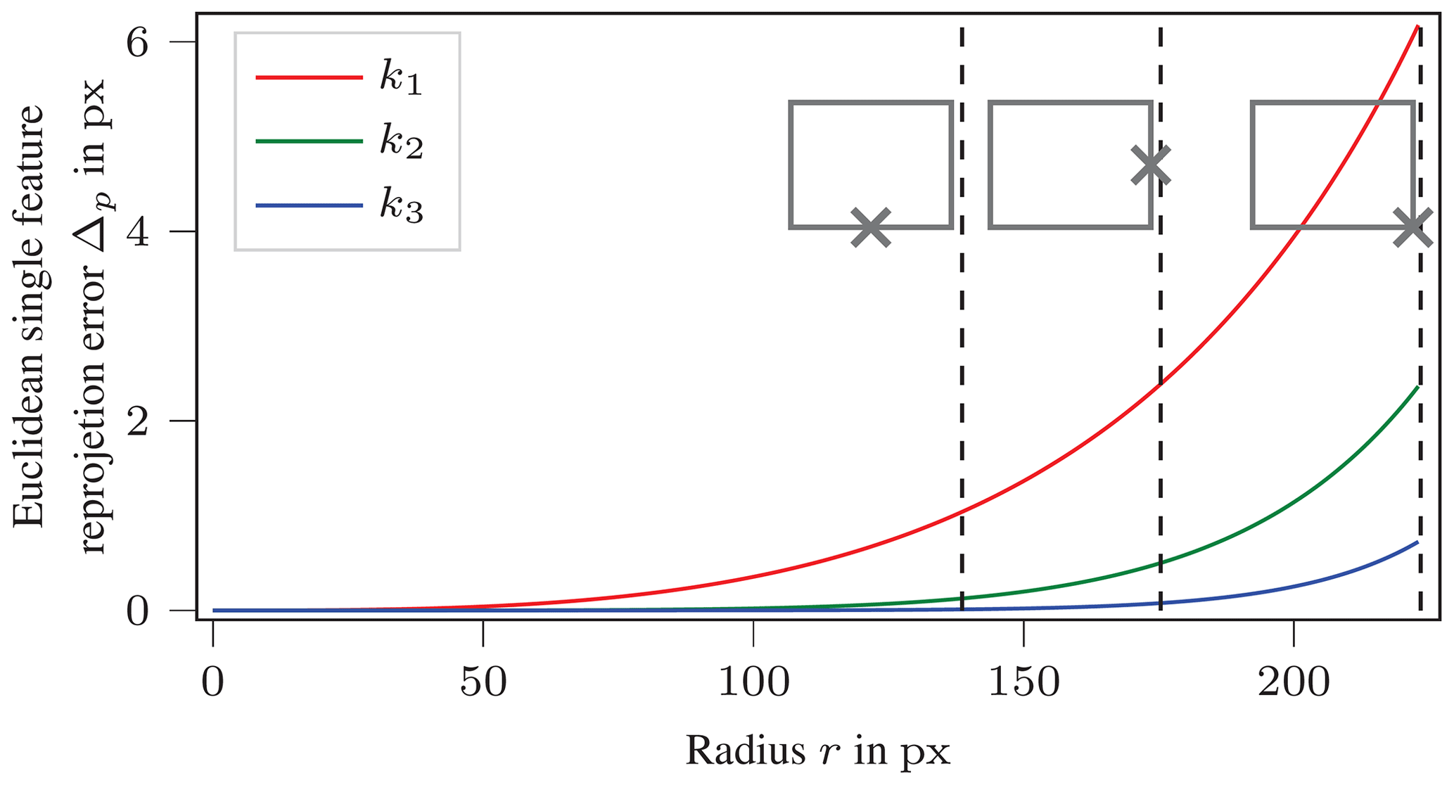
Figure 11 Sensitivity analysis of radial distortion parameters as a function of radius r from the image center. The dashed lines illustrate the r values at the image edges and corners.

The relative decrease in parameter uncertainty obtained with the coded target as compared to the uncoded target was strongest for the radial distortion parameters. At the same time, it was shown that feature positions closer to the image edge can be localized. According to the Brown model, the displacement of a point increases at the edge of the image (differentiate Eq. 2 with respect to k₁, k₂ and k₃, respectively). Figure 11 shows a sensitivity analysis based on the parameters shown in Table 2. A point at radius r (see Eq. 4) from the center of the image (c_u, c_v) is transformed inversely to a 3D point (independent of the distance to the camera coordinate system Z_c) with these parameters. This world point is then mapped back with a single investigated parameter offset by 10 % of its value. The Euclidean distance between the original and the reprojected point indicates the effect of the parameter change. It is clear that as the power of the parameter increases, the influence on the calibration occurs closer to the edge. This demonstrates the relevance of detecting features at image edges to the uncertainty in the calibration parameters. At the same time, it means that the correct parameterization of k₂ and k₃ becomes more important when information from the image edges needs to be used.

At the same time, the features at the image edges have only a small influence on the principal point position c_u, c_v and the tangential distortion parameters p₁ and p₂. The data set obtained without the 8.5 px border features (see Table 2) presents higher ($\mathit{\sigma }\left(p_{\mathrm{2}}\right)=+\mathrm{4.7}\mathrm{\%}$), equal (σ(c_u)) and even slightly lower ($\mathit{\sigma }\left(c_{\mathrm{v}}\right)=-\mathrm{2.7}\mathrm{\%}$ and $\mathit{\sigma }\left(p_{\mathrm{1}}\right)=-\mathrm{4.3}\mathrm{\%}$) standard deviations for these parameters. Even though the distortion model is the standard model for the parameterization of IR and VIS cameras, it does not seem to perfectly describe the distortion that occurs due to the slightly increased RMSE when all points at the border are considered (+4.5 % compared to the 20 px border data set; see Table 2).

The normally distributed parameter estimates obtained with the coded target allow the derivation of direct statements about the uncertainty in the calibration from the empirical standard deviations σ. This can be advantageous if the geometric properties of the calibrated camera are expected to lie within a certain confidence interval.

Furthermore, Sect. 4.4 indicates that the use of rapidly detectable features (independent of the calibration algorithm used) can have advantages for real-time target detection.

Due to the lack of a checkerboard corner detector (aside from during the refinement step), the target may not be occluded during calibration. While it may be partially outside the FOV, the features located in the image FOV must be visible. If, for example, a feature is occluded by the operator's hand, a checkerboard corner is also searched for in this area, and the point with the highest local derivative is returned. Although the effect of a few occluded corners on the overall result is small, these images should be excluded from the data set beforehand. In the case of an uncoded target, an occluded corner will cause the entire target to be undetected and thus automatically excluded. The algorithm presented in Choinowski et al. (2019) avoids the use of such hidden features.

6 Conclusions

Within the scope of this work, a coded target for the geometric calibration of an LWIR camera was developed and evaluated using an iterative feature detection algorithm. Compared to the state of the art, the combination of this target and the algorithm allowed improved feature detection at image borders. This improves the estimation of radial distortion parameters, as indicated by the distortion parameter uncertainty and a sensitivity analysis.

Future work could address the automated preprocessing of the calibration images. Both the ArUco detection of the coded target algorithm and the checkerboard detection of the uncoded target depend on the adaptive contrast enhancement parameters. Currently, the algorithm does not have the ability to identify whether a feature of the target is occluded by another object. A filtering step such as that applied in Wohlfeil et al. (2019) would be useful, but consideration must be given to the issue of whether the feature neighborhood cannot be evaluated entirely at image borders. In addition, extending the calibration from well-known global camera models to local models, as in Schops et al. (2020), could also lead to good results for infrared cameras.