An in-hive soft sensor based on phase space features for Varroa infestation level estimation and treatment need detection

Bees are recognized as an indispensable link in the human food chain and general ecological system. Numerous threats, from pesticides to parasites, endanger bees, enlarge the burden on hive keepers, and frequently lead to hive collapse. The Varroa destructor mite is a key threat to bee keeping, and the monitoring of hive infestation levels is of major concern for effective treatment. Continuous and unobtrusive monitoring of hive infestation levels along with other vital bee hive parameters is coveted, although there is currently no explicit sensor for this task. This problem is strikingly similar to issues such as condition monitoring or Industry 4.0 tasks, and sensors and machine learning bear the promise of viable solutions (e.g., creating a soft sensor for the task). In the context of our IndusBee4.0 project, following a bottom-up approach, a modular in-hive gas sensing system, denoted as BeE-Nose, based on common metal-oxide gas sensors (in particular, the Sensirion SGP30 and the Bosch Sensortec BME680) was deployed for a substantial part of the 2020 bee season in a single colony for a single measurement campaign. The ground truth of the Varroa population size was determined by repeated conventional method application. This paper is focused on application-specific invariant feature computation for daily hive activity characterization. The results of both gas sensors for Varroa infestation level estimation (VILE) and automated treatment need detection (ATND), as a thresholded or two-class interpretation of VILE, in the order of up to 95 % are presented. Future work strives to employ a richer sensor palette and evaluation approaches for several hives over a bee season.

1 Introduction

Major issues from environmental pollution to invasive species are threatening our ecological system and the human food supply. Insects – honey bees in particular – play a decisive role (e.g., for pollination) in maintaining this system. The Varroa mite is a parasite that poses a major threat to bee keeping and is the cause of many bee colony losses. The monitoring of the Varroa infestation level is one important task of conventionally operating bee keepers. Although there is a community practicing treatment-free bee keeping (Hudson and Hudson, 2020) or chemical-free alternatives like thermal treatment (Wimmer, 2020), the majority of bee keepers follows standard treatment practice (e.g., employing formic acid) and needs to know the right time to start treatment based on the hive infestation level. In general, access to information on the current hive infestation level without having to disturb the bees would be of high value, independent of the treatment method. Sensors and automation (Werthschützky, 2018), like in home automation (Eric Mounier, 2017), automated agriculture (Rembert, 2020), condition monitoring (Lee et al., 2011; IEEE, 2015; Zhang et al., 2017; Weckbrodt, 2019), and Industry 4.0 (Kagermann et al., 2011; Kohlert and König, 2016), can both alleviate hive keeping and make it much more effective. Thus, over the last 10–15 years, numerous approaches to digital bee keeping have been observed (e.g., Ohashi et al., 2009; Cecchi et al., 2020; Gil-Lebrero et al., 2017; Kulyukin et al., 2018; Nolasco et al., 2018; Wallich, 2011; Suta, 2014; Bromenschenk et al., 2007; König, 2019). In our IndusBee4.0 project, small, effective, and affordable cognitive integrated sensor systems (i.e., acting as a soft sensor) for continuous in-hive monitoring and state estimation (e.g., monitoring and reporting the Varroa infestation level) are pursued. In particular, affordable integrated gas sensors, namely SGP30 (SENSIRION, 2022; Rüffer et al., 2018) or BME680 (Bosch, 2020) sensors, and suitable domain-specific features are of interest here. Although individual sensor readings can already provide meaningful information on the Varroa infestation level estimation (VILE) and the automated treatment need detection (ATND), the focus of this paper is on the investigation of increasingly invariant feature computation based on a phase space abstraction to hive activity over day cycles. The approach, the most meaningful features, and possible recognition rates will be presented and compared to the individual sensor readings.

2 Ground truth determination by conventional Varroa monitoring

There are several standard methods available for conventional VILE. A common feature of these methods is that they all imply substantial effort for the bee keeper and deliver results only at larger time steps. The analysis of hive debris, including mites dropping from the hive bottom that are collected on a slider or Varroa board, is the most common technique (Bayerische Landesanstalt für Weinbau und Gartenbau, 2021). Usually, a probing time (t_p) of 3 days is expended until a manual (or more recently (semi) automated vision-based) analysis of the debris for the number of dropped Varroa (N_d) can be conducted. The ground truth of the hive infestation level (GT) or current Varroa population size can be estimated from this count (Bayerische Landesanstalt für Weinbau und Gartenbau, 2021; König, 2019) by employing a scaling factor, e.g., F_s=150:

$$\begin{array}{}\text{(1)}& \mathrm{GT}=F_{\mathrm{s}}\times {\displaystyle \frac{N_{\mathrm{d}}}{t_{\mathrm{p}}}}.\end{array}$$

Another common approach, also denoted as the flotation method, extracts a bee sample from the hive and submerges the sample in water (drowning the bees) to separate the bees and Varroa mites. The powdered sugar and CO₂-based sedation methods are two alternative, more bee-friendly variants. Again, the hive infestation level can be estimated from a count, but the sample adequateness will probably depend on the location of extraction in the hive. More recent principle approaches try to scrutinize in- and outgoing bees at the flight hole for Varroa mites clinging to them (e.g., Chazette et al., 2016; König, 2019); however, all methods based on the count of mites clinging to bees are not able to give an immediate reckoning of the mite population in the brood.

Thus, in this work, standard counting on a Varroa board was applied to obtain the required GT for VILE and ATND, but a higher-than-standard inspection frequency was used (approximately twice on average throughout the bee season) in order to obtain an improved temporal analysis of the hive infestation state.

3 Measurement approach and system

With regard to the objective of finding a solution that is unobtrusive to bees, a compact realization is aspired to, even for the first prototype, for the hive monitoring system: it should not consume significant volume in the supporting comb nor significantly limit hive traffic routes and air ventilation. Limited power consumption and cost were further sensor selection criteria. The block diagram of the IndusBee4.0 apiary hive monitoring system is given in Fig. 1, which enumerates the current sensor palette: the standard DHT22 T/RH (temperature and relative humidity) sensors (Adafruit, 2021); the HX711 (AVIA Semiconductor, 2020) weight sensor module with four standard weight cells for hive, honey storage, or feeder module scale implementation; a Knowles SPH0645 MEMS (micro-electromechanical system) microphone (Knowles, 2021) for vibration and sound recording; and the SGP30 (SENSIRION, 2022) and BME680 (Bosch, 2020) gas sensors. One SmartComb unit with the number and placement of the named sensor types is shown in Fig. 2. This instrumented comb is placed in the center (slot 5 of 10) in the middle or center super of the regarded three-super hive. This placement situated the sensors close to the center of breeding activity and associated Varroa occurrence. The measurement system was programmed in Python, employing existing libraries for the sensors where possible: the Adafruit library for the DHT22 (Adafruit, 2021); the HX711 library (Zak, 2020) in its Python 2 version; the Pimoroni libraries for the SGP30 (Pimoroni, 2020b), employing the DHT22 RH reading and the required absolute humidity (AH) computation algorithm from Mander (2021), and the BME680 (Pimoroni, 2020a); and the scikit-learn package (Pedregosa et al., 2011) in Python for the machine learning part. Recently, much more efficiently integrated universal sensor platforms (USePs) have emerged, such as the USeP research platform and the follow-up Sensry platform (Sensry, 2021), which have quite similar sensor portfolios. Basic investigations in the past have revealed that both the sound patterns emitted by bees and the air composition inside the hive host information that correlates with the Varroa infestation level, as determined by the conventional methods outlined in the previous section. Hive sound patterns also allow one to detect information on factors such as a “missing queen” or the development of “swarming mood”. Thus, in our work and in many previous studies, microphones and signal processing analysis have been applied (Kulyukin et al., 2018; Nolasco et al., 2018; Bromenschenk et al., 2007; König, 2019). MEMS microphones deliver the acoustic information on the hive state in our Pi-Zero-W-based SmartComb in-hive measurement system, including continuous cues for VILE in a multi-sensor or soft sensor approach. Recent intriguing work, based on a set of Figaro gas sensors and an external measurement system, confirmed the existence and usefulness of a correlation between hive air analysis results and the Varroa infestation level (Szczurek et al., 2019, 2020a; Ba̧k et al., 2020). With the advent of highly integrated gas sensing systems, such as the Sensirion SGP30 multi-pixel gas sensor system¹ (SENSIRION, 2022) or the BOSCH Sensortec BME680 (Bosch, 2020), the possibility for VILE using an in-hive low-cost gas sensing system and (in)direct indicators from hive air analysis over the bee season was added to our IndusBee4.0 system. Numerous projects exploiting these and other sensor chips have recently been carried out; these studies have predominantly focused on air quality issues (e.g., Arroyo et al., 2020), but breath analysis (Jaeschke et al., 2019) has also been carried out and inspired the use case in this work. The BME680 allows for the control of a sensor hot plate or the heating of the single gas sensor pixel, i.e., it can be modulated for temperature cycles (Lee and Reedy, 1999; Jaeschke et al., 2019) in measurement. One significant advantage of a hive-integrated solution is measurement in the stable “bee climate”, which avoids numerous issues such as those related to the dew point that have been reported for external measurement setups (Szczurek et al., 2020a; Ba̧k et al., 2020).

Figure 1 Overview of the IndusBee4.0 apiary monitoring system with SmartComb units including BeE-Nose for VILE (adapted from König, 2021a).

4 Feature computation

Although instantaneous sensor readings can already be useful, as will be outlined in the following section, several issues with regard to sensor nonuniformity, drift, dynamics, or other temporal dependencies can advocate for the calculation of meaningful invariant features, as common in most pattern recognition applications. In gas sensing, normalization of sensor readings to a baseline value and/or compression by logarithm computation are the most common steps. Other techniques are the calculation of statistical or frequency domain features, such as the mean value, standard deviation, or spectral features. In particular, the dynamics of gas sensors under temperature modulation inspired the use of a technique from general systems theory related to the concept of phase space (PS) and features calculated from the resulting trajectories. There is an interesting relationship between established blob analysis and blob description by features in vision problems (e.g., lucidly described in Mallick, 2021) and phase space trajectory analysis and description by related features. The concept of phase space trajectory computation and description by meaningful compact features can be found in studies such as Martinelli et al. (2003) and Penza et al. (2009), where it serves to generate features from sensor dynamics observed for appropriately thermically modulated gas sensors.

This proven approach, employing, for instance, so-called dynamic moments (DM) (Penza et al., 2009) or energy vectors (EV) is very attractive, and it inspired the investigation of the abstraction of the concept to the observable dynamics of a bee hive (e.g., Khoury et al., 2013; Russell et al., 2013), associating the dynamics of a daily activity cycle with the temperature modulation cycle of a sensor. With this aim, the data reported in the next section will be grouped into 24 h cycles, from midnight to midnight, and an abstraction of the phase space concept and related features will be computed. In the simplest case, a phase space can be generated by the temporal measurement series and its derivative (Penza et al., 2009). A plot of these two quantities will return trajectories reflecting hive activity, which is assumed here to be affected or modulated by the Varroa infestation level, and descriptive features can be calculated for ensuing classification. This will reduce the weaknesses of instantaneous sensor readings, and, in contrast to the “real-time” character of bee swarm indication, the VILE or ATND can be reported on a less challenging timescale. The heuristic finding of the following descriptive features for the resulting trajectories in the phase space abstraction was inspired by standard blob analysis features (e.g., centroid and area, circumference) and Penza et al. (2009), leading to the ensuing list:

The first feature, ${\stackrel{\mathrm{‾}}{d}}_{i\mathrm{Norm}}$, is the daily mean of the sensor reading $\stackrel{\mathrm{‾}}{d_i}$ normalized by the mean number of days (NoD) in the campaign (which is calculated as $C_{\mathrm{m}}=\frac{\mathrm{1}}{\mathrm{NoD}}{\sum }_i^{\mathrm{NoD}}\stackrel{\mathrm{‾}}{d_i}$):

$$\begin{array}{}\text{(2)}& {\stackrel{\mathrm{‾}}{d}}_{i\mathrm{Norm}}={\displaystyle \frac{{\stackrel{\mathrm{‾}}{d}}_i}{C_{\mathrm{m}}}}.\end{array}$$

The second feature, ${\stackrel{\mathrm{‾}}{\mathrm{dd}}}_{i\mathrm{Norm}}$, is the daily mean of the sensor reading derivative ${\stackrel{\mathrm{‾}}{\mathrm{dd}}}_i$ normalized by the campaign maximum value of the derivatives, Cd${}_{\mathrm{m}}={max}_{i=\mathrm{1}}^{\mathrm{NoD}\cdot {\mathrm{ddc}}_i}{\mathrm{dd}}_i$, where ddc_i is the number of derivative values per day:

$$\begin{array}{}\text{(3)}& {\stackrel{\mathrm{‾}}{\mathrm{dd}}}_{i\mathrm{Norm}}={\displaystyle \frac{{\stackrel{\mathrm{‾}}{\mathrm{dd}}}_i}{{\mathrm{Cd}}_{\mathrm{m}}}}.\end{array}$$

The third feature, tlength, is the length of the daily trajectory normalized by the number of measurements of the regarded day, dc_i, in phase space:

$$\begin{array}{}\text{(4)}& \mathrm{tlength}={\displaystyle \frac{\mathrm{1}}{{\mathrm{dc}}_i}}\sum _{i=\mathrm{2}}^{{\mathrm{dc}}_i}\left(\right|d_i-d_{i-\mathrm{1}}|+|{\mathrm{dd}}_i-{\mathrm{dd}}_{i-\mathrm{1}}\left|\right).\end{array}$$

The fourth feature, tangle, is the accumulated angle of the daily trajectory:

$$\begin{array}{}\text{(5)}& \mathrm{tangle}=\sum _{i=\mathrm{2}}^{{\mathrm{dc}}_i}\left(\arctan {\displaystyle \frac{(d_i-d_{i-\mathrm{1}})}{({\mathrm{dd}}_i-{\mathrm{dd}}_{i-\mathrm{1}}}}\right).\end{array}$$

The fifth feature, $d_{i\mathrm{Norm}}^{\mathrm{maxr}}$, is the ratio of the maximum sensor reading and the maximum derivative ${\stackrel{\mathrm{‾}}{\mathrm{dd}}}_i$, each normalized as given in Eqs. (2) and (3), respectively:

$$\begin{array}{}\text{(6)}& d_{i\mathrm{Norm}}^{\mathrm{maxr}}={\displaystyle \frac{d_i^{\max }/C_{\mathrm{m}}}{{\mathrm{dd}}_i^{\max }/{\mathrm{Cd}}_{\mathrm{m}}}}.\end{array}$$

The sixth feature, $d_{i\mathrm{Norm}}^{\mathrm{minr}}$, is the ratio of the minimum sensor reading and the minimum derivative ${\stackrel{\mathrm{‾}}{\mathrm{dd}}}_i$, each normalized as given in Eqs. (2) and (3), respectively:

$$\begin{array}{}\text{(7)}& d_{i\mathrm{Norm}}^{\mathrm{minr}}={\displaystyle \frac{d_i^{\min }/C_{\mathrm{m}}}{{\mathrm{dd}}_i^{\max }/{\mathrm{Cd}}_{\mathrm{m}}}}.\end{array}$$

The respective seventh and eighth features, $d_i^{\mathrm{spanC}}$ and ${\mathrm{dd}}_i^{\mathrm{spanC}}$, give the span center of the sensor readings and sensor readings' derivative displaced by the respective minimum value:

$$\begin{array}{}\text{(8)}& {\displaystyle }{d}_i^{\mathrm{spanC}}={\displaystyle \frac{\frac{d_i^{\max }-d_i^{\min }}{\mathrm{2}}+d_i^{\min }}{C_{\mathrm{m}}}},\text{(9)}& {\displaystyle }{\mathrm{dd}}_i^{\mathrm{spanC}}={\displaystyle \frac{\frac{{\mathrm{dd}}_i^{\max }-{\mathrm{dd}}_i^{\min }}{\mathrm{2}}+{\mathrm{dd}}_i^{\min }}{{\mathrm{Cd}}_{\mathrm{m}}}}.\end{array}$$

Features 9 to 13 correspond to the dynamic moment calculations given in Penza et al. (2009), denoted as DM2, DM3_X, DM3_Y, DM3_PB, and DM3_SB, respectively:

$$\begin{array}{}\text{(10)}& {\displaystyle }\mathrm{DM}\mathrm{2}={\displaystyle \frac{\mathrm{1}}{{\mathrm{dc}}_i}}\sum _{i=\mathrm{1}}^{{\mathrm{dc}}_i}(d_i\times {\mathrm{dd}}_i),\text{(11)}& {\displaystyle }\mathrm{DM}{\mathrm{3}}_{\mathrm{X}}={\displaystyle \frac{\mathrm{1}}{\mathrm{2}\times {\mathrm{dc}}_i}}\sum _{i=\mathrm{1}}^{{\mathrm{dc}}_i}({d_i}^{\mathrm{3}}-\mathrm{3}\times d_i\times {{\mathrm{dd}}_i}^{\mathrm{2}}),\text{(12)}& {\displaystyle }\mathrm{DM}{\mathrm{3}}_{\mathrm{Y}}={\displaystyle \frac{\mathrm{1}}{\mathrm{2}\times {\mathrm{dc}}_i}}\sum _{i=\mathrm{1}}^{{\mathrm{dc}}_i}(d_i^{\mathrm{3}}-\mathrm{3}\times {d_i}^{\mathrm{2}}\times {\mathrm{dd}}_i),\text{(13)}& {\displaystyle }\mathrm{DM}{\mathrm{3}}_{\mathrm{PB}}={\displaystyle \frac{\sqrt{\mathrm{2}}}{{\mathrm{dc}}_i}}\sum _{i=\mathrm{1}}^{{\mathrm{dc}}_i}({d_i}^{\mathrm{2}}\times {\mathrm{dd}}_i-d_i\times {{\mathrm{dd}}_i}^{\mathrm{2}}),\text{(14)}& {\displaystyle }\mathrm{DM}{\mathrm{3}}_{\mathrm{SB}}={\displaystyle \frac{\sqrt{\mathrm{2}}}{{\mathrm{dc}}_i}}\sum _{i=\mathrm{1}}^{{\mathrm{dc}}_i}(\mathrm{2}\times d_i^{\mathrm{3}}+\mathrm{3}\times ({d_i}^{\mathrm{2}}\times {\mathrm{dd}}_i-d_i\times {{\mathrm{dd}}_i}^{\mathrm{2}}\left)\right).\end{array}$$

Feature 14, NoSC, adds information on the number of direction changes derived from the angle sign changes according to feature 4 (Eq. 5):

$$\begin{array}{}\text{(15)}& {\displaystyle }{\mathit{\alpha }}_i=\arctan \left({\displaystyle \frac{(d_i-d_{i-\mathrm{1}})}{({\mathrm{dd}}_i-{\mathrm{dd}}_{i-\mathrm{1}})}}\right),\text{(16)}& {\displaystyle }\mathrm{NoSC}=\sum _{i=\mathrm{2}}^{{\mathrm{dc}}_i}\left(\mathrm{Sign}\right({\mathit{\alpha }}_i)\ne \mathrm{Sign}({\mathit{\alpha }}_{i-\mathrm{1}}\left)\right).\end{array}$$

Features 15 and 16 add information on the daily span of original and derived signal normalized by the respective normalization value:

$$\begin{array}{}\text{(17)}& {\displaystyle }{d}_i^{\mathrm{spanC}}={\displaystyle \frac{{d_i}^{\max }-{d_i}^{\min }}{C_{\mathrm{m}}}},\text{(18)}& {\displaystyle }{\mathrm{dd}}_i^{\mathrm{spanC}}={\displaystyle \frac{{{\mathrm{dd}}_i}^{\max }-{{\mathrm{dd}}_i}^{\min }}{{\mathrm{Cd}}_{\mathrm{m}}}}.\end{array}$$

This set of features with the described normalization will be calculated in the experiments outlined in the next section, based on the obtained and smoothed gas sensor readings from the SGP30 eCO₂ and total volatile organic compound (TVOC) outputs and the BME680, and will be selectively used in the ensuing classifications with either four or two classes. Details of the methods and parameter settings are given in the next section.

5 Experiments and results

One SmartComb module, given in Fig. 2, was deployed in a mature hive that had released a swarm, and sensor data on temperature, relative humidity, weight, and hive sound as well as gas sensor data from hive air were collected from 8 July to 11 September until formic acid treatment. A baseline in this work was to look for indirect indications of the hive state from the sensor readings (König, 2021a), i.e., deviations from a normal state correlating with mite infestation. The direct indication or detection of certain gas components and absolute quantities (e.g., originating from the mites' metabolism) is a more ambitious and more costly next step that will require increased effort from the sensor portfolio to the data evaluation. The acquired and archived measurement data were processed based on standard Python. In the first step, a moderate smoothing of the data, sampled at approximately six samples per minute, was conducted using a digital low-pass filter from the SciPy signal package (The SciPy community, 2021) with the corner parameter set to 0.1. The smoothing settings have an immediate influence on the achievable classification rates of the following experiments.

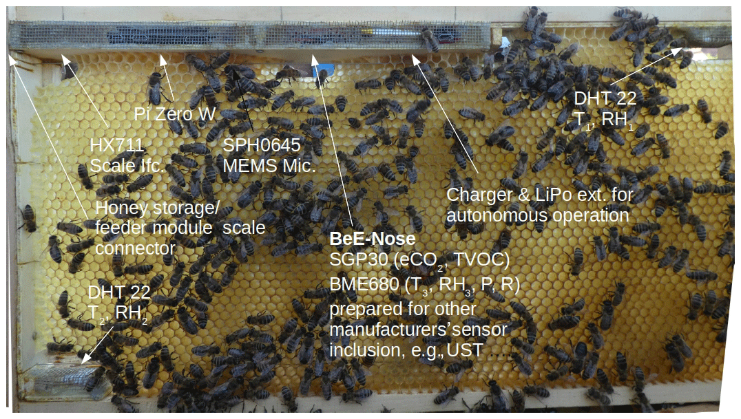
Figure 2 The SmartComb unit related to the reported measurements, including BeE-Nose for VILE.

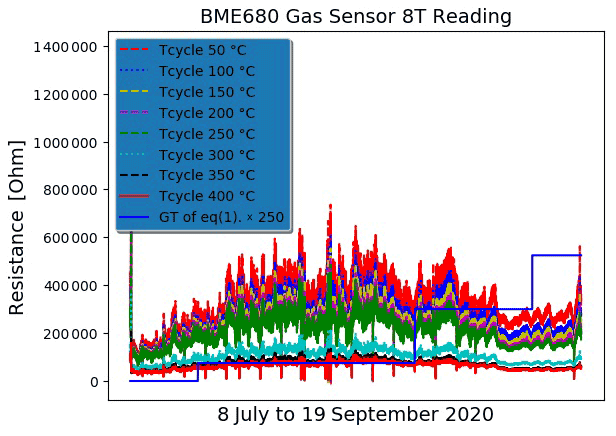
Figure 3 BME680 resistance data for the period from 8 July to 11/19 September for temperature steps from 50 to 400 ^∘C as well as the scaled-up Varroa count GT.

Figure 3 shows a subset of gas sensing measurements from the BME680 for eight temperature steps as well as the Varroa counting GT, the latter of which was scaled-up for the sake of visual representation, corresponding to the description in Sect. 2 for this campaign for 56 (58) d from 8 July to 11 (19) September 2020². The SGP30 (SENSIRION, 2022) and the BME680 (Bosch, 2020) gas sensors both served for measurement in this campaign. The SGP30 delivers both eCO₂ and TVOC outputs as well as two additional outputs, denoted as Raw₁ and Raw₂ for hydrogen and ethanol, respectively. Results obtained for the SGP30 standard use in this application have been reported in König (2021b). The BME680 gives a single resistance value, which was acquired here for eight equidistant levels from 50 to 400 ^∘C in a basic staircase-shaped temperature cycle with an approximate 500 ms step time and the sensor reading at the end of the step time. These measurements from both sensors were directly employed in the first step as features for the VILE and ATND based on a hold-out approach: 837 samples per training and test set were extracted from the complete measurement data in steps of 250 with a displacement between the training and testing data of 125.

With regard to VILE, the problem has been simplified into four discrete steps or levels derived from the GT described in Sect. 2: No Varroa, Low Varroa, Mid Varroa, and Treatment !, corresponding to counted daily averages of 0, 2.5, 8.6, and 14 Varroa on the board from 3 days of screening in four inspection runs. With the established treatment threshold value of 10, the last daily average is definitely above the threshold. However, due to the sparseness of GT sampling, there are several days that are actually a better fit with the Treatment ! class than with the Mid Varroa class with which they were affiliated. The acquired data set, which actually ended with the onset of formic acid treatment, was extended by 2 days, 18 and 19 September, after the first week of treatment. These additional samples, extending the campaign to 58 d, can be affiliated with the Treatment ! class. To elucidate if 1 week of formic acid treatment had a perceivable effect, a fifth class, “Post-treatment”, was added for illustration purposes in the following (see Fig. 7).

For ATND, the first three classes are merged into the “SubTh” class, denoting a sensor reading below the treatment threshold. In this case, the 2 extra days after the first week of formic acid treatment are either labeled as Treatment ! or as SubTh. Figure 4 illustrates a scatterplot of the first and seventh BME680 temperature steps, showing a weak to moderate support for the VILE hypothesis. Table 1 shows the classification results, based on the scikit-learn package (Pedregosa et al., 2011) and the included k-nearest neighbor (kNN) classifier, for the BME680 data from the campaign as well as the described VILE and ATND class labels and the hold-out approach (Pedregosa et al., 2011, and Fukunaga, 1990; from p. 219 and p. 310, respectively) for all eight temperature steps. The results coincide with the scatterplot in Fig. 4 and are quite similar to previously obtained results from the SGP30 (König, 2021b).

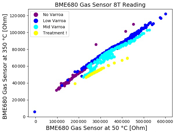
Figure 4 Campaign data for the period from 8 July to 11/19 September for the BME680 sensor at 50 and 350 ^∘C.

Table 1 Classification results for BME680 data using the hold-out approach for the 8 July to 19 September campaign with kNN (k=3).

The approach described so far has been based on the use of instantaneous sensor readings; however, this technique is restricted, as there is an obvious temporal dependence of information on the time of acquisition and/or on the sequence of sensory readings.

Recently, there have been investigations indicating that the time of day matters in this kind of measurement and interpretation (Szczurek et al., 2020b). For this reason, data between 12:00 and 13:00 CET, as a time of commonly high hive activity, have been extracted from the database. Due to the significant reduction in samples in only 1 h of a 24 h period, the hold-out approach was modified to 1814 samples per training and test set, which were extracted from the complete measurement data set in steps of 5 and with a displacement between the training and testing data of just 3. Figure 5 shows the resulting scatterplot of the BME680 sensor at 50 and 350 ^∘C, and Table 2 gives the corresponding classification results again for all eight readings from the eight temperature levels; however, both visual assessment of the plot and repetition of the hold-out classification does not (with regard to the increased similarity of the training and test set) show significant improvement or change compared with the complete data.

Figure 5 The extraction of campaign data for the period from 12:00 to 13:00 CET for the BME680 sensor at 50 and 350 ^∘C.

Table 2 Classification results for BME680 data using the hold-out approach for the 8 July to 19 September campaign for the period between 12:00 and 13:00 CET.

To advance from the evaluation of instantaneous sensor values to an analysis of hive daily activity, as well as to better cope with hive and sensor variations, the available database has been grouped into daily cycles, and (following the concept outlined in Sect. 4) a simple phase space with the original sensor readings on the abscissa and their first temporal derivative on the ordinate has been computed for each day and each sensor output or channel. Each phase space axis has been normalized by the corresponding campaign mean or maximum value, respectively, giving axes values without units. As a first example, Fig. 6 shows the resulting phase space trajectories for the whole campaign for the BME680 sensor at 50 ^∘C, with the class affiliation emphasized by the corresponding color, as employed and indicated in the legends of all scatterplots (e.g., in Fig. 5). Figure 7 shows a scatterplot of phase space features ${\stackrel{\mathrm{‾}}{d}}_{i\mathrm{Norm}}$ and ${\stackrel{\mathrm{‾}}{\mathrm{dd}}}_{i\mathrm{Norm}}$ for the phase space of Fig. 6 and the four classes of VILE as well as the 2 post-treatment days (in green). This plot suggests that the hive state gradually tends to move back to normal after 1 week of treatment.

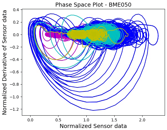
Figure 6 A phase space example of campaign data for the BME680 sensor at 50 ^∘C and the four classes of VILE.

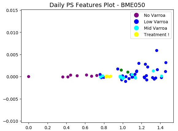
Figure 7 An example of phase space features ${\stackrel{\mathrm{‾}}{d}}_{i\mathrm{Norm}}$ and ${\stackrel{\mathrm{‾}}{\mathrm{dd}}}_{i\mathrm{Norm}}$ for the BME680 sensor at 50 ^∘C and the four classes of VILE as well as the 2 post-treatment days (in green).

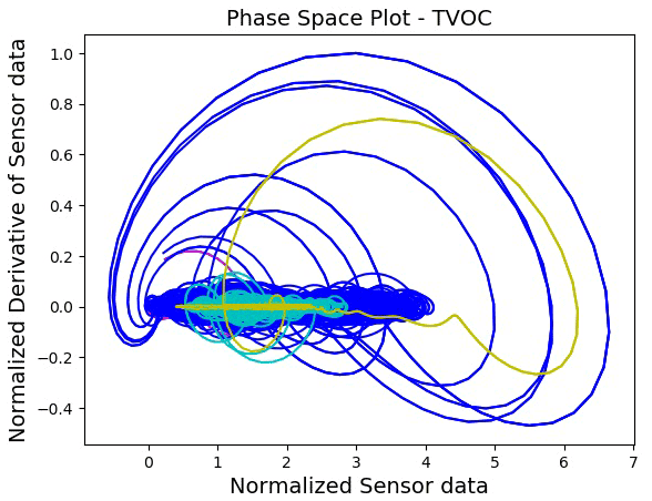
Figure 8 A phase space example of campaign data for the SGP30 sensor, TVOC output, and the four classes of VILE.

Figure 8 shows the corresponding information for the concurrently measuring SGP30 sensor and its TVOC output. The trajectory families associated with the four classes in Figs. 6 and 8 obviously show promising interclass differences for a useful feature computation. Thus, from these daily trajectories in the phase space, features can be computed as outlined in Martinelli et al. (2003) and Penza et al. (2009) and extended upon in Sect. 4. From the 16 available features computed for every sensor output, the most relevant ones have been identified by common feature selection techniques. Summarizing, the daily means ${\stackrel{\mathrm{‾}}{d}}_{i\mathrm{Norm}}$ and ${\stackrel{\mathrm{‾}}{\mathrm{dd}}}_{i\mathrm{Norm}}$, the trajectory length (tlength), the trajectory angle (tangle), and the trajectory number of sign change (NoSC) provide the most promising performance in this particular use case. The promise in the pursued modeling and feature computation is not so much the gain in recognition rate for one particular hive and sensor system; instead, it exists in the improvement of the invariance with regard to factors such as readings from different hives and sensor/measurement systems. This would be required to effectively deploy a functional VILE or ATND unit to all hives of an apiary or to different apiaries.

For this aim, the daily trajectory length (tlength) from Sect. 4, e.g., calculated from SGP30 eCO₂ and TVOC outputs and related phase spaces, was selected. The resulting two-dimensional data already gave both compact and suitable results. Figure 9 shows the scatterplot of the tlength feature for SGP30 eCO₂ and TVOC outputs. Table 3 shows the related classification results for kNN (k=1), a hold-out approach and ATND two-class labeling, where every second day samples were added to the test set and the other half were added to the training set, as well as the result of a leave-one-out (loo) validation run, as the number of days (and, thus, the available number of samples) is sparse compared with the use of instantaneous values.

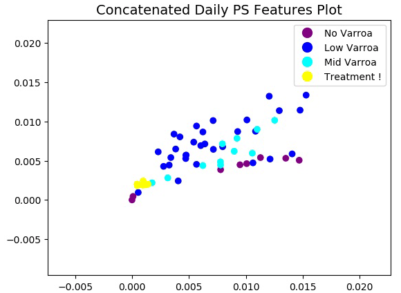
Figure 9 Scatterplot of the tlength feature for the SGP30 eCO₂ and TVOC outputs and the four classes of VILE.

Table 3 Classification results of the tlength feature from the SGP30 eCO₂ and TVOC outputs and the 8 July to 19 September campaign data with kNN (k=1) and the ATND two-class labeling.

To tentatively validate the approach and the underlying feature computation, data from a second campaign acquired from a different hive and different measurement system instance, equipped only with the SGP30 gas sensor, in 34 d of May and June 2020 for SGP30 eCO₂ and TVOC outputs were reactivated. There was no calibration of the two sensor systems with regard to each other. As reported in König (2021a), the investigated hive unfortunately collapsed and perished before the Varroa population crossed the treatment need threshold. Therefore, data are only available for three classes, No Varroa, Low Varroa, and Mid Varroa. The Mid Varroa level is only represented by the last day of this campaign. Thus, for a first invariance investigation of the proposed feature computation, for both data sets from the two campaigns, the No Varroa and Low Varroa classes and the Mid Varroa and Treatment ! classes were merged into two respective classes as a modified ATND. Corresponding to Fig. 9, Fig. 10 shows the training (circles) and test (triangles) data sets from these two different hives. Classifier training and resubstitution then took place with the first campaign, and generalization was done with the second campaign, again using a kNN with k=1. Table 4 shows the results obtained. Moreover, Fig. 11 shows the first and second principle components of all 16 features for SGP30 eCO₂ and TVOC outputs, i.e., 32 features, for both campaigns as well as the two classes of VILE used in the classification given in Table 4. Finally, Fig. 12 shows the first and second linear discriminant analysis (LDA) components for the same data and class affiliation.

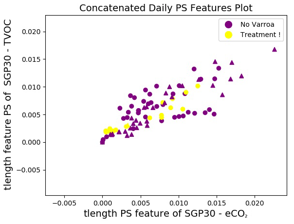
Figure 10 Scatterplot of the tlength feature for the SGP30 eCO₂ and TVOC outputs for cross classification of the July–September (circles) and additional May–June (triangles) campaigns with two classes of VILE.

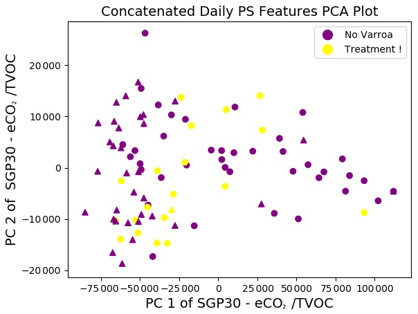
Figure 11 Scatterplot of the first and second principal components of the SGP30 eCO₂ and TVOC outputs for cross classification of the July–September (circles) and additional May–June (triangles) campaigns with two classes of VILE.

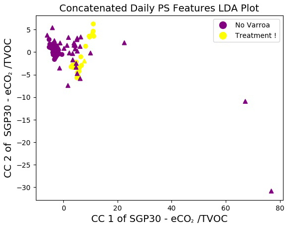
Figure 12 Scatterplot of the first and second LDA components of the SGP30 eCO₂ and TVOC outputs for cross classification of the July–September (circles) and additional May–June (triangles) campaigns with two classes of VILE.

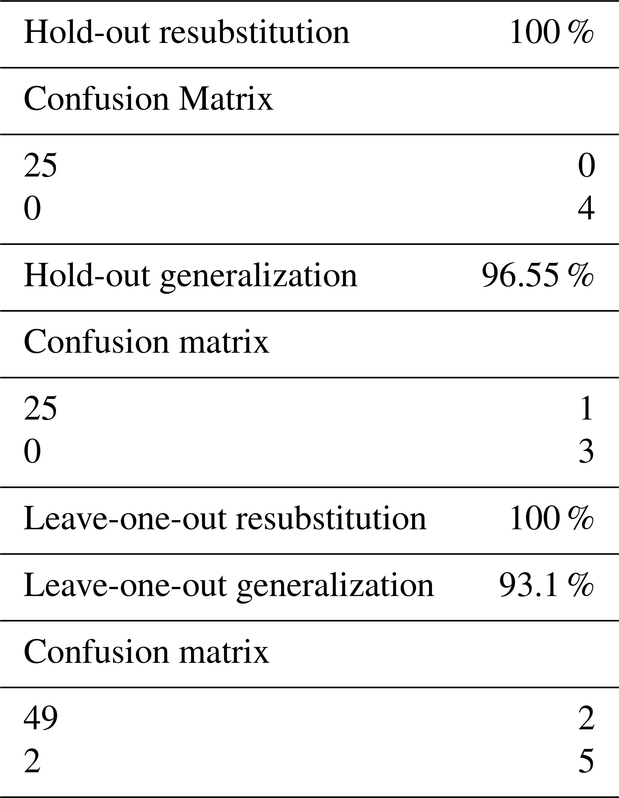
Table 4 Cross classification of the July–September and May–June campaigns with kNN (k=1).

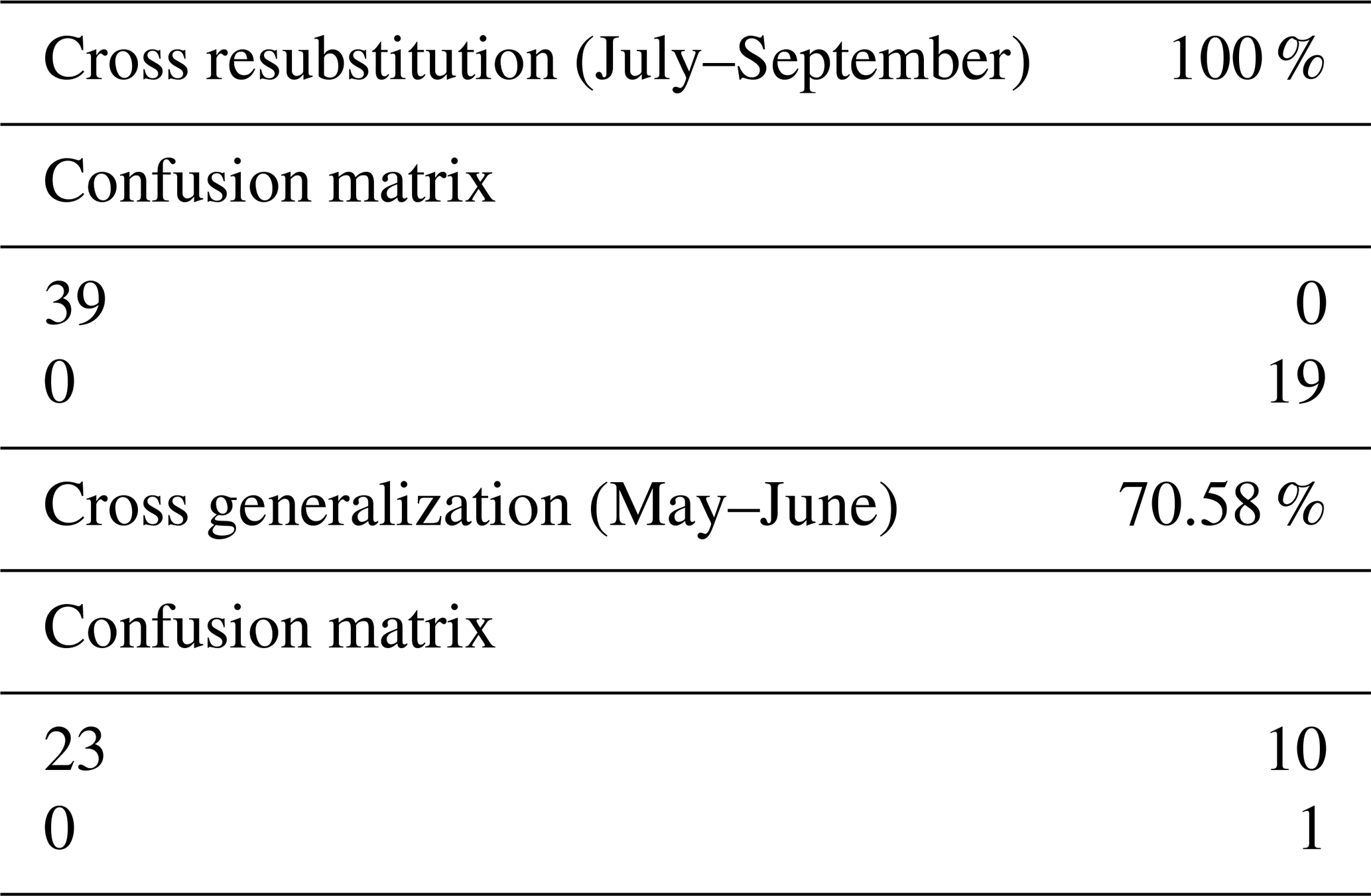
Although there are 10 false positives, the single true positive day was detected. Classification runs with the principal component analysis (PCA) and LDA two-dimensional data gave an identical resubstitution but inferior generalization. This last experiment suggests that the proposed modeling and feature computation provides a baseline for invariant feature computation based on hive activity. Integration of data from several hives and campaigns as well as enlargement of the calibrated sensor spectrum has the potential to further advance the approach. The sparseness of the currently available data has to be overcome by concurrently monitoring a larger number of hives over the entire bee season.

6 Conclusions

Motivated by the importance of honey bees and the increasing challenges imposed on bees and beekeepers, an in-hive close-to-brood nest sensing system was conceived and applied in a single colony for a substantial period of time during the 2020 bee season in a single measurement campaign. One major goal of this work was to obtain an useful estimate of the Varroa infestation level (VILE) and the treatment need level (ATND) from indirect cues obtained from the noninvasive and continuous monitoring of bee hives by simple and cost-effective multi-sensor systems, effectively creating a soft sensor for VILE and ATND. The underlying measurement system and the first results for the SGP30 sensor have already been reported in König (2021a) and König (2021b). In this paper, the focus is on the extension to the BME680 sensor along with temperature modulation (König, 2021c) as well as an approach to invariant feature computation, based on the adoption of the phase space concept related to hive daily activity. From phase space daily trajectories, features from the literature (Martinelli et al., 2003; Penza et al., 2009) and custom heuristic additional features have been computed.

The classification results obtained for both instantaneous sensor readings and the abovementioned phase-space-based features are encouraging, but due to substantial overlap in the still all too sparse data, only mediocre classification results in the order of 95 % could be achieved for data from the 8 July to 19 September campaign. Thus, only the kNN classifier was applied, as the effort involved with studying numerous classifiers will not pay off until further optimization of the earlier system stages is achieved (König, 2021b).

The discussed phase-space-based features were not expected to offer a classification boost with regard to the features from instantaneous sensor values of a single hive, but they were anticipated to deliver improved invariance properties. This was basically studied by classifying an earlier campaign from May to June 2020 from a different hive with a classifier trained using the data from the 8 July to 19 September campaign with moderate but motivating results.

In future work, several lines of improvement will be pursued, such as adding sensor capability using the SGP4x and temperature modulation in a proprietary configuration and bee monitoring system update (under an NDA courtesy of Sensirion); considering the BME688 (Bosch, 2021) and the UST Triplesensor (Umweltsensortechnik, 2021) further; extending the phase space and feature computation concept to multi-sensing; including the context of temperature, moisture, or acoustic sensing; and concurrently monitoring a larger number of hives over an entire future bee season. The pursued approach has the potential to be generalizable to other illnesses and issues, such as foulbrood and small hive beetle.