the Creative Commons Attribution 4.0 License.
the Creative Commons Attribution 4.0 License.
 | 22 Jul 2024
Human activity recognition system using wearable accelerometers for classification of leg movements: a first, detailed approach
Sandra Schober
Erwin Schimbäck
Klaus Pendl
Kurt Pichler
Valentin Sturm
Frederick Runte
A human activity recognition (HAR) system carried by masseurs for controlling a therapy table via different movements of legs or hip is studied. This work starts with a survey on HAR systems using the sensor position named “trouser pockets”. Afterwards, in the experiments, the impacts of different hardware systems, numbers of subjects, data generation processes (online streams/offline data snippets), sensor positions, sampling rates, sliding window sizes and shifts, feature sets, feature elimination processes, operating legs, tag orientations, classification processes (concerning method, parameters and an additional smoothing process), numbers of activities, training databases, and the use of a preceding teaching process on the classification accuracy are examined to get a thorough understanding of the variables influencing the classification quality. Besides the impacts of different adjustable parameters, this study also serves as an advisor for the implementation of classification tasks. The proposed system has three operating classes: do nothing, pump therapy table up or pump therapy table down. The first operating class consists of three activity classes (go, run, massage) such that the whole classification process exists with five classes. Finally, using online data streams, a classification accuracy of 98 % could be achieved for one skilled subject and about 90 % for one randomly chosen subject (mean of 1 skilled and 11 unskilled subjects). With the LOSO (leave-one-subject-out) technique for 12 subjects, up to 86 % can be attained. With our offline data approach, we get accuracies of 98 % for 12 subjects and up to 100 % for 1 skilled subject.
- Article
(9019 KB) - Full-text XML
- BibTeX
- EndNote


Human activity recognition (HAR) is an active field of research due to the emerging applications in areas such as ambient assisted living (AAL), rehabilitation monitoring, fall detection, remote control of machines/games and analysing fitness data. The classification of human activities is frequently the key issue to be tackled. This is an interesting and challenging task, as activities from different subjects in different environments have to be recognized as the same class. A typical HAR pipeline consists of several steps: pre-processing, feature extraction, dimensionality reduction and classification.
The aim of our work is to develop a HAR system carried by masseurs for controlling a therapy table via different movements of legs or hip. For the masseur, it is important that no hands are involved, as they are mostly oily, and it is more comfortable if the therapy table can be operated remotely without stationary foot pedals. A voice control is also not an optimal choice, as the patients lying on the therapy table should be able to relax without disturbance. In our experiments, we studied two different sensor positions: fixed at the right hip like a belt and loosely inserted in a pocket of the trousers.
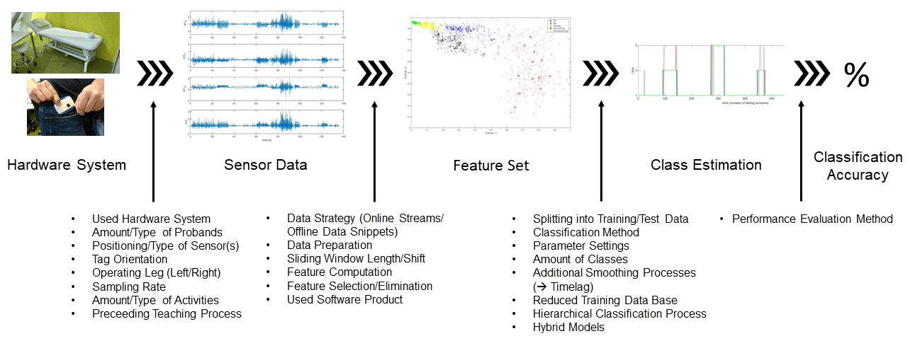
This study aims to be an advisor for creating classification models for HAR systems with wearable sensors and an additional help for finding optimal parameter settings. In Fig. 1, we depicted some influencing variables on the classification accuracy of a HAR system (see enumerations at the figure bottom). We split the influences according to their occurrence in the classification process. Most of these influencing variables have been studied in this work such as optimal window lengths and shifts, good features and how to select them, what is the minimal size for the training database, is a preceding teaching process necessary, and so forth. Figure 1 also shows that, due to the huge number of influencing variables, it is not easy to fully understand a classification process, and it is only related with much work. Therefore, the comparability between different classification tasks also becomes difficult.
The rest of the paper is organized as follows. Section 2 summarizes relevant work on human activity recognition. Section 3 explains the hardware and software infrastructure used in our HAR system and declares the used data collection processes. In the Sects. 4–6, results of our experiments with the three different hardware systems are presented and discussed. In Sect. 7, a short comparison of the best-reached classification accuracies with the different hardware systems is given. Finally, Sect. 8 concludes the paper.
In recent literature, smartphones often serve as a tool for implementing a HAR system (San Buenaventura and Tiglao, 2017; Nguyen et al., 2015; Büber and Guvensan, 2014; Ustev et al., 2013; Saha et al., 2017; Abdullah et al., 2020; Ashwini et al., 2020; Weng et al., 2014), as they are equipped with a rich set of sensors. However, device independence to remedy varying hardware configurations as well as efficient classifiers to prolong battery life and limit memory usage are still problems to be tackled.
Other challenges in the field of activity recognition are the differences in the way people perform activities concerning speed and accuracy (user independence) as well as the sensor positioning on the human body to find a position with high information gain and good separable features. Orientation independence of the sensor is also often desirable.
In Bloomfield et al. (2020), the difficulty of comparing HAR accuracy throughout literature is mentioned, since implementations vary across subject health or functional impairment, number of sensors and their placement locations on the body, activities performed, number and type of classes to distinguish, and validation techniques used. Additionally, various sensors may record with different measurement accuracies. For validating results of trained models, some papers use an n-fold process where samples from all subjects are blended. An alternative and better scheme involves the leave-one-subject-out (LOSO) technique so that the test set contains data of unseen subjects. In Kulchyk and Etemad (2019), classification accuracy drops from 100 % to 78.35 % when using the LOSO technique instead of splitting training and test data into 70 % : 30 % or using 10-fold cross-validation.
The optimal sensor placement on the human body plays an important role. Comparisons of different sensor positions have been considered in Kulchyk and Etemad (2019), Nguyen et al. (2015), Altun et al. (2010) and Saha et al. (2017). In Kulchyk and Etemad (2019) the ankle was the best sensor position, while in Nguyen et al. (2015) and Altun et al. (2010) the trouser side pocket and the right thigh, respectively, were the best choices. However, in Saha et al. (2017) the shirt pocket was better than the right trouser front pocket and two further sensor positions.
In our work, we have chosen the trouser pockets as a desirable unrestricted sensor position. In literature, we found some publications that also used this sensor placement (San Buenaventura and Tiglao, 2017; Nguyen et al., 2015; Büber and Guvensan, 2014; Ustev et al., 2013; Saha et al., 2017; Abdullah et al., 2020; Weng et al., 2014), in addition to multiple publications with other sensor positions. In Table 1, these publications are listed with additional information about type and placement of sensors, number of activities, used classification methods and their performance.
Bloomfield et al. (2020)Kulchyk and Etemad (2019)San Buenaventura and Tiglao2017Nguyen et al. (2015)Büber and Guvensan (2014)Altun et al. (2010)Ustev et al. (2013)Saha et al. (2017)Abdullah et al. (2020)Yang and Zhang (2017)Chuang et al. (2012)Ashwini et al. (2020)Mannini and Sabatini (2011)Weng et al. (2014)Table 1Some existing studies with emphasis on the sensor position “trouser pockets”.
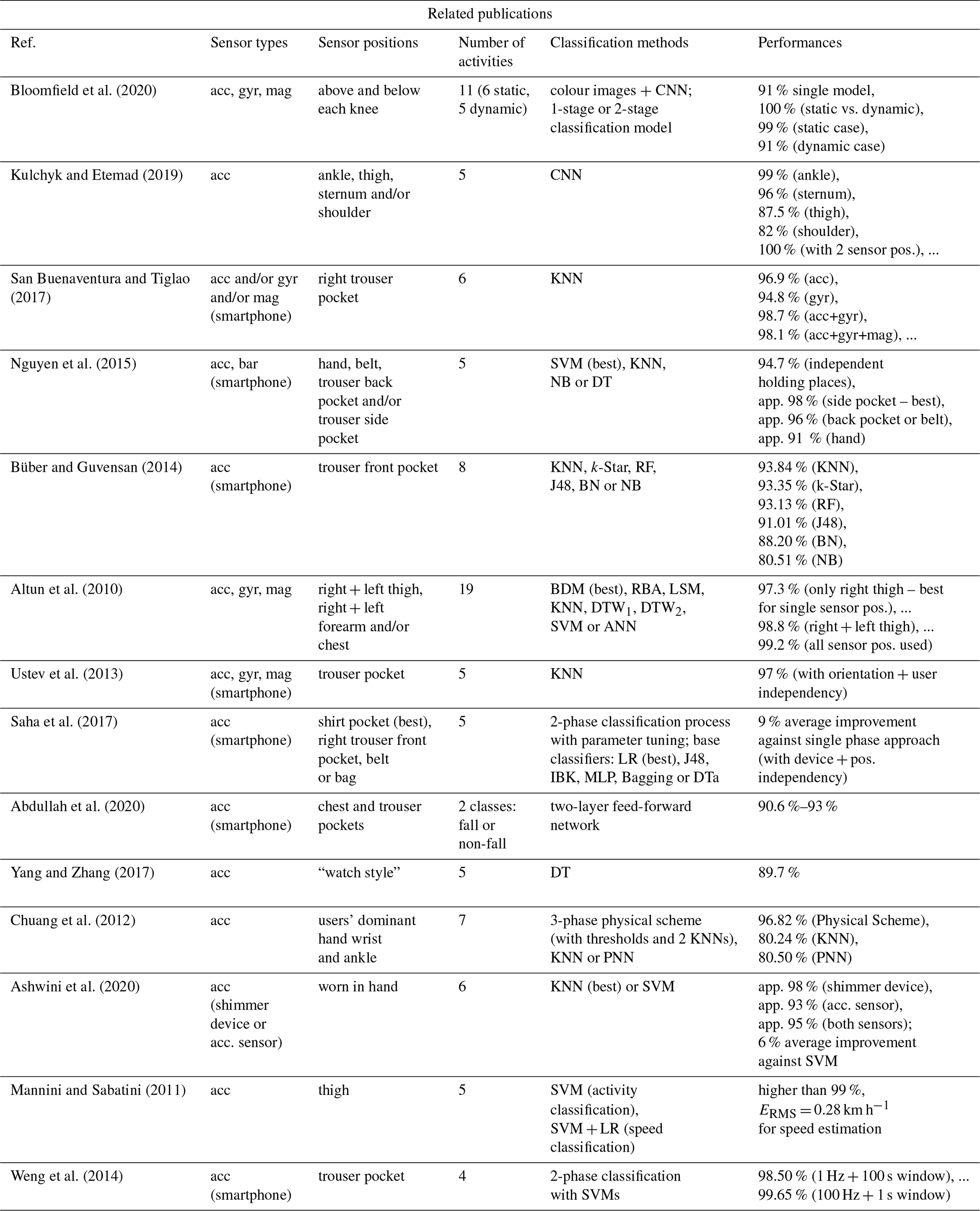
In Table 1, the following abbreviations are used: acc (acceleration), gyr (gyroscope), mag (magnetometer), bar (barometer), app (approximately), pos (position), CNN (convolutional neural network), KNN (K nearest neighbour), SVM (support vector machine), NB (naïve Bayes), DT (decision tree), RF (random forest), J48 (decision tree – J48), BN (Bayesian network), BDM (Bayesian decision-making), RBA (rule-based algorithm), LSM (least-squares method), DTW (dynamic time warping), ANN (artificial neural network), LR (logistic regression), IBK (instance-based classifier with parameter K; same as KNN), MLP (multi-layer perceptron), DTa (decision table), PNN (probabilistic neural network), ERMS (root-mean-square error).
Some publications listed in this table fixed the sensor at the thigh (Bloomfield et al., 2020; Kulchyk and Etemad, 2019; Altun et al., 2010; Mannini and Sabatini, 2011), and three further publications examined a sensor placement on the wrist similar to a watch (Yang and Zhang, 2017; Chuang et al., 2012) and in the hand, respectively, (Ashwini et al., 2020). Other sensor positions like ankle can be found in the column sensor positions. If the authors used smartphones for the data collection process, we added the word “smartphone” in the “Sensor types” column in brackets.
If we take a closer look at Table 1, it is apparent that the usage of a single sensor type (accelerometer) achieves good classification performance. In San Buenaventura and Tiglao (2017), the additional use of gyroscope and magnetometer data resulted in an improvement in performance of 1.2 %.
A further interesting fact of Table 1 is that the number of activities to be classified do not negatively correlate with the classification performance. Also, publications with a high number of daily living activities as Bloomfield et al. (2020) and Altun et al. (2010) gained comparable results in performance.
In literature, common classification methods are support vector machines as well as k-nearest-neighbour (KNN) approaches. In Nguyen et al. (2015) and Altun et al. (2010), SVMs achieved the best results; on the other hand, in Büber and Guvensan (2014) and Ashwini et al. (2020), KNN methods performed best. So, there is no overall method that performs best regardless of circumstances. In Bloomfield et al. (2020), Saha et al. (2017), Chuang et al. (2012) and Weng et al. (2014), the idea to use several stages for classification instead of a single model approach turned out to be advantageous. In Saha et al. (2017), for instance, a two-phase approach improved the overall system by 9 % on average, whereas a combination of several classifiers led to an improvement of 7 %. In Ustev et al. (2013), the use of linear acceleration (excluding the effect of gravitational force) combined with the conversion of accelerometer readings from a body coordinate system to earth coordinate system gave huge improvements in classification accuracy.
In the following, we want to summarize – for the particularly interested reader – the uniqueness, strengths and weaknesses for every paper listed in Table 1.
Bloomfield et al. (2020) described a wearable sensor system that is fixed above and below both knees. Data were logged at 25 Hz, which was sufficient to measure the lower extremities. A special approach to solve the problem of classification is the quaternion orientation representation of a body's orientation in three dimensional space. This information is transformed into colour images that serve as input for CNNs to get an automatic feature extraction. The LOSO validation technique was used. During data processing, it was found out that the body-worn sensors had slipped substantially on the legs of two subjects during cycling activities and on one subject during running activities. These trials had to be excluded from further evaluations. In this study, static tasks were better classified as dynamic tasks. The classification of data from subjects during cycling, ascending and descending stairs turned out to be difficult. Moreover, the different execution speeds of the subjects made it difficult to classify walking and running samples. Furthermore, the authors stated that battery lifetime would be better for single sensor systems using only accelerometers.
Kulchyk and Etemad (2019) proposed a system without the need for pre-processing, as they use an end-to-end solution via CNN only. They used a publicly available dataset and three validation techniques, also regarding the robust LOSO validation. They stated that the minimum number of acceleration sensors required for perfect classification accuracy is two, where at least one of the sensors should be located on a body part with a wide range of motion such as the ankle.
San Buenaventura and Tiglao (2017) made tests with lightweight classifiers (decision tree, KNN) while minimizing resource use. The KNN method, combined with data of accelerometer–gyroscope and a subset of eight features (found via the “ReliefF” feature selection algorithm), was sufficient for recognition. Frequency domain features were not necessary, as classifications with solely time domain features gave the best results. Accuracy also reduced slightly when a magnetometer was added to the accelerometer–gyroscope combination. For distinguishing upstairs and downstairs activities, the skewness feature of the accelerometer data was useful. For future analysis, additional physical and statistical features as well as other feature selection techniques would be interesting.
Nguyen et al. (2015) developed a HAR system that should perform robustly in any position that a smartphone could be held and which should be suitable for real-time requirements (sampling window size of 3 s). This goal was reached with an accuracy of more than 82 % for each activity in each of the four possible holding positions. The authors wrote that wearing multiple sensors on different body parts would be uncomfortable. The best results were achieved by SVM classifiers combined with the trouser side pocket. Furthermore, new features are extracted from a tri-axis accelerometer and a barometer like the variance of atmospheric pressure, and afterwards the features got normalized to a standard range of −1 to 1. So, they found features that are capable of distinguishing walking, ascending and descending stairs better than features of conventional methods. Moreover, the tracking of the subjects in a building completed the study. Nevertheless, analyses were only made with 10-fold cross-validation and with all 118 features.
Büber and Guvensan (2014) implemented a mobile application to report the daily exercises of a user to estimate calorie consumption. The system is energy-efficient, runs offline and has only 10 kB training data to be stored. The experiments showed that 10 instances of each activity class are enough to get the same accuracies with the best classifier (KNN method, K = 1). Six classifiers and two feature selection algorithms showed that 15 out of 70 normalized, time domain features are enough to get the best success rate. As the system had slight difficulties to classify ascending and descending stairs, the authors propose to combine these two classes, if possible, into one class. Points to be improved in future are the fixed location and orientation of the phone in the trouser pocket, the use of a 10 s windowing process and the sole use of the 10-fold cross-validation method.
Altun et al. (2010) made a comprehensive study that compares eight classification methods in terms of correct differentiation rates, confusion matrices, computational costs as well as training and storing requirements. The classifier BDM (Bayesian decision-making) achieved the highest classification rates with RRSS (repeated random sub-sampling) and 10-fold cross-validation, whereas the LOSO technique recommended SVM, followed by KNN (with K = 7). In this study, 19 activities were classified via acceleration, gyroscope and magnetometer readings of sensors placed on five different body places of eight young subjects. Sampling frequency was set to 25 Hz, and data were segmented into 5 s windows. A big feature set was reduced via principal component analysis from 1170 normalized features to 30. The utilized receiver operating characteristic (ROC) curves presented, in a very clear way, which activities are mostly confused. Also, the analysis made with reduced sensor sets as well as the long list of potential application areas of HAR systems is very interesting. Moreover, for future investigations, the authors propose the development of normalization between the way different individuals perform the same activities. New techniques need to be developed that involve time wrapping and projections of signals as well as comparing their differentials.
Ustev et al. (2013) specifically focused on the challenges of user-, device- and orientation-independent activity recognition on mobile phones. The orientation tests (same phone in vertical/horizontal orientation) especially showed that conventional HAR systems using phone coordinate systems are not robust enough. Firstly, Ustev et al. (2013) proposed to use time domain, frequency domain and autocorrelation-based features. Secondly, linear acceleration that excluded the effects of gravitational force increased the accuracy further. Thirdly, the switch to Earth coordinates further boosted the classification accuracies up to 97 %. The only drawback of this method is the higher energy consumption for using three sensors, which will be further investigated by the authors.
Saha et al. (2017) used simple time domain features, such as the mean of the logarithm of each acceleration axis, to implement a two-phase activity recognition system which is device independent as well as position independent. Therefore, six different smartphones and four different positions of the devices are used. It is shown that the pattern for one activity varies from one device to the other, which makes, for example, threshold-based approaches unsuitable. Noise and outliers were eliminated, and filtering was conducted to preserve medium-frequency signal components. Phase 1 of activity classification chooses the best training dataset that yields maximum overall accuracy for a test set. Phase 2 further improves the accuracy by condition-based parameter tuning of a given classifier. As shirt pocket was found to be the best position for collecting training data, training data were only collected with this specific position.
Abdullah et al. (2020) tried to distinguish fall and non-fall events by computing four time domain features from accelerometer data and by using a two-layer feed-forward network. Data are collected at two different carrying positions of the smartphone; 26 fall and 41 non-fall events were classified with 93 % accuracy. In future, this study should be further extended to more subjects (now 2), to a bigger feature database and to more classifiers.
Yang and Zhang (2017) used a wearable device in a watch style for classifying five daily activities with an acceptable accuracy. A big advantage is the comfortable way of wearing the sensor. Unfortunately, sitting or bicycling activities cannot be detected reliably. For pre-processing, a median filter for eliminating noise and a temperature sensor for correcting the acceleration data were used. Afterwards, several time domain and frequency domain features were computed, and a decision tree was applied. To be more energy efficient, the micro-controller was set to a sleeping mode and only woke up when necessary. Weaknesses of the analyses are that only young people participated in the study, and the classification decision tree was only created from data of all persons together. Furthermore, analyses including feature selection methods or other classifiers would be interesting.
Chuang et al. (2012) applied a divide-and-conquer strategy for first differentiating dynamic activities from static activities (threshold-based), and then posture recognition was used to classify the static activities sitting and standing. Therefore, thresholds for pitch and roll angles of the ankle were used. For dynamic activities, the exercise classification algorithm classified them into three classes: running, cycling and ambulation activities. Afterwards, the ambulation classification algorithm was utilized to distinguish between level walking, walking upstairs and walking downstairs. Here, two KNN classifiers with K = 5 were used for pre-processed (high-pass filtering) and transformed signals (13 time domain and frequency domain features). The LOSO cross-validation method confirmed the successful recognition of seven activities with 96.82 %. The use of two acceleration sensors, worn on the participant's ankles and wrist, was a good decision. The only drawback of the analysis could be the participant's limited age range between 20 and 25 years.
Ashwini et al. (2020) presented a classification system for six different hand gestures, where the subjects carry a sensor in the hand. They compared two sensors (shimmer sensor versus tri-axial accelerometer sensor) with 38 healthy subjects, pre-processed data, eight features and two different classifiers (SVM and KNN). Improvements were achieved upon considering both shimmer and accelerometer data. Among the classifiers considered, KNN had an average accuracy around 6 % better than SVM. Unfortunately, the LOSO validation was not considered, and the exact pre-processing strategy was not explained.
Mannini and Sabatini (2011) showed that online human activity recognition (1 s time windows) with one acceleration sensor mounted at the right thigh is possible for five activities with high accuracies. Even with the LOSO technique, results as high as 92 % could be achieved. Furthermore, locomotion speed was estimated for the classified activities walk and run. Overall, two SVMs fulfilled these tasks, and six young subjects participated in the study.
Weng et al. (2014) tried to develop a HAR system with high accuracy and low power consumption. Therefore, studies with 1 Hz sampling rate and long time windows were conducted and showed very good results for four activities and three young men. To classify two static and two dynamic activities of daily life, three SVMs had been used in a hierarchic manner to classify low-pass-, mean- and median-filtered acceleration signals. In future, more participants and real-life environments should be analysed. Drawbacks of the method are the small number of activities and the huge time windows, as the width of the time windows had to be increased when sampling rates decreased.
In general, HAR systems with wearable sensors achieve good performance. So, it is worth it to further investigate such systems to remain competitive and to produce further improvements to pave the way for future technologies.
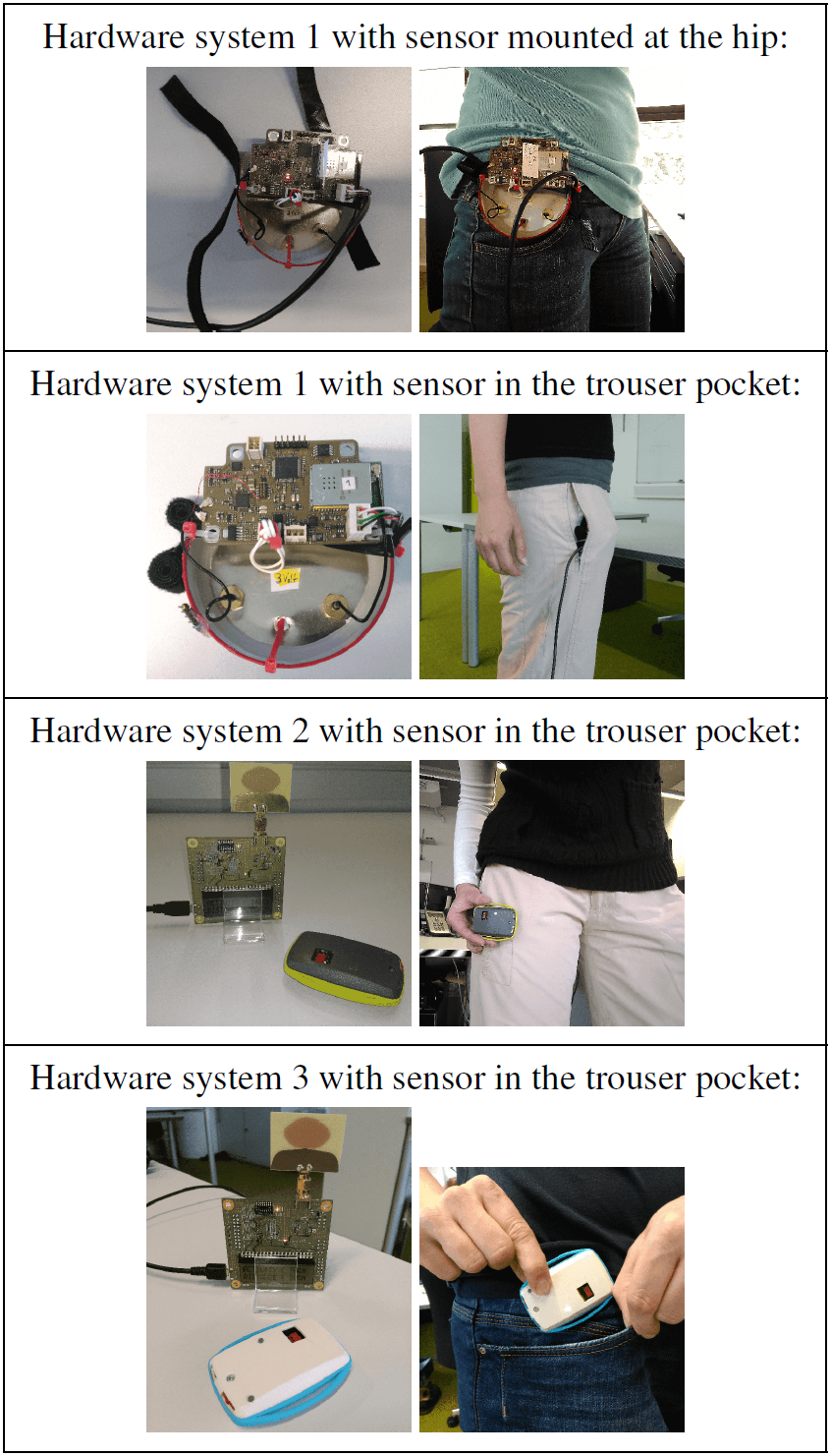
For data collection, three different hardware systems have been used, as there have been multiple enhancements during the classification analysis. For system 1, a customized data acquisition system with acceleration sensor ADXL335 and micro-controller PIC32MX695F512H has been used. The data are transferred via LAN cable to the PC. So, the orientation and rotation of the sensor is restricted during carrying in the trouser pocket. For system 2, we used a Decawave EVK1000 evaluation kit with micro-controller STM32F105xx as base station. Additionally, a self-built tag with a LIS3DH acceleration sensor and a STM32L051x8 micro-controller was utilized. The data are transmitted via radio wave from the tag to the base station and transferred via LAN cable to the PC. System 3 is nearly the same as system 2, but instead of the LIS3DH acceleration sensor an IMU LSM9DS1 was used to record acceleration and gyroscope data. Table 2 shows photos of the different systems. We recorded accelerometer data with 1 kHz using system 1, accelerometer data with 50 Hz using system 2, and accelerometer and gyroscope data with 59.5 Hz using system 3. During the analysis with system 1, we concluded that even 20 Hz would be enough for good results; therefore, we reduced the sampling rate with progression of hardware development.
Within the experiments with systems 1 and 2, one healthy (self-assessed) female person was used for data generation. For analysis with system 3, 12 healthy people (5 female, 7 male) served as subjects. The subjects decided by themselves how the sensor was to be initially put in the pockets of the trousers and how fast or clear each activity was to be performed.
In our analysis, we tested various movements such as toe tip, heel tip, swivelling hips, stamping with feet, moving the knee up and down, or moving the knee left and right for sufficient recognition. Finally, we decided that the therapy table should move upwards when the masseur moves the knee up and down such as using an air pump. The toes are kept on the ground during the pumping process. Otherwise, the therapy table should move downwards, when the masseur moves the knee left and right with the toes kept on the ground. If the masseur is doing anything else, such as standing, giving a massage, going or running, the therapy table should remain in its current position.
For data collection, three classes of movements have been recorded with five different activities:
-
Class 1 was go, run or massage.
-
Class 2 was pump therapy table up.
-
Class 3 was pump therapy table down.
In the next sections, this data material is referred to as “offline data”. If we make use of this offline data during analysis (e.g. for feature selection processes), then we split these data into 70 % training data samples and 30 % test data samples and make a cross-validation with 1000 different choices of training data samples collected from the whole dataset.
Furthermore, we recorded data streams (called “online data” in the next sections) with the following sequence of activities:
- 1.
go – class 1 for 25 s,
- 2.
pump up – class 2 for 10 s,
- 3.
massage – class 1 for 25 s,
- 4.
pump down – class 3 for 10 s,
- 5.
go – class 1 for 10 s,
- 6.
run – class 1 for 10 s,
- 7.
go – class 1 for 5 s,
- 8.
pump up – class 2 for 5 s,
- 9.
massage – class 1 for 20 s,
- 10.
pump down – class 3 for 5 s,
- 11.
massage – class 1 for 10 s.
In Fig. 2a, an example of an online data stream is depicted. First, acceleration data for each axis (accX, accY, accZ) are shown. The last panel shows the acceleration magnitude computed as acc .
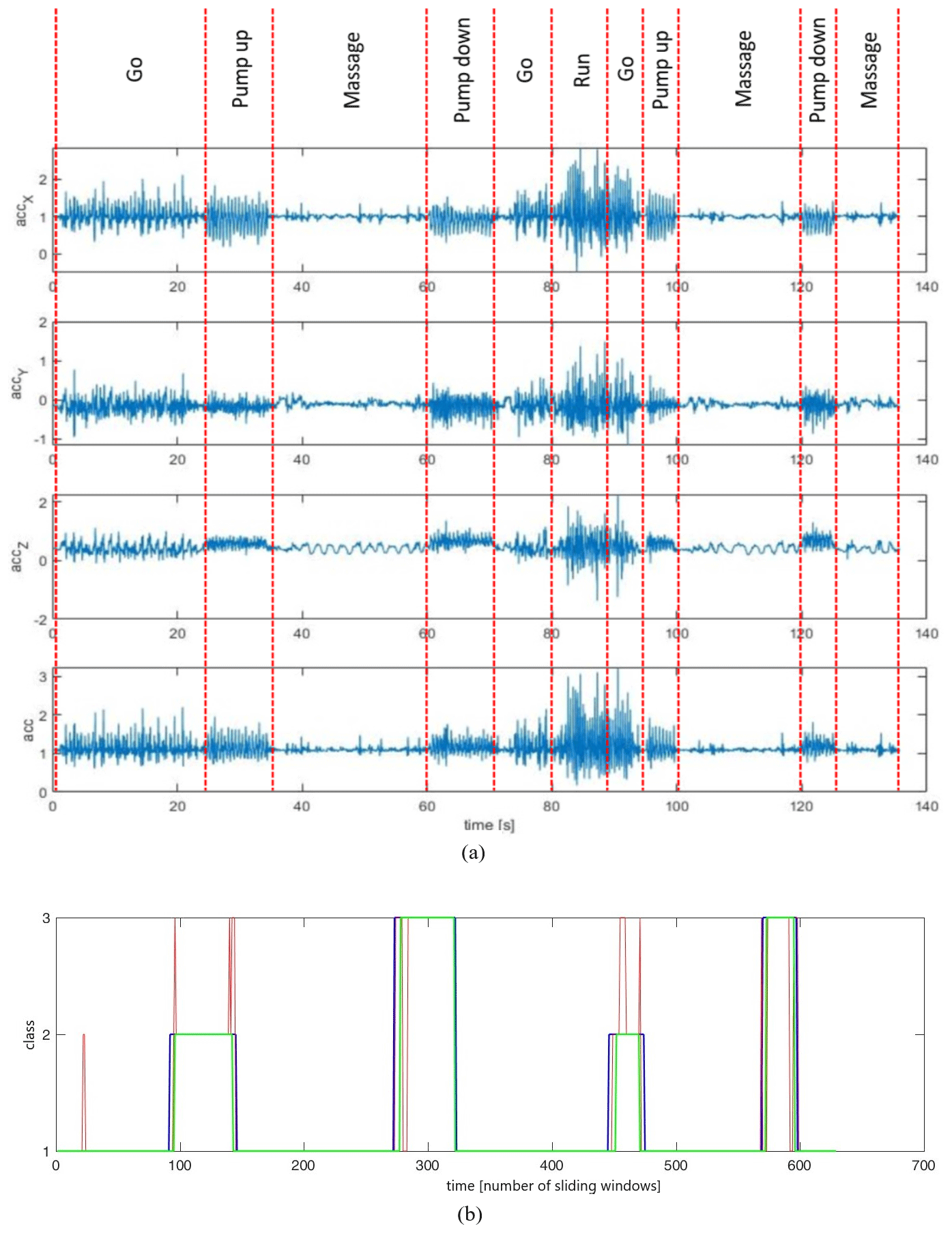
Figure 2Acceleration data and the estimated classes of an exemplary online data stream. (a) Acceleration data; (b) estimated classes without (red line) and with smoothing (green line); blue line represents ground truth.
As a tool for our analysis, we used MATLAB without any special toolboxes for classification purposes.
In the data pre-processing step, the data are segmented into windows of 3 s, and these windows are computed every 200 ms out of 10 online data streams of one subject (test data). For training, 55 samples of each kind of activity are used from a separate recording with the same subject. Therefore, class 1 consists of more training data as classes 2 and 3 as there are more different movements in it. In detail, we chose an approach with classification into five classes followed by a renaming of classes 1–5 to new classes 1–3. For the execution of the two different pumping exercises, the same leg, as where the sensor was mounted or pushed into the pocket, was used. After segmentation, multiple features are generated and normalized to values between 0 and 1.
For the acceleration data of each axis as well as acceleration magnitude, 43 features are computed, which are short-time energy (STE), short-time average zero-crossing rate (ZCR), average magnitude difference (AMD), root-mean-square energy (RMS), 15 specific band energies (BE1–BE15), spectral centroid (SCENT), median of peak differences (PEAKDIFF), number of peaks (PEAKS), spectral roll-off (SROLL), spectral slope 1 (SSLOP1), spectral slope 2 (SSLOP2), spectral spread (SSPRE), spectral skewness (SSKEW), spectral kurtosis (SKURT), spectral bandwidth (SBAND), spectral flatness (SFLAT) and the first 14 mel-frequency cepstrum coefficients (MFCC-1 to MFCC-14). In summary, we have 172 features of which 3 × 4 are of the time domain, 26 × 4 are of the frequency domain and 14 × 4 are out of the cepstrum. Further information about our used features and additional features can be found in most of the articles in our reference list (Antoni and Randall, 2006; Bajric et al., 2016; Beritelli et al., 2005; Fernandes et al., 2018; Gupta and Wadhwani, 2012; Morris et al., 2014; Nandi et al., 2013; Preece et al., 2009; Prieto et al., 2012; Rosso et al., 2001; Shen et al., 2013; Singh and Vishwakarma, 2015; Yi et al., 2014; Zhang et al., 2013).
For evaluation of different machine learning applications, we collected many features in a database that could be reasonable for such purposes. Afterwards, with feature selection or elimination processes, we automatically find a suitable subset of features. For our daily work with different classification tasks, this prefabricated feature-based approach will reduce our time for future analyses. In another publication (Pichler et al., 2020), we also used various features to analyse vibration data of bearings. In Capela et al. (2015), also a huge list of features is generated.
For classification, we used the one-nearest-neighbour (1NN) method, as in our literature study KNN methods reached classification accuracies that were as good as other methods, such as CNN. In Büber and Guvensan (2014) and Ashwini et al. (2020), the KNN method performed even better compared to other classic approaches for classification. For our application, it is important to quickly get a classification response for motor control. Therefore, we decided to use an easy and comprehensible method, and, according to the literature research, it is also comparably as good as other approaches.
Using the 1NN method, for each test data sample the most similar training data sample is searched, and the class of this training data sample is assigned to the test data sample. Additionally, a smoothing process is used to overcome the problem of individual false assignments. For this idea, a time window of length 4 s is moved over the classification results of the data stream. The most commonly estimated activity class within this period is then the new activity class for the timestamp at the middle of the time interval. This results in a time lag of 2 s for online execution until the final class is certain. In Fig. 2b, an example is given for the classification results of an online stream with and without smoothing. The red line shows the estimated classes without smoothing, the green line shows the estimated classes with smoothing and the blue line is the correct result.
We computed for each feature the ability to classify between the three classes. Remarkably, the features computed from acceleration magnitude, acc, and from acceleration of the z axis, accZ (accZ shows horizontally forward), performed best for the hip sensor position. The best feature (SBAND computed from acc) reached 81.42 %. For the trouser pocket sensor position, features computed from acc and accX performed best. The best feature was MFCC-4 of acc with 95.22 %. The worst features for both sensor positions reached 33.33 %.
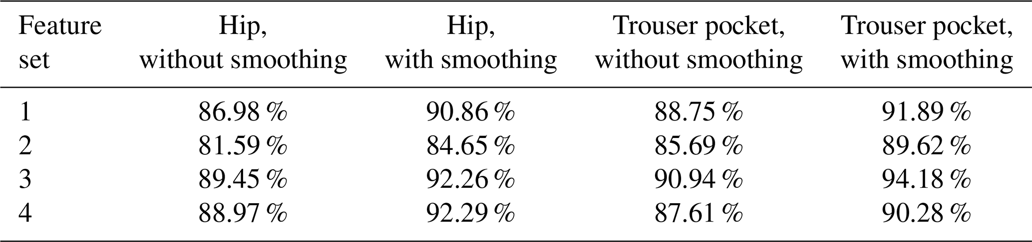
Furthermore, we compared the two different sensor positions (hip and trouser pocket) with different sets of features:
-
Feature set 1 was 172 features
-
Feature set 2 was 43 features of acceleration magnitude
-
Feature set 3 was a combination of 23 features that had the highest ability to separate the different classes on its own (with the hip sensor position)
-
Feature set 4 was a combination of 30 features gained by the backward elimination process (with the hip sensor position)
The backward feature elimination process was used to find a small subgroup of features with ample information content. The process starts with all features and then successively eliminates features, such that the classification accuracy is maximized in each elimination step (Kim et al., 2006; Meyer-Baese and Schmid, 2018).
In Table 3, the classification accuracies for the different feature sets with and without using an additional smoothing process are illustrated. On the basis of the results in Table 3, the activities “pumping the therapy table up/down” are best recognized with positioning the sensor in the trouser pockets. With the use of hardware system 1, the sensor is restricted in its movement within the trouser pocket. So, it behaves similarly to a sensor mounted at the thigh. Moreover, we can see in Table 3 that an additional smoothing process is advantageous if the classification results do not have to be available immediately. Furthermore, the use of an optimal feature set is important, and the features resulting from acceleration magnitude also performed good without a significant drop in acceleration accuracy.
Table 3Comparison of classification accuracies for different sensor positions with hardware system 1 and online data.
In our analysis, we also performed a backward feature elimination process for feature sets 1 and 2 with the trouser pocket sensor position. Figure 3 shows the theoretical accuracies within the feature elimination processes with the use of offline data.
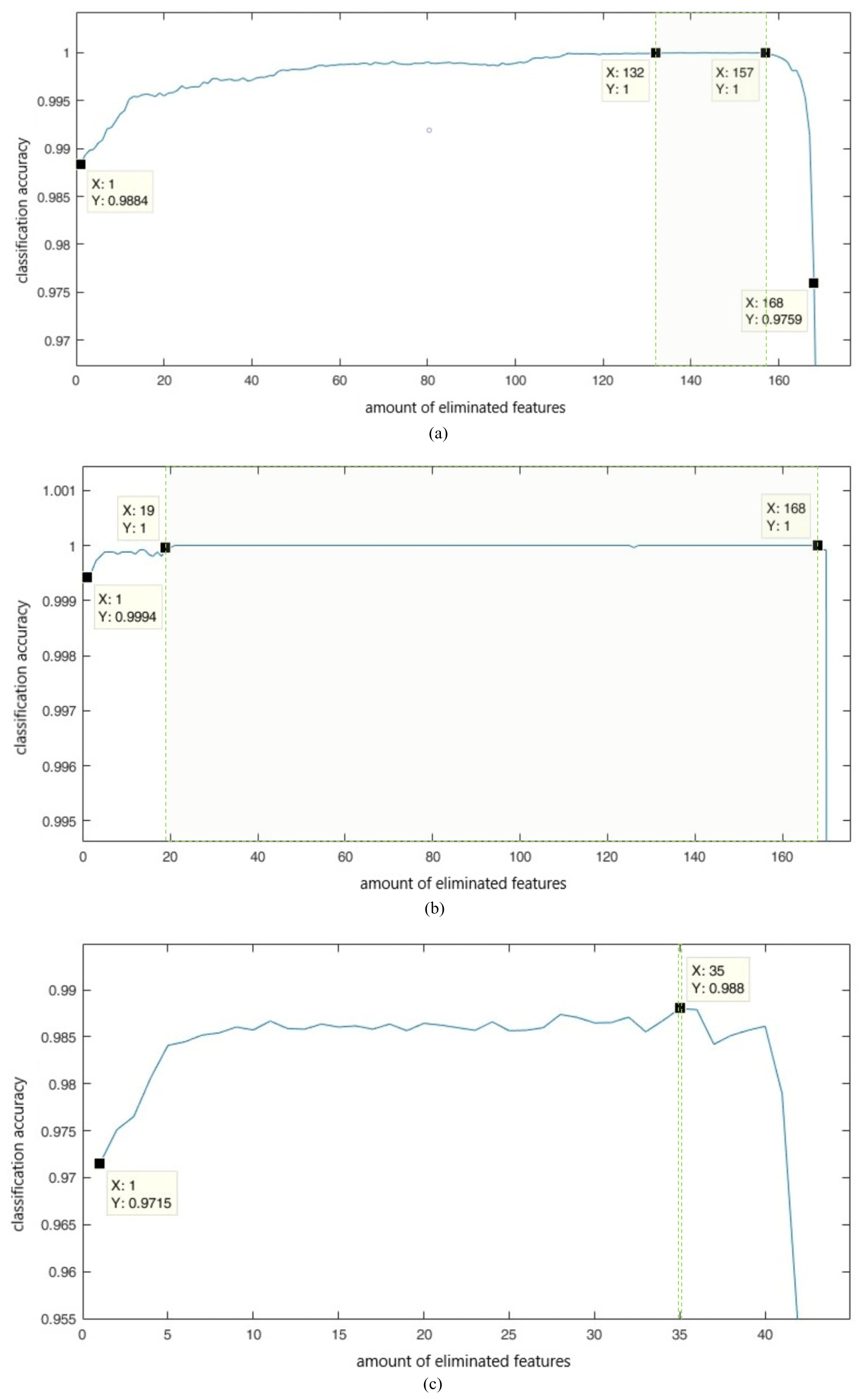
Figure 3Progress of classification accuracy during the backward elimination process. (a) 172 features, hip sensor position, offline data; (b) 172 features, trouser pocket sensor position, offline data; (c) 43 features of acc, trouser pocket sensor position, offline data.
The data within a window of offline data streams include only data of one special activity, which may explain the improved performance.
In Fig. 3a, a set between 15 and 40 features gains a perfect classification result. In Fig. 3b, a set between 4 and 153 features gains 100 % classification accuracy. Therefore, the trouser pocket sensor position needs fewer features to perform well on the training set. If we use feature set 2 as the initial set for the backward elimination process with data gathered from the trouser pocket sensor position, the classification accuracy is highest with eight features (98.8 %, see Fig. 3c). These eight features are MFCC-4, SBAND, BE4 (64.95–135.93), BE3 (31.75–64.95), MFCC-6, MFCC-13, MFCC-14 and MFCC-8. The cepstrum coefficients performed especially well. With these eight features, we computed the classification accuracy again for online streams as in Table 3. For the trouser pocket sensor position and no smoothing, we attained an accuracy of 89.77 %. For the same conditions with smoothing, we obtained 93.95 %.
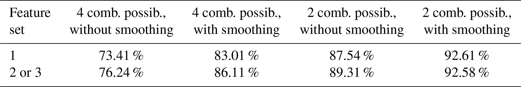
Next, we examined the decrease in classification accuracy if we add all four possible combinations of leg movement and sensor positioning in the trousers. We recorded data with the sensor placed in the right trouser pocket, and leg movements are fulfilled with the right or left leg. Additionally, we recorded data with the sensor placed in the left trouser pocket, and leg movements are made with the right or left leg. The training data arise from 240 windows of 3 s of each activity group with four combination possibilities and 119 windows of 3 s of each activity group for two combination possibilities. As test data, we used 20 online streams of one subject for four combination possibilities, and 10 online streams of one subject for two combination possibilities (five online streams of each combination possibility have been recorded). For comparison purposes, we used three feature sets:
-
Feature set 1 was 43 features of acceleration magnitude
-
Feature sets 2 and 3 were a combination of 23 and 9 features, respectively, gained by backward elimination processes
Feature set 2 is attained by a backward elimination process started with 43 features of acceleration magnitude and all four combination possibilities of leg movement and sensor positioning. Feature set 3 also results from a backward elimination process started with 43 features of acc but with only two combination possibilities – leg movements and sensor positioning must be at the same side. In Table 4, feature set 2 is used for columns 2 and 3, whereas feature set 3 is used for columns 4 and 5. The abbreviation “comb. possib.” is used for the term combination possibilities. Table 4 demonstrates that with complete freedom with respect to the choice of dominant leg and trouser pocket, the classification accuracy falls from 94.18 % to 86.11 % for the best feature set with smoothing. With the restriction that the leg movements pumping up/down and the trouser pockets must be on the same side, 92.61 % can be achieved. In conclusion, it is important that the key movements for pumping the therapy table up or down are performed with the same leg as where the sensor is positioned. This can be observed in particular with classification results without an additional smoothing process.
Table 4Classification accuracies with freedom about choice of dominant leg or trouser pocket with hardware system 1 and online data.
In the next step of our analysis, we examined the impacts of a change in sampling rate. We simulated different sampling rates with the function decimate in MATLAB. First, we consider offline data with 83 data samples of each kind of activity for training and 36 data samples of each activity for testing. We used, again, windows with a length of 3 s, the 1NN method, 43 features of acc and the requirement that key movements of each leg must be at the same side as the sensor position. If we consider the black line in Fig. 4a, we recognize a decimation in classification accuracy with 10 Hz or less. The best choice would be 20 Hz. The pumping down activity was estimated best (blue line).
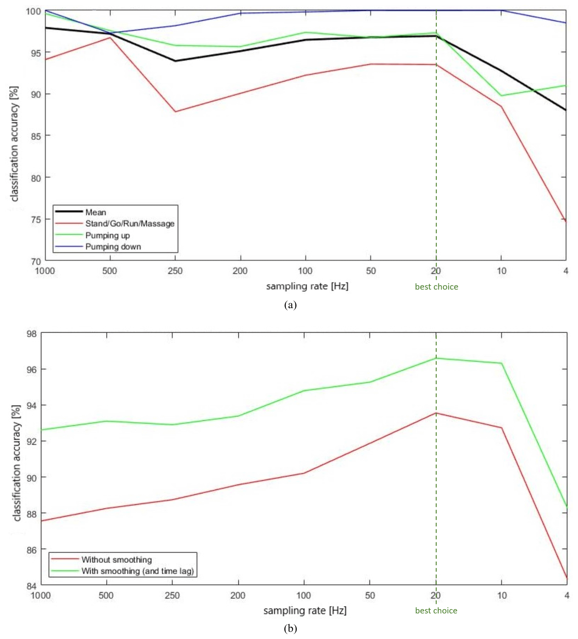
Figure 4Modification of classification accuracy with different sampling rates. (a) Offline data; (b) online data.
Furthermore, let us consider the same evaluation for 10 online data streams as test data and 119 samples of 3 s for each class as training data. Figure 4b shows the result. For our online data streams, 20 Hz is also the best choice. With an additional smoothing process, the classification accuracies raise from 92.61 % with 1 kHz to 96.59 % with 20 Hz. These results are obtained with the sole use of acceleration magnitude, acc, for feature computation. If we start a backward feature elimination process with all 43 features of acc, we end up with a best feature set consisting of 15 features and an accuracy of 96.58 %. So, also with 15 features and 20 Hz sampling rate, the level of performance remains the same. If we use all 172 features from accX, accY, accZ and acc as well as 20 Hz sampling rate, we get 98.23 % with smoothing. In conclusion, a sampling rate of 20 Hz is recommended here, and a sampling rate of at least 10 Hz is needed for an acceptable performance of the HAR system.
Additionally, we studied the effects on classification accuracy of different window lengths that segment our data streams. For this purpose, we fix the sampling rate to 20 Hz and vary the window lengths between 0.5 and 4.5 s. Attention should be paid to the fact that we have 726 data samples per activity for 0.5 s windows and 78 data samples per activity for 4.5 s windows, as the overlapping of the windows of 50 % was kept fixed. As in the last paragraph, we consider the corresponding figures for offline and online data analysis (same test and training data; 43 features computed out of acc). Figure 5a shows that long, sliding time windows are preferable – with a significant drop for windows shorter than 1.5 s.
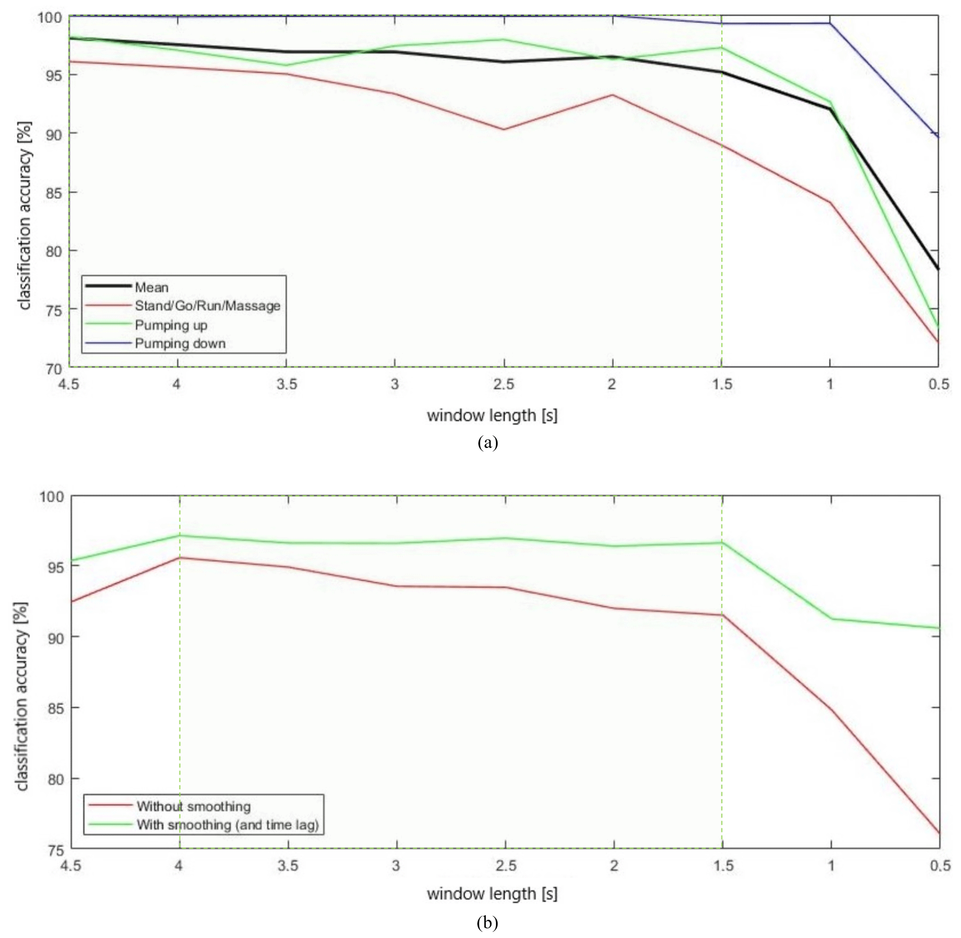
Figure 5Modification of classification accuracy with different lengths of sliding time windows. (a) Offline data; (b) online data.
If we consider online data streams for test data as in Fig. 5b, it does seem preferable to choose medium-sized windows. For a window length of 4.5 s, performance drops again, which we attribute to a recognition drop for short activity periods. If we choose a sampling rate of 20 Hz and a window length of 2 s, we get a classification accuracy of 91.99 % without smoothing and 96.39 % with smoothing as well as the acceptance of an additional time lag of 2 s. If we choose a sampling rate of 10 Hz and online streams for classification, we would need a window length of at least 2.5 s, as performance would drop from 95.14 % to 90.15 % with the use of 2 s windows and smoothing.
Furthermore, we made a short comparison with other classifiers – HMM (Rabiner, 1989), SVM (Chang and Lin, 2011) and a change point detection method – with 20 Hz and two different feature selection sets, but as these methods provided similar results with less than 1 % deviation for HMM and SVM and worse results for the used change point detection method, we stuck with the KNN methods. The coarse description of the used change point detection method is as follows. Firstly, on the basis of variances, change points are searched. Secondly, we look at the residence time in the foregoing state to avoid, untimely, state transitions. Thirdly, with the features of the time window after the change point, the new state is declared.
One big advantage of KNN methods is the easy realization and good comprehensibility. Also, a switch to the 5NN method instead of the 1NN method does not gain better results. So, we used K = 1 as in Büber and Guvensan (2014).
For our studies in this section, we used a new hardware system – see also hardware system 2 in Sect. 3. One subject made records with a tri-axis accelerometer with a sampling rate of 50 Hz and acceleration data limited within a range of ±2 g gravity. As in Sect. 4, three classes are used. Class 1 consists of 1614 data samples with activities “go”, “run” and “massage”, class 2 consists of 538 data samples for the activity “pumping the therapy table up” and class 3 consists of 538 data samples for the activity “pumping the therapy table down”. In this section, the sensor is placed into the pocket of the dominant leg (the leg that executes the key movements for classes 2 and 3). So, 50 % of the data are recorded with the sensor in the right pocket of the trousers and making the key movements for pumping the therapy table up or down with the right leg. The other 50 % of data are recorded with the sensor in the left trouser pocket and with a dominant left leg. Again, we use the 1NN method as classifier and features were computed from acceleration magnitude, acc. Due to the conducted feature engineering process, the list of features was adjusted to STE, short-time average zero-crossing rate of signal minus 1 (ZCR1), short-time average zero-crossing rate of signal minus 1.3 (ZCR2), AMD, RMS, eight specific band energies of spectrum (BE1–BE8), SCENT, median of peaks in spectrum (SPEAKS), SROLL, SSLOP1, SSLOP2, SSPRE, SSKEW, SKURT, SBAND, SFLAT and spectral flux (SFLUX). Features 1–4 are from the time domain, and features 5–25 are from the frequency domain. In this section, we did our analysis without cepstrum coefficients, as we wanted to find an easy lightweight method for classification with a low computational complexity. We set the window length to 2.88 s (144 data points) and shifted the windows every 0.32 s (16 data points). For the results with an additional smoothing process, we used only the last two classification estimates to form a new one (but with more weight for class 1). So, if there are two estimates with classes 1 and 2, we still remain in class 1. If there are two estimates with classes 2 and 3, we choose class 2 as the preferred class.
With these 25 normalized features, a forward feature selection as well as a backward feature elimination process was started for the above-mentioned offline training data of this section. These processes quickly find a local optima in contrast to brute-force methods where all parameter combinations are tested. The forward feature selection process starts with a feature, for which the maximum classification accuracy is obtained (and is easy to compute if there are more possibilities), and then successively adds a further feature, such that the classification accuracy is as high as possible (Kim et al., 2006; Meyer-Baese and Schmid, 2018).
In Fig. 6a and b, the progress of classification accuracy can be seen for adding features and eliminating features, respectively.
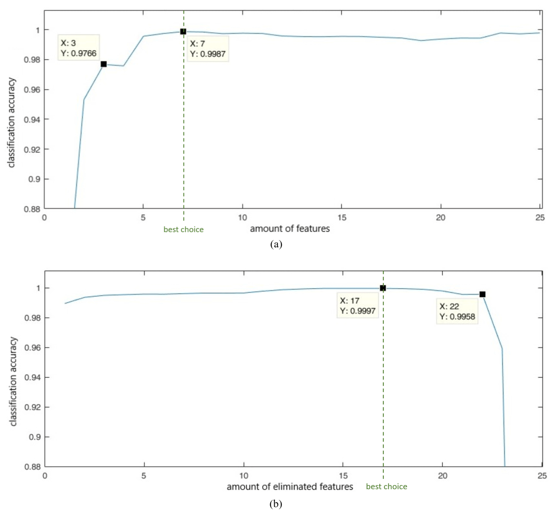
Figure 6Progress of classification accuracy during elimination processes with offline data. (a) Forward selection process; (b) backward elimination process.
Figure 6a shows that with only three features a good classification can be achieved but with seven features the best result is achieved (99.87 %). These specific features are BE1, SFLAT, SFLUX, RMS, BE4, BE5 and BE6. Figure 6b depicts that three features are enough for a good accuracy (99.58 %) but with eight features an accuracy of 99.97 % is possible. These features are BE3, SBAND, BE2, SFLAT, BE4, SSLOP1, SKURT and BE1.
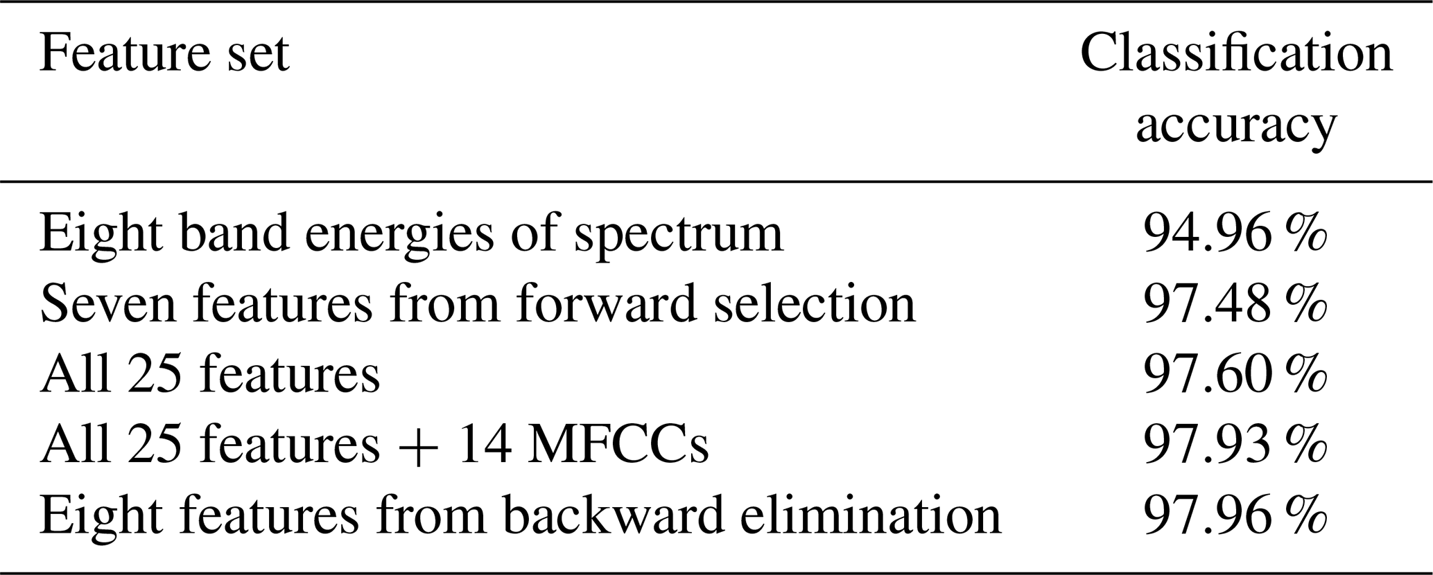
In a next step, we made a parameter optimization for these two specific parameter selections regarding window length, window shift and time lag of the smoothing process. Therefore, we used 10 online streams as test data and the offline data as training data. Interestingly, we already used an optimal combination of window length (2.88 s), shift (0.32 s) and time lag (0.32 s) for an additional smoothing process. With these parameter settings, we calculated the classification accuracies for five different feature sets, which are listed in Table 5. There, the eight features found via the backward elimination process achieved the highest performance.
Table 5Classification accuracies for different feature sets and online data.
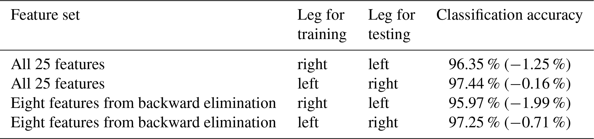
Another interesting question is whether training data recorded with one dominant leg are enough for control of the system with both legs. The results are posted in Table 6 for two different feature sets. If we change the dominant leg for training and testing for the same person, the performance does not drop significantly. So, if desired, training with one leg is enough for operating the system with both legs.
Table 6Classification accuracies for changes in dominant leg with online data.
During the next study, we made recordings with changes in the initial orientation of the tag in the trouser pockets as well as changes in how the base station is positioned on the table in front of the subject. We made four recordings with the four different possibilities of how the tag is placed into the pocket. Then we reversed the base station and made, again, four recordings with the four different tag orientations. All in all, the classification accuracies barely varied (between −1.13 to +0.51).
Finally, we studied how different parameter values, K, of the KNN classifier affect the classification accuracy. Up to now, we used K = 1 for hardware system 2, but now we also consider higher parameter values (K) when using eight features derived from backward elimination and how the classification accuracy will change. Therefore, we show for the best scenario of Table 5 the corresponding figure with alternating K. As we can see in Fig. 7, K = 1 or K = 3 would be a good choice. So, it practically does not matter if you choose K = 1 or K = 3.
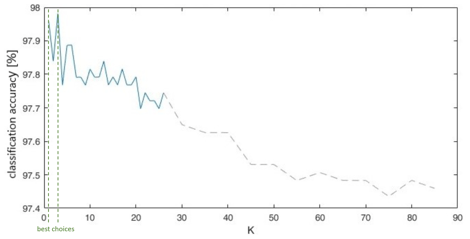
Figure 7Influence of parameter K of KNN classifier on classification accuracy with online data.
In this section, we switched to another hardware system, denoted as hardware system 3 in Sect. 3, and we made recordings with 12 subjects (5 female, 7 male). The height of the participants ranged from 1.65 to 1.86 m, with the location of the sensor placed in the pockets and varied between groin and a deep position at the thigh. Also, the initial orientation of the sensor in the pockets and varied at random. Furthermore, the subjects decided which leg to use for controlling the therapy table (only restriction: leg which records the signals must be the same as the leg for control). The clarity and pace of movements also varied between the different subjects.
We recorded data with a tri-axis accelerometer and a tri-axis gyroscope with a sample rate of 59.5 Hz. As in Sects. 3 and 4, offline and online data were recorded. The recorded offline data streams (used for training) have a length of 30 s for each activity group and subject. The five activities are go, run, massage and two key movements that imitate the operation of a foot pump (knee pumps in vertical or horizontal direction). The first three activities are collected in their own class. The online data streams with various activities (used for testing) consist of three runs of a length of 2 min and 15 s for each subject as listed in Sect. 3. Additionally, we made records of five further possible movements for controlling the therapy table. So, the offline data streams have been extended with the following activities: stamping, toe-tipping, describing a circle with the knee, swinging the hips left and right, and quickly moving the knees forward and backward in an alternating manner.
6.1 The used classification process and finding the best method
The procedure of the applied data-based classification is as follows:
-
Creating a training database. We computed several features out of raw signal sections of length 128; afterwards we normalized the features to values between 0 and 1.
-
Application of the classifier. We extracted training data samples of length 128 (with an shift of 32 for online data streams), computed and normalized the corresponding features, and made a comparison to the features of the training database for finding the best-suited class. Please make sure that test data samples are not contained in the training database.
The analysis took place as follows.
6.1.1 The used features
For classification, we used 59 features computed from data of the acceleration sensor as well as gyroscope sensor; 57 features are based on the magnitude, acc , as the orientation of the sensor in the trouser pockets is irrelevant. Features 58 and 59 are intuitive features that use information of the single axes and the force of gravity. Casually speaking, feature 58 computes the energy of acceleration in the direction of the force-of-gravity vector (scalar product of acceleration and gravity vector). On the contrary, feature 59 computes the energy of acceleration in the orthogonal direction to the force-of-gravity vector (use of cross product instead of scalar product). For gyroscope data, scalar and cross products are computed from the mean angular velocity and the current angular velocity.
Features 1–26 are out of the time domain: STE, ZCR1, mean level signal crossing rate (MCR), AMD, mean, variance, median, mean absolute deviation (MAD), minimum, maximum, range, interquartile range, 25th percentile, 75th percentile, skewness, kurtosis, harmonic mean, magnitudes of jerk, coefficient of variation (CV) or relative standard deviation (RSD), RMS, square root of the amplitude (SRA), crest factor (CF), impulse factor (IF), margin factor (MF), shape factor (SF), and kurtosis factor (KF). Features 27–57 are out of the spectral domain: root-mean-square energy (SRMS), eight specific band energy's of spectrum (SBE1–SBE8), SCENT, median of peak differences in spectrum (SPEAKDIFF), SPEAKS, SROLL, SSLOP1, SSLOP2, SSPRE, SSKEW, SKURT, SBAND, SFLAT, SFLUX, dominant frequency of signal, frequency centre (FC), root variance frequency (RVF), and seven symptom parameters. Features 58–59, as described in the last paragraph, are also out of the time domain.
6.1.2 The used classification method
The normalized feature vectors are assigned to a special class via the one-nearest-neighbour method, as this method provided good results in the foregoing studies, has a good comprehensibility and is easy to implement.
6.1.3 Possibilities for the computation of the classification accuracy
As in Sects. 3 and 4, we differentiate between online and offline data. The approach with offline data is detailed as follows:
-
For each subject and class, we have 50 data samples (raw signals).
-
For each class, 150 data samples of three subjects are used for training, and 450 data samples of nine subjects are used for testing.
-
We used cross-validation to get different selections of subjects for training and test data.
-
We computed a mean classification accuracy out of 220 results of cross-validation.
Details for the approach with online data are the following:
-
For training, data samples of the offline approach are used from all subjects. Later in Sect. 6.2, other configurations with less subjects are also analysed.
-
For testing, 36 online streams are available (three streams of length 2 min 15 s for each subject).
-
We computed a mean classification accuracy out of the results of the online streams.
In our studies, we made sure that the training and test data stem from different subjects to counteract over-fitting and to get a classification method that is capable of classifying movements of new subjects without the need of a separate teaching process.
6.1.4 The feature selection process
If we take all 118 features for classification with the offline approach, the classification accuracy was 81.62 %. Though, it is preferable to eliminate redundant features and features with less information. In our offline approach, the MF feature computed from acceleration data is the best feature with 68.53 % classification accuracy.
In Fig. 8, the classification accuracies of eight different forward feature selection processes are depicted. The legend labels “All”, “Time” and “Acc” describe with which feature subgroup the process is started: “All” denotes that the process starts with all 118 features, “Time” denotes that we restrict to 56 features from the time domain and “Acc” stands for acceleration data as 59 features are only selected from this sensor. Furthermore, the digits 1–3 in the legend stand for three different approaches concerning preselected features: “1” means that no features are preselected, “2” means that feature numbers 58+59 of both sensors are preselected (process starts with four preselected features, up to method Acc-2 which starts with two preselected features), and “3” means that features 58+59 of the gyroscope sensor are used and only feature 58 from the acceleration sensor (three preselected features). The highest classification accuracy (92.13 %) is reached with eight features from the time domain of acceleration and gyroscope sensor (see process “Time-2” in Fig. 8). This feature set consists of four preselected features (feature numbers 58+59 of both sensors): median of gyroscope sensor and 25th percentile as well as shape factor and 75th percentile of acceleration sensor.
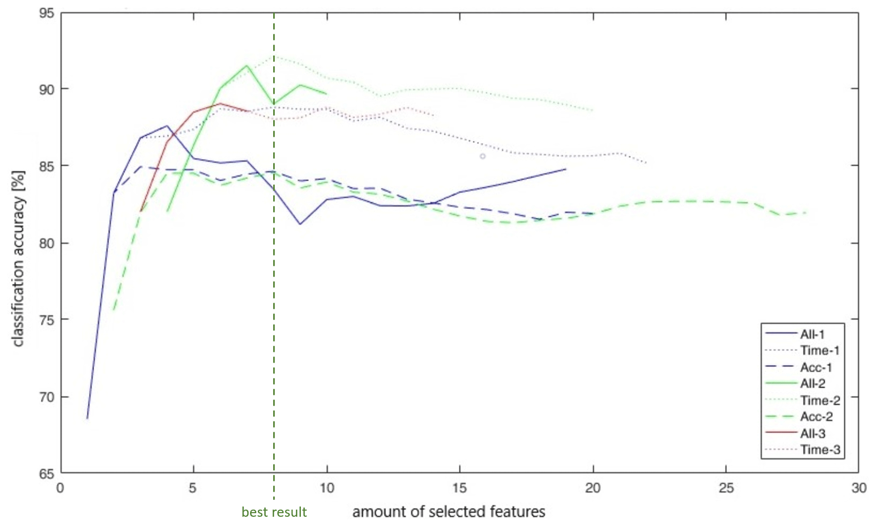
Figure 8Classification accuracies for different forward selection processes with offline data.
Figure 8 further tells us that if we only use features of the time domain, classification accuracy does not drop. If we only use data from the acceleration sensor, then the accuracy is somewhat lower.
For the forward selection process Acc-1 that uses only data of the acceleration sensor, Fig. 9a shows the corresponding classification accuracies for online data streams with the same selected features. The approach with offline data with three features achieved the highest classification accuracy (84.94 %), whereas with online data streams the best method (88.93 %) uses 12 features and a short time lag (see label Online-Lag1 in Fig. 9a). The label “Lag1” means that the last two classification estimates are used to formulate a new classification result. The option “Lag2” uses the last three estimates to formulate a new one. The maximum accuracy decides the class number. If two maxima are equal, the class with no key operation is preferred. Furthermore, all 12 subjects underwent a teaching process (offline data of all 12 subjects is used as training data).
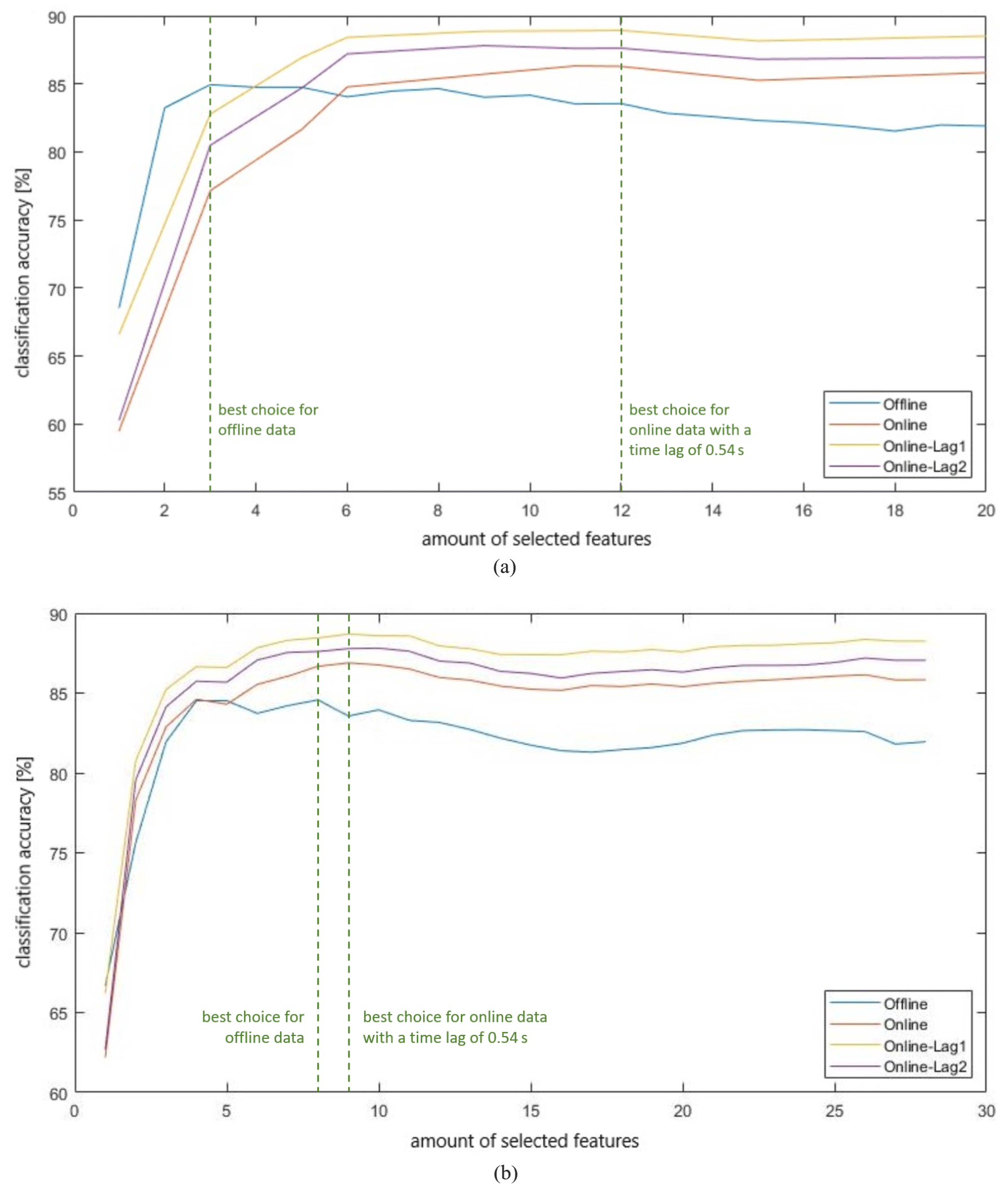
Figure 9Classification accuracies for two forward selection processes with offline and online data. (a) Forward selection process Acc-1; (b) forward selection process Acc-2.
Figure 9a tells us that with theoretical offline data fewer features can be used to get a good classification method, but in practice with online data streams more features are needed to get the same (or even a better) accuracy. For the forward selection process Acc-2 (with the two prescribed features 58+59 computed from acceleration data), the corresponding results for comparison of offline and online data are given in Fig. 9b. Here, the online approach is also with fewer features as good as the offline approach, but the highest classification accuracies attained are nearly the same as with process Acc-1 with 84.57 % for offline data and eight specific features and 88.69 % for online data and nine specific features.
6.1.5 Determination of a feature set
Based on the results depicted in Fig. 9b, we selected the nine specific features – found with use of online data streams and acceleration data only – as our choice for further examinations. This nine features are median, 75th percentile, skewness, kurtosis, harmonic mean, magnitudes of jerk, coefficient of variation and the preselected features energy in direction and in the orthogonal direction of gravity. Remarkably, this feature set does not contain features from the spectral domain. In our further analyses, we restrict our analysis to data of the acceleration sensor. In future work, this decision may be revised.
6.2 Further analyses with the specified classification method
In the following, seven different questions that came to mind have been studied.
6.2.1 Is a teaching process for each subject necessary?
To answer this question, the algorithm was trained with 1, 3, 5, 11 or all subjects and tested with the remaining subjects. In the case where all subjects served for training, all subjects also served for testing. Figure 10a illustrates the different classification accuracies for online data streams and different time lags (see also the paragraph of Fig. 9a for a description of these time lags).
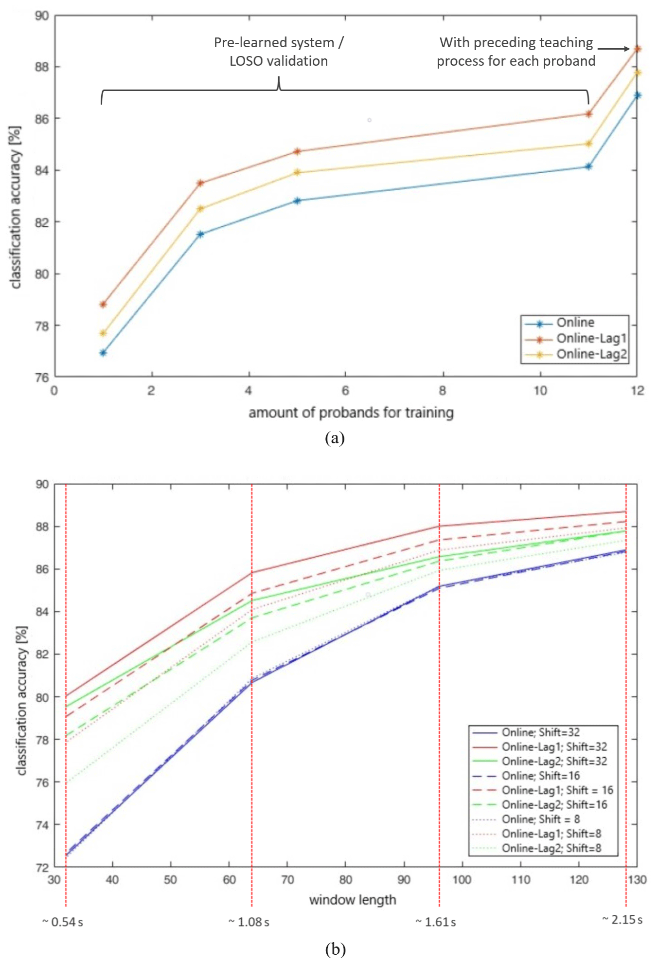
Figure 10Classification accuracies for different settings with online data. (a) Classification accuracies with and without a preceding teaching process; (b) classification accuracies for different window lengths and shifts.
The values depicted in Fig. 10a with 1 to 11 subjects for training behave like a pre-learnt system (no teaching for each subject necessary before using the therapy table), whereas with x axis = 12 we have a system with a going-ahead teaching process for each subject, but in the training database the data of the other subjects are also stored. The classification accuracy drops about 3 % for a system without teaching provided that many subjects pre-learnt the system (here 11 subjects). This figure underlines again the importance of the LOSO evaluation to simulate real-life settings.
We expect that the classification accuracy of a system without a foregoing teaching process saturates at about the value as depicted for 11 subjects, even if more subjects train the system, as the curve resembles processes with restricted growth.
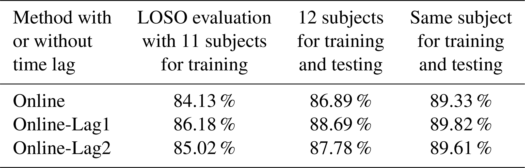
In the foregoing Sects. 4 and 5 with one skilled (and therefore rather precise) subject, we achieved classification accuracies of about 97 %. Considering the mean accuracies of all 12 subjects, where for training and testing only the data of one subject is used, we got 89.33 % for online data streams without a time lag (corresponds to label “Online”). Therefore, the best solution would be a training database with training data of only one person that also uses the system afterwards. In our studies, we saw widely varying classification accuracies, which we hypothesize to originate from the precision of how exercises, in particular the movements of the key exercises, are fulfilled. Classification accuracies therefore ranged from 76.33 % to 96.95 % for different subjects (label “Online”). So, the robustness of the system is only given if the key exercises are performed in a consistent and clear manner.
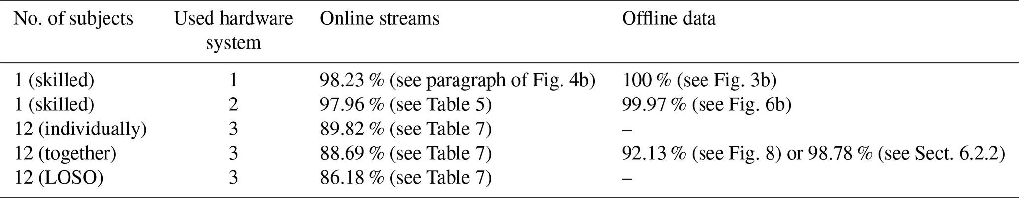
As this section is an essential result of our study, we summarize the most important accuracies in Table 7.
Table 7Classification accuracies for different evaluation techniques and 12 subjects with online data.
6.2.2 How many activities are distinguishable?
In the beginning of Sect. 6, we stated that five further possible movements for controlling the therapy table have been recorded for all 12 subjects. With seven key movements altogether (vertical pumping of a foot pump, horizontal pumping of a foot pump, stamping, toe-tipping, describing a circle with the knee, swinging the hips left and right, and quickly moving the knees forward and backward in an alternating manner) and the three activities go, run and massage, we may assess how good these 10 activities can be distinguished. Table 8 shows the classification accuracies when successively adding further activities. Therefore, we used all 118 features (we made no feature selection processes for each special number of activities to find the best subgroups, which may lead to an underestimation of the performances), recorded offline data and used a pre-learnt system with three subjects – in other words three subjects for training and nine different subjects for testing.
Table 8Classification accuracies for a different number of activities and a pre-learnt system with three subjects with offline data.
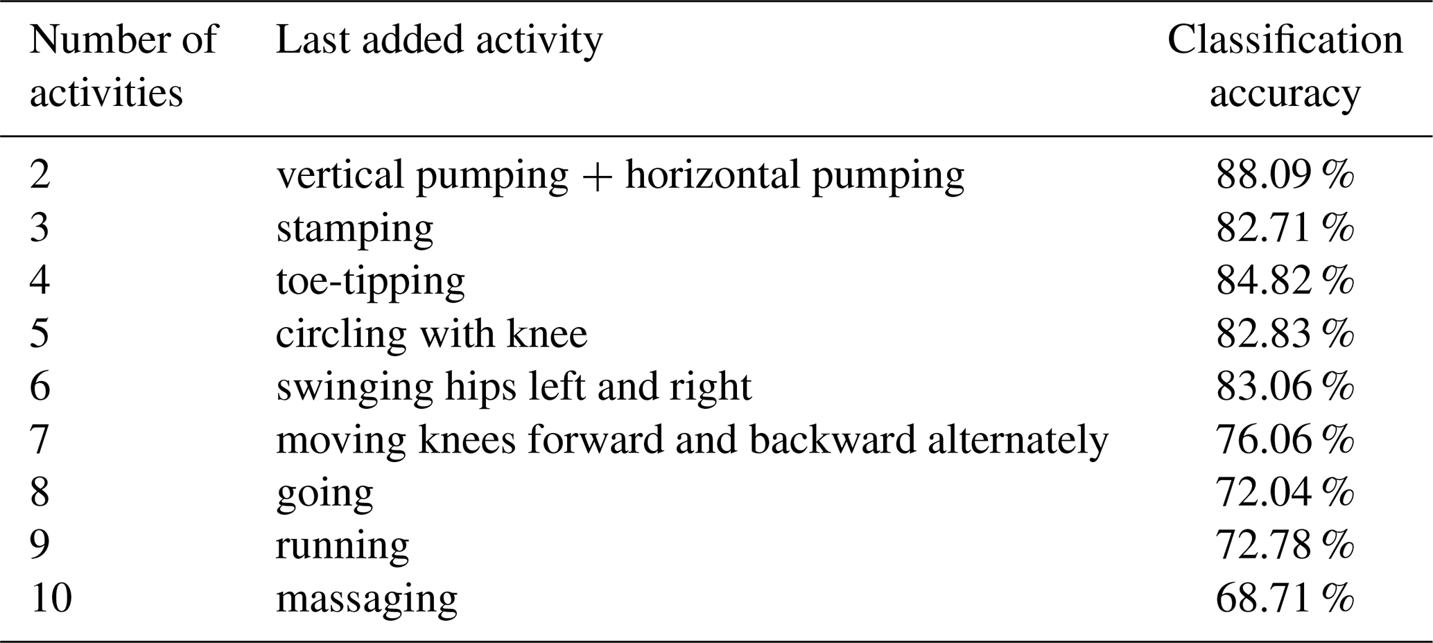
Please keep in mind that for a different order of adding these 10 activities, other accuracies also are achieved, but for all 10 activities, the classification accuracy remains the same. In conclusion, the classification accuracies in Table 8 are influenced by the feature set, the order of adding activities and the special character of a selected activity, as classification accuracies drop or increase after each addition. If we prefix a teaching process (all 12 subjects are pre-learnt in a database), the classification accuracies increase to 100 % for the first two activities and to 92.64 % for 10 activities. These facts highlight the importance of such a teaching process. If we choose the five activities vertical pumping, horizontal pumping, going, running and massaging for this evaluation, an accuracy of 98.78 % is achieved.
What if we use the best feature sets for offline data (eight specific features) and online data (nine specific features) found at the end of Sect. 6.1.4?
-
eight specific features: 91.93 % for 2 activities and 67.40 % for 10 activities,
-
nine specific features: 91.14 % for 2 activities and 55.11 % for 10 activities.
Due to these classification accuracies, we can see that these feature subsets have been optimized for the five activities of vertical and horizontal pumping, going, running, and massaging. To classify 10 classes, a new feature selection process would be necessary.
6.2.3 Analysis of different window lengths and shifts
For this analysis, online data streams, five classes as usual, a system with pre-learning through all 12 subjects and a good feature set found in Sect. 6.1.4 (nine specific features to classify five classes with online data) are used. Up to now, we set the window length to 128 and the window shift to 32. But now, we want to vary these parameters to see the changes in classification accuracy (see Fig. 10b).
For comparison of estimated and real states, the estimates are saved with the timestamp corresponding to the centre of the window (a procedure we used for all performance analyses). Therefore, the parameter window shift has no real influence on the performance of the system. As in the analysis before, the time lag announced as Lag1 gives the best results (the last two estimates are used to formulate a new one – see also Sect. 6.1.4 for more details about the used time lags). The best window length is still 128, but also a length of 96 would be feasible for our hardware system with a sample rate of 59.5 Hz. A window length of 64 or less is not recommendable here.
6.2.4 Is a minimal size of training database also good enough?
The aim of this study is to minimize the size of the training database. Here, we use five classes for classification (up to now we used three classes for the analysis with hardware system 3) and one averaged training data sample per activity group and per subject. After the computation of all means of the feature vectors, normalization to values between 0 and 1 is made. An example is shown in Fig. 11 for feature 11, which is the range of total acceleration.
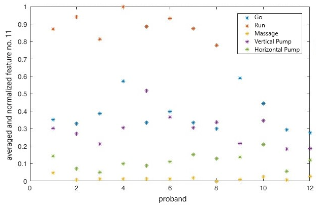
Figure 11Averaged and normalized feature no. 11 (range of total acceleration) for different subjects and activities with online data and a minimized training database.
The data points shown in Fig. 11 are stored in the training database for feature 11. In this figure, we also see that the range is similar for the activities going and vertical pumping (therapy table should drive up).
Further, the interesting question is now how does Fig. 8, which shows the classification accuracies for different forward feature selection processes with use for offline data, transform if we use this minimal database? The answer is contained in Fig. 12a, which shows the theoretical classification performances for seven forward feature selection processes with different feature sets.
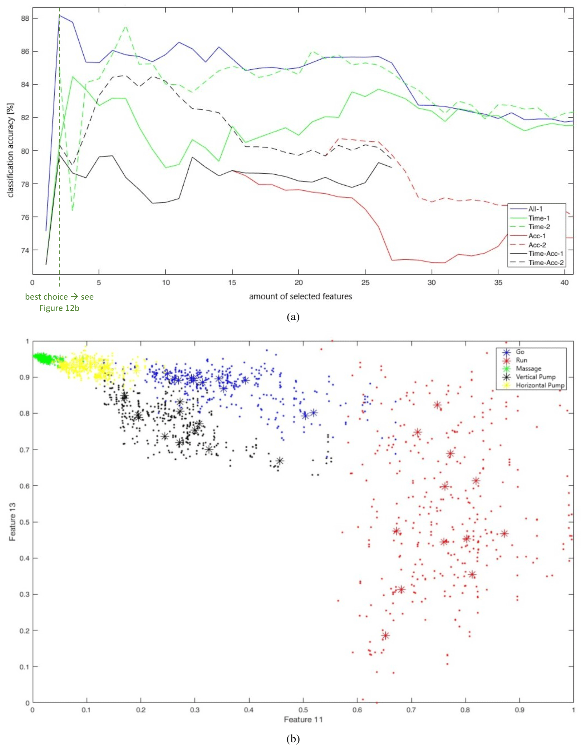
Figure 12Usage of a minimized training database. (a) Classification accuracies for different forward selection processes with offline data; (b) comparison of test and training data samples for feature 11+13 (best combination of two features with offline data).
In the labelling, “−1” stands for no preselected features and “−2” for a preselection of features 58+59 of acceleration data. “All” means again that the process starts with all features, and “Time”, “Acc”, or “Time-Acc” mean that only features from the time domain, from the acceleration sensor, or from time the domain and acceleration sensor are used. As one might expect, the classification accuracies drop in comparison to the results depicted in Fig. 8; however, the classification accuracies of the single features did not decline. The classification accuracies also drop slightly with use of online data streams.
One big advantage of this minimal training database is that a grid search is feasible to find the best global feature selection set due to much less comparisons with training data samples. If we consider the 28 features of the group Time-Acc-1 (feature numbers 1–26 and 58–59 of Sect. 6.1.1), the best and worst feature combinations of the grid search are given in Table 9.
Table 9Classification accuracies of grid search for a different size of the feature set with offline data.
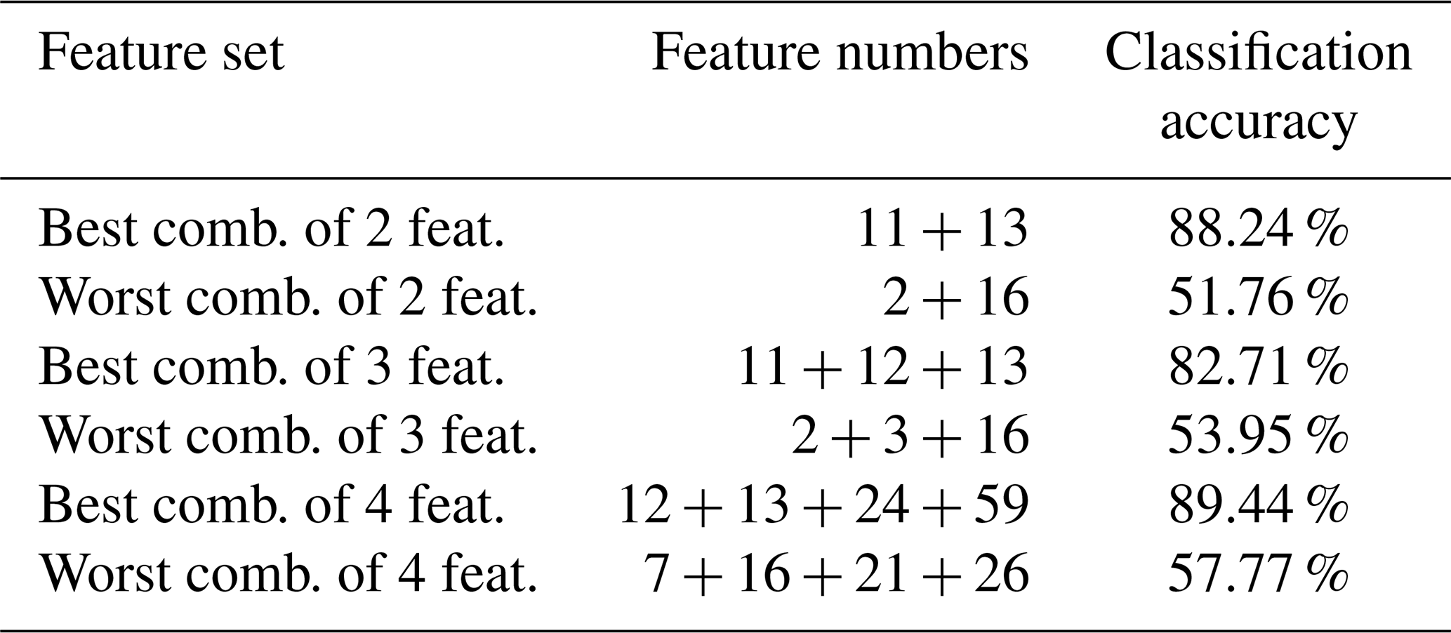
Table 9 shows that the classification accuracies resulting from a grid search are much higher than by a forward feature selection process. In Fig. 12a with features selected from the set Time-Acc-1, for instance, we achieved accuracies between 78 % and 80 % for a feature set consisting of 2 to 4 features, now we achieved accuracies between 82 % and 90 %. So, theoretically, it makes sense to use the grid search if it is somehow possible.
Figure 12b exemplary shows the test and training data samples that have to be compared for the best combination with a feature set size of 2. The asterisks mark the training data and the points mark the test data.
With these three possible feature pre-selections found by grid search, new forward feature selection processes were initiated. For offline data, a better method for five features was found (feature numbers 12 + 13 + 24 + 59 + 15) with an accuracy of 89.85 % but no more remarkable improvements. Unfortunately, the optimal feature sets found with offline data could not transfer their good performance to online data streams. Here, the feature set announced in Sect. 6.1.5 is still the best method, i.e. 85.40 % without time lag and 87.52 % with Lag1.
This approach may be a feasible alternative if many subjects train the system. If only one person trains the system, only five means are saved in the training database, and this is somehow too low. Here, it would be better to save not only one but several means per activity. Subject 1, for instance, had an accuracy of 97 % with a foregoing teaching process, but with a minimal database accuracy dropped to 94 %, which would not be a good idea.
6.2.5 Is a parameter k larger than 1 better suited?
In the course of the analysis, evaluations with k = 3 and k = 5 have been made. As results changed only slightly (sometimes for the better, sometimes for the worse) k = 1 is still a good choice.
6.2.6 Are support vector machines (SVMs) a superior alternative?
For the implementation of support vector machines in MATLAB, the free library LIBSVM has been used. In the function options of svmtrain(), many parameters can be set – for our analyses we mainly focused at the SVM-type C-SVM with radial basis function kernel. For the training database, we did not use the minimal database as SVMs need a lot of data for training. We used balanced training datasets with five possible activities. In Table 10, the best results are summarized.
Table 10Classification accuracies for SVMs with different feature sets and parameters with online data.
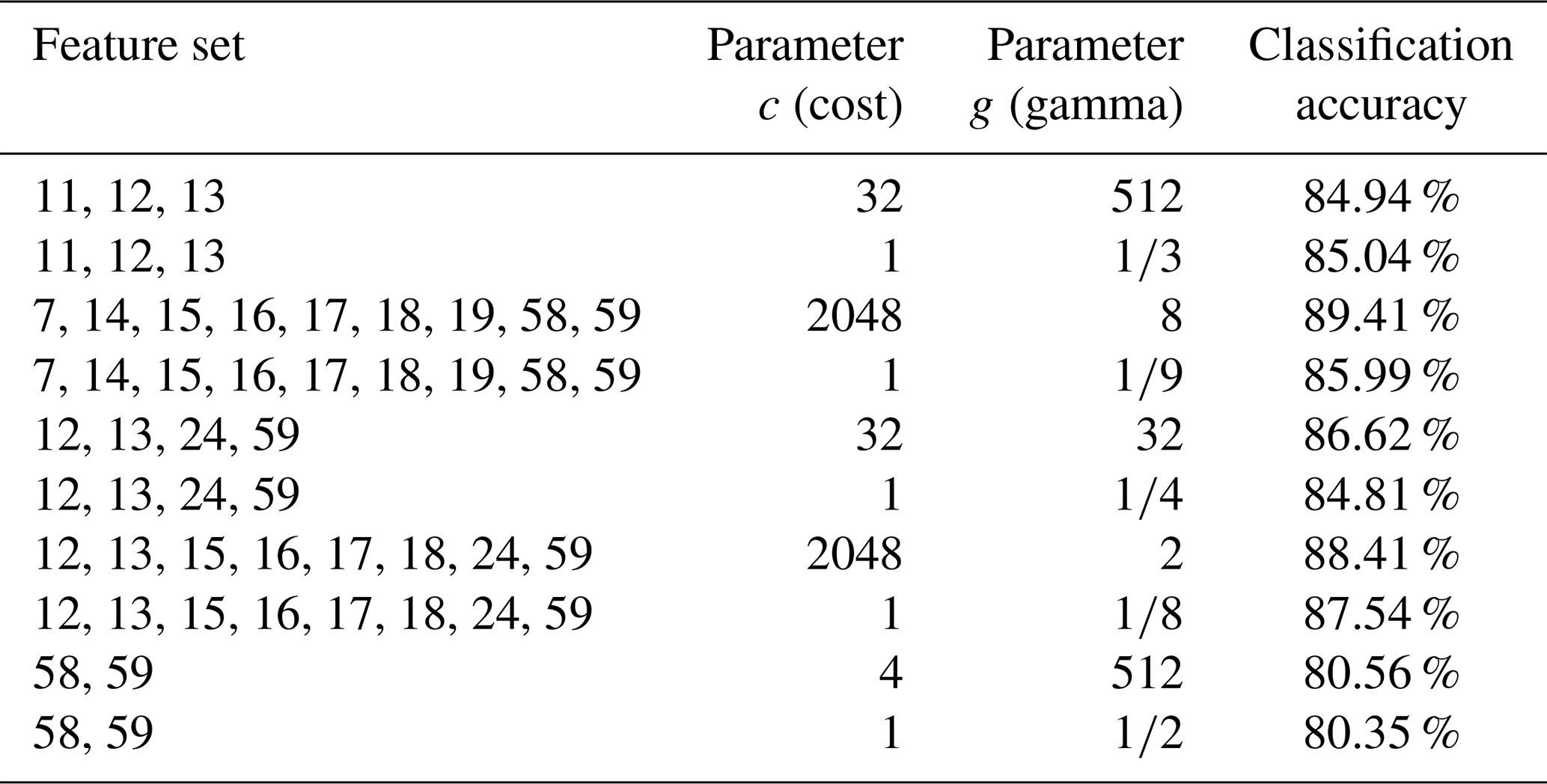
Here, we used the online data approach with good feature sets found by the KNN method for features of the time domain and acceleration sensor. Details for the used features can be found in Sect. 6.1.1. For the parameters c (cost) and g (gamma), on the one hand, we used default values (c=1 and ), and on the other hand, we used values found by cross-validation combined with a grid search. Here, the features fixed in Sect. 6.1.5 are again the best choice with use of online data streams (89.41 %) – this is a little bit better than with use of the 1NN method (87.73 %). Please keep in mind that the training phase of SVMs is more time-consuming as suitable parameters for a special feature set have to be found to be as good as KNN methods. If we make a teaching process with one subject to get training data and afterwards we test the system with the same subject, we get nearly the same mean performance (89.72 % instead of 89.41 %). For KNN methods, the performance could be increased with this aspect, but for SVM probably not. For this analysis, we used the best feature set with nine features of Table 10 (see row 3) with online data streams and 12 subjects. One subject, who performed the exercises more precisely, gained 96.71 %. So, we can see that it is important to make the key exercises precisely to also get a good system.
6.2.7 Is a hybrid method (SVM+1NN) the better choice?
In our study, we also researched whether combinations of support vector machines with 1NN methods provide a better classification result. We tested three different possibilities:
- 1.
The 1NN method with nine features fixed in Sect. 6.1.5 plus the SVM method with nine features announced in row 3 in Table 10.
- 2.
The 1NN method with nine features fixed in Sect. 6.1.5 plus the SVM method with nine features announced in row 3 in Table 10 plus the SVM method with four features announced in row 5 in Table 10.
- 3.
The 1NN method with nine features fixed in Sect. 6.1.5 plus the SVM method with nine features announced in row 3 in Table 10 plus the SVM method with eight features announced in row 7 in Table 10.
Attempt 1 combines the 1NN method with an SVM by making a motor control if both methods classified the same key exercise and by making no motor control if both methods are divided. Attempts 2 and 3 trigger a motor control if at least two methods plead for the same key exercise. The reached classification accuracies for these three attempts with use of online data streams are 88.71 %, 78.60 % and 88.92 %. So, this access to the hybrid methods did not lead to a performance improvement.
In Table 11, the details for the best-reached classification accuracies of Sects. 4–6 are summarized.
Table 11Best-reached classification accuracies for different settings.
The reasons for very good classification accuracies with one subject can be summarized as follows:
- 1.
The person is skilled, so the algorithm behind the system is known and, therefore, clear and consistent motions are beneficial.
- 2.
The trouser pockets are very deep, and this results in more information that can be captured from the distinct motions. The further the sensor is located from the hip or belt position towards a body part with a wide range of motion, the more information can be collected. This is also stated in Kulchyk and Etemad (2019).
- 3.
In the training database only data of one subject is stored. So, the speeds of performing a motion, such as running, are less varied.
Especially for analyses with the LOSO validation, it is known that classification accuracies are lower as with cross-validation. For instance, in Kulchyk and Etemad (2019) and Altun et al. (2010), the LOSO validation reached an accuracy of 78.35 % and 87.6 %, respectively. Our result of 86.18 % is similarly good, but please keep in mind that we computed this result out of our online data streams. For comparison purposes of our classification accuracies to others, we would like to emphasize that the accuracies in literature typically correspond to our offline data approach, where signal segments are extracted very carefully from different classes.
In this study, a HAR system carried by masseurs for controlling a therapy table via different movements of a single leg has been developed. In our experiments, we studied two different sensor positions: fixed at the right hip like a belt and loosely inserted in one pocket of the trousers. The second position turned out best, as movements are more distinct.
With one female subject, classification accuracies of about 98 % for online data streams (following a predefined protocol of movements) and up to 100 % for offline data samples (precise extraction of signal samples of distinct classes) were achieved. Thereby, three operating classes have been used: pump the therapy table up (class 2), pump the therapy table down (class 3) and do nothing (class 1) for all other activities performed by the masseur.
Furthermore, we conducted studies with 12 subjects and many different approaches and modifications. In conclusion, the classification accuracies varied in the range of 84 % to 98 % with, for instance, different validation techniques. In contrast to other literature studies, our results are comparably good.
With several subjects, the use of a minimal training database and/or a foregoing teaching process that may result in similar data for the training database may be worth consideration.
For future work, we additionally focus on key activities with a high frequency (double-clicks or tapping motions) such that the reaction time of the system can be further reduced, as the motor control cannot be faster as 1–2 cycle durations of these key motions. Moreover, we will study a special two-stage system to allow for remote control only if a special key is activated (for instance by an additional sensor or voice control).
The underlying data and coding are not publicly available.
ES led the project and made the concept and funding acquisition. ES and KlP developed the hardware. KlP prepared the data curation process, which was fulfilled by SaS. SaS developed the model code and performed the simulations. SaS prepared the manuscript with contributions and proofreading from all co-authors.
The contact author has declared that none of the authors has any competing interests.
Publisher’s note: Copernicus Publications remains neutral with regard to jurisdictional claims made in the text, published maps, institutional affiliations, or any other geographical representation in this paper. While Copernicus Publications makes every effort to include appropriate place names, the final responsibility lies with the authors.
This work has been supported by the COMET-K2 centre of the Linz Center of Mechatronics (LCM), funded by the Austrian federal government and the federal state of Upper Austria.
This research has been supported by the Österreichische Forschungsförderungsgesellschaft (grant no. 886468). This work has also been supported by the COMET-K2 centre of the Linz Center of Mechatronics (LCM), funded by the Austrian federal government and the federal state of Upper Austria.
This paper was edited by Robert Kirchner and reviewed by three anonymous referees.
Abdullah, C. S., Kawser, M., Islam Opu, M. T., Faruk, T., and Islam, M. K.: Human Fall Detection using built-in smartphone accelerometer, in: 2020 IEEE International Women in Engineering (WIE) Conference on Electrical and Computer Engineering (WIECON-ECE), Bhubaneswar, India, 26–27 December 2020, IEEE, 372–375, https://doi.org/10.1109/WIECON-ECE52138.2020.9398010, 2020. a, b, c, d
Altun, K., Barshan, B., and Tunçel, O.: Comparative study on classifying human activities with miniature inertial and magnetic sensors, Pattern Recogn., 43, 3605–3620, https://doi.org/10.1016/j.patcog.2010.04.019, 2010. a, b, c, d, e, f, g, h
Antoni, J. and Randall, R. B.: The spectral kurtosis: application to the vibratory surveillance and diagnostics of rotating machines, Mech. Syst. Signal Pr., 20, 308–331, https://doi.org/10.1016/j.ymssp.2004.09.002, 2006. a
Ashwini, K., Amutha, R., Rajave, R., and Anusha, D.: Classification of daily human activities using wearable inertial sensor, in: 2020 International Conference on Wireless Communications Signal Processing and Networking (WiSPNET), Chennai, India, 4–6 August 2020, IEEE, 1-6, https://doi.org/10.1109/WiSPNET48689.2020.9198406, 2020. a, b, c, d, e, f
Bajric, R., Zuber, N., Skrimpas, G. A., and Mijatovic, N.: Feature Extraction Using Discrete Wavelet Transform for Gear Fault Diagnosis of Wind Turbine Gearbox, Shock Vib., 2016, 6748469, https://doi.org/10.1155/2016/6748469, 2016. a
Beritelli, F., Casale, S., Russo, A., and Serrano, S.: A Genetic Algorithm Feature Selection Approach to Robust Classification between “Positive” and “Negative” Emotional States in Speakers, in: Conference Record of the Thirty-Ninth Asilomar Conference on Signals, Systems and Computers, Pacific Grove, CA, USA, 30 October–2 November 2005, IEEE, 550–553, https://doi.org/10.1109/ACSSC.2005.1599809, 2005. a
Bloomfield, R. A., Teeter, M. G., and McIsaac, K. A.: Convolutional Neural Network approach to classifying activities using knee instrumented wearable sensors, IEEE Sens. J., 20, 14975–14983, https://doi.org/10.1109/JSEN.2020.3011417, 2020. a, b, c, d, e, f
Büber, E. and Guvensan, A. M.: Discriminative time-domain features for activity recognition on a mobile phone, in: 2014 IEEE Ninth International Conference on Intelligent Sensors, Sensor Networks and Information Processing (ISSNIP), Singapore, 21–24 April 2014, IEEE, 1–6, https://doi.org/10.1109/ISSNIP.2014.6827651, 2014. a, b, c, d, e, f, g
Capela, N. A., Lemaire, E. D., and Baddour, N.: Feature Selection for Wearable Smartphone-Based Human Activity Recognition with Able bodied, Elderly, and Stroke Patients, PLoS ONE, 10, e0124414, https://doi.org/10.1371/journal.pone.0124414, 2015. a
Chang, C.-C. and Lin, C.-J.: LIBSVM: A Library for Support Vector Machines, Association for Computing Machinery, 2, 1–27, https://doi.org/10.1145/1961189.1961199, 2011. a
Chuang, F.-C., Wang, J.-S., Yang, Y.-T., and Kao, T.-P.: A wearable activity sensor system and its physical activity classification scheme, in: The 2012 International Joint Conference on Neural Networks (IJCNN), Brisbane, QLD, Australia, 10–15 June 2012, IEEE, 1–6, https://doi.org/10.1109/IJCNN.2012.6252581, 2012. a, b, c, d
Fernandes, V., Mascarehnas, L., Mendonca, C., Johnson, A., and Mishra, R.: Speech Emotion Recognition using Mel Frequency Cepstral Coefficient and SVM Classifier, in: 2018 International Conference on System Modeling & Advancement in Research Trends (SMART), Moradabad, India, 23–24 November 2018, IEEE, 200–204, https://doi.org/10.1109/SYSMART.2018.8746939, 2018. a
Gupta, P. and Wadhwani, S.: Feature selection by genetic programming, and artificial neural network-based machine condition monitoring, International Journal of Engineering and Innovative Technology (IJEIT), 1, 177–181, 2012. a
Kim, H.-d., Park, C.-h., Yang, H.-c., and Sim, K.-b.: Genetic Algorithm Based Feature Selection Method Development for Pattern Recognition, in: 2006 SICE-ICASE International Joint Conference, Busan, Korea (South), 18–21 October 2006, IEEE, 1020–1025, https://doi.org/10.1109/SICE.2006.315742, 2006. a, b
Kulchyk, J. and Etemad, A.: Activity recognition with wearable accelerometers using Deep Convolutional Neural Network and the effect of sensor placement, 2019 IEEE SENSORS, Montreal, QC, Canada, 27–30 October 2019, IEEE, 1–4, https://doi.org/10.1109/SENSORS43011.2019.8956668, 2019. a, b, c, d, e, f, g, h
Mannini, A. and Sabatini, A. M.: On-line classification of human activity and estimation of walk-run speed from acceleration data using support vector machines, in: 2011 Annual International Conference of the IEEE Engineering in Medicine and Biology Society, Boston, MA, USA, 30 August–3 September 2011, IEEE, 3302–3305, https://doi.org/10.1109/IEMBS.2011.6090896, 2011. a, b, c
Meyer-Baese, A. and Schmid, V.: Chapter 2 – Feature Selection and Extraction, in: Pattern Recognition and Signal Analysis in Medical Imaging, 2nd edn., Academic Press, 21–69, https://doi.org/10.1016/B978-0-12-409545-8.00002-9, 2018. a, b
Morris, D., Saponas, T. S., Guillory, A., and Kelner, I.: RecoFit: using a wearable sensor to find, recognize, and count repetitive exercises, in: CHI '14: CHI Conference on Human Factors in Computing Systems Toronto Ontario, Canada, 26 April–1 May 2014, Association for Computing Machinery, 3225–3234, https://doi.org/10.1145/2556288.2557116, 2014. a
Nandi, A. K., Liu, Ch., and Wong, M. L. D.: Intelligent Vibration Signal Processing for Condition Monitoring, in: 2013 International Conference Surveillance 7, 29–30 October 2013, Chartres, France, https://surveillance7.sciencesconf.org/conference/surveillance7/P1_Intelligent_Vibration_Signal_Processing_for_Condition_Monitoring_FT.pdf (last access: 5 July 2024), 2013. a
Nguyen, P., Akiyama, T., Ohashi, H., Nakahara, G., Yamasaki, K., and Hikaru, S.: User-friendly activity recognition using SVM classifier and informative features, in: 2015 International Conference on Indoor Positioning and Indoor Navigation (IPIN), Banff, AB, Canada, 3–16 October 2015, IEEE, 1–8, https://doi.org/10.1109/IPIN.2015.7346783, 2015. a, b, c, d, e, f, g
Pichler, K., Ooijevaar, T., Hesch, C., Kastl, C., and Hammer, F.: Data-driven vibration-based bearing fault diagnosis using non-steady-state training data, J. Sens. Sens. Syst., 9, 143–155, https://doi.org/10.5194/jsss-9-143-2020, 2020. a
Preece, S. J., Goulermas, J. Y., Kenney, L. P. J., and Howard, D.: A comparison of feature extraction methods for the classification of dynamic activities from accelerometer data, IEEE T. Bio-Med. Eng., 56, 871–879, https://doi.org/10.1109/TBME.2008.2006190, 2009. a
Prieto, M. D., Cirrincione, G., Espinosa, A. G., Ortega, J. A., and Henao, H.: Bearing fault detection by a novel condition-monitoring scheme based on statistical-time features and neural networks, IEEE T. Ind. Electron., 60, 3398–3407, https://doi.org/10.1109/TIE.2012.2219838, 2012. a
Rabiner, L. R.: A tutorial on hidden Markov models and selected applications in speech recognition, P. IEEE, 77, 257–286, https://doi.org/10.1109/5.18626, 1989. a
Rosso, O. A., Blanco, S., Yordanova, J., Kolev, V., Figliola, A., Schürmann, M., and Başar, E.: Wavelet entropy: a new tool for analysis of short duration brain electrical signals, J. Neurosci. Meth., 105, 65–75, https://doi.org/10.1016/s0165-0270(00)00356-3, 2001. a
Saha, J., Chakraborty, S., Chowdhury, C., Biswas, S., and Aslam, N.: Designing device independent two-phase activity recognition framework for smartphones, in: 2017 IEEE 13th International Conference on Wireless and Mobile Computing, Networking and Communications (WiMob), Rome, Italy, 9–11 October 2017, IEEE, 257–264, https://doi.org/10.1109/WiMOB.2017.8115841, 2017. a, b, c, d, e, f, g, h
San Buenaventura, C. V. and Tiglao, N. M. C.: Basic human activity recognition based on sensor fusion in smartphones, in: 2017 IFIP/IEEE Symposium on Integrated Network and Service Management (IM), Lisbon, Portugal, 8–12 May 2017, IEEE, 1182–1185, https://doi.org/10.23919/INM.2017.7987459, 2017. a, b, c, d, e, f
Shen, Ch., Wang, D., Kong, F., and Tse, P. W.: Fault diagnosis of rotating machinery based on the statistical parameters of wavelet packet paving and a generic support vector regressive classifier, Measurement, 46, 1551–1564, https://doi.org/10.1016/j.measurement.2012.12.011, 2013. a
Singh, S. and Vishwakarma, M. K.: A Review of Vibration Analysis Techniques for Rotating Machines, International Journal of Engineering Research & Technology (IJERT), 4, 757–761, https://www.ijert.org/a-review-of-vibration-analysis-techniques-for-rotating-machines (last access: 5 July 2024), 2015. a
Ustev, Y. E., Incel, O. D., and Ersoy, C.: User, device and orientation independent human activity recognition on mobile phones: Challenges and a proposal, in: Proceedings of the 2013 ACM Conference on Pervasive and Ubiquitous Computing Adjunct Publication – UbiComp '13 Adjunct, Zurich, Switzerland, 8–12 September 2013, Association for Computing Machinery, 1427–1436, https://doi.org/10.1145/2494091.2496039, 2013. a, b, c, d, e, f
Weng, S., Xiang, L., Tang, W., Yang, H., Zheng, L., Lu, H., and Zheng, H.: A low power and high accuracy MEMS sensor based activity recognition algorithm, in: 2014 IEEE International Conference on Bioinformatics and Biomedicine (BIBM), Belfast, UK, 2–5 November 2014, IEEE, 33–38, https://doi.org/10.1109/BIBM.2014.6999238, 2014. a, b, c, d, e
Yang, F. and Zhang, L.: Real-time human activity classification by accelerometer embedded wearable devices, in: 2017 4th International Conference on Systems and Informatics (ICSAI), Hangzhou, China, 11–13 November 2017, IEEE, 469–473, https://doi.org/10.1109/ICSAI.2017.8248338, 2017. a, b, c
Yi, S., Mirowski, P., Ho, T. K., and Pavlovic, V.: Pose Invariant Activity Classification for Multi-floor Indoor Localization, in: 2014 22nd International Conference on Pattern Recognition, Stockholm, Sweden, 24–28 August 2014, IEEE, 3505–3510, https://doi.org/10.1109/ICPR.2014.603, 2014. a
Zhang, X. H., Kang, J. S., Zhao, J., and Duanchao, C.: Features for Fault Diagnosis and Prognosis of Gearbox, Chem. Engineer. Trans., 33, 1027–1032, https://doi.org/10.3303/CET1333172, 2013. a
- Abstract
- Introduction
- Related work
- Hardware and software infrastructure
- Experimental results and discussion for hardware system 1
- Experimental results and discussion for hardware system 2
- Experimental results and discussion for hardware system 3
- Comparison of classification accuracies for hardware systems 1–3
- Conclusions and future work
- Code and data availability
- Author contributions
- Competing interests
- Disclaimer
- Acknowledgements
- Financial support
- Review statement
- References