The River Runner: a low-cost sensor prototype for continuous dissolved greenhouse gas measurements

Freshwater ecosystems are sources of the two most relevant greenhouse gases (GHGs): CO₂ and CH₄. Understanding the importance of freshwater ecosystems in the global carbon cycle and their role in global warming trends requires the accurate quantification of gas fluxes from the water phase to the atmosphere. These fluxes depend on the gas exchange velocity and the concentration gradient between the phases, which both cause high spatio-temporal variability in fluxes. On a global scale, the estimation of fluxes is limited by the lack of cheap and accurate methods to measure dissolved gas concentrations. Low-cost sensors, as an alternative to expensive gas analysers, are available; however, to date, the in situ performance of such sensors has been poorly examined. Here, we present an inexpensive data-logging sensor prototype that provides continuous measurements of dissolved CO₂ and CH₄ in submerged environments. Gas measurements are done in a confined gas space, which is rapidly equilibrated with the water phase through a single-layer polytetrafluoroethylene (PTFE) membrane, by a miniature non-dispersive infrared (NDIR) sensor for CO₂ (Sunrise sensor, Senseair, Sweden) and a cheap metal oxide sensor for CH₄ (TGS2611-E, Figaro Engineering Inc., Japan). Pressure, temperature and humidity are measured to correct raw sensor readings. For freshwater, the dissolved gas concentration is directly obtained from the measured molar fraction and temperature and pressure readings. In air, we measured the molar fraction of CO₂ in a range from 400 to 10 000 ppm and the molar fraction of CH₄ in a range from 2 to 50 ppm with an accuracy of ± 58 and ± 3 ppm respectively. We successfully used our prototype to measure diurnal variations in dissolved CO₂ in a natural stream. We further calibrated the CH₄ sensor for in situ use at concentrations ranging from 0.01 to 0.3 µmol L⁻¹. Underwater, we were able to measure the molar fraction of CH₄ in the prototype head with an accuracy of ± 13 ppm in the range from 2 to 172 ppm. The underwater measurement error of CH₄ is always higher than for the same concentration range in air, and CH₄ is highly overestimated below 10 ppm. At low CH₄, humidity was the most important influence on the TGS2611-E sensor output in air, whereas temperature became the predominant factor underwater. We describe the response behaviour of low-cost sensors in submerged environments and report calibration methods to correct for temperature and humidity influence on the sensor signal if used underwater. Furthermore, we provide do-it-yourself instructions to build a sensor for submerged continuous measurements of dissolved CO₂ and CH₄. Our prototype does not rely on an external power source, and we anticipate that such robust low-cost sensors will be useful for future studies of GHG emissions from freshwater environments.

1 Introduction

Freshwater ecosystems receive, transform, store and transport significant quantities of terrestrial carbon (Cole et al., 2007). In total, global inland waters receive approximately 5.1 Pg C yr⁻¹ from adjacent terrestrial ecosystems, of which estimated amounts of 0.9 and 0.6 Pg C yr⁻¹ are exported to oceans and stored in sediments respectively (Drake et al., 2018). Over the last decade, the historically underestimated outgassing flux has been repeatedly refined due to new data; estimates have ranged from 0.75 (Cole et al., 2007) to 3.9 Pg C yr⁻¹ (Drake et al., 2018). Most of these gaseous carbon flux estimates pertain to CO₂, yet outgassing of carbon from freshwater ecosystems occurs in the form of methane (CH₄) and carbon dioxide (CO₂) (Cole et al., 2007; Bastviken et al., 2011; Rosentreter et al., 2021). These two gases are among the most important greenhouse gases (GHGs) contributing to global warming (Saunois et al., 2019).

Substantial uncertainties in the estimation of global GHG fluxes to the atmosphere are caused by the high variability in ecosystem-scale fluxes in space and time. This is especially true for small streams and rivers, which are under-represented in the scientific literature, even though they have the highest and most variable gas exchange velocities (Raymond et al., 2013), the highest partial pressures of GHGs (Butman and Raymond, 2011), and the most difficult to estimate global surface area (Raymond et al., 2013). Direct flux measurements, for example, using drifting flux chambers (Lorke et al., 2015) or eddy covariance technology (Huotari et al., 2013), are largely impractical in small lotic ecosystems due to the physical challenges of flowing water and the spatial extent and shape of streams and rivers. Thus, fluxes are usually estimated as the product of a concentration gradient to the atmosphere and the gas exchange velocity. Whereas the latter can be predicted from physical features (Raymond et al., 2012), the highly variable concentration is ideally estimated over relevant diurnal and seasonal timescales as well as across many systems. Here, a major bottleneck to estimate GHG emissions from these systems is the lack of cheap and sufficiently accurate measurement methods for dissolved CO₂ and CH₄ (Drake et al., 2018; Bastviken et al., 2020).

Current methods to measure GHG concentrations mostly rely on expensive equipment or include labour-intensive procedures and analyses. To date, the dissolved gas concentration is mostly analysed using the headspace technique, equilibrators or semipermeable membranes. The headspace method includes collecting discrete water samples followed by a gas extraction step (equilibration with small gaseous headspace) and consequent gas analysis (Boulart et al., 2010). Realistically, this method allows only either high spatial or temporal coverage, as it is time-demanding and costly due to sample analysis by gas chromatography or with a closed loop on a portable gas analyser (Wilkinson et al., 2018).

More efficient data collection may be possible with in situ measurements of dissolved gases, for example, involving the use of an equilibrator in a loop with a portable gas analyser. Here, the gas–liquid exchange area is increased by a membrane, marbles or the formation of water droplets (e.g. spray type equilibrator) (Yoon et al., 2016). Subsequent analysis by a portable trace gas analyser allows real-time measurements (Boulart et al., 2010; Paranaíba et al., 2018; Xiao et al., 2020; Dalvai Ragnoli et al., 2023). Nevertheless, the analysis of GHG spatial variability is limited by the number of (mostly expensive) analysers.

A cheaper approach to measure greenhouse gases, at least for CO₂, is by non-dispersive infrared (NDIR) sensors, which – when combined with semipermeable membranes – allow for the submergence of gas sensors as well as continuous in situ measurements (Johnson et al., 2006, 2010; Leith et al., 2015). Concentration is measured in the gaseous headspace enclosed behind the membrane, which is assumed to be in equilibrium with the water phase. Using measurement intervals of between 5 and 10 min, such devices have recorded diurnal fluctuations in a peatland stream (Dinsmore and Billett, 2008) and storm-induced pulses of high CO₂ concentrations in a forested headwater in an Amazonian stream (Johnson et al., 2006, 2007). In these cases, measurements compared well with discrete headspace measurements done in parallel with a gas chromatograph (Dinsmore et al., 2009; Johnson et al., 2007).

In recent years, there has been a rise in self-made microprocessor-based logger configurations equipped with relatively cheap sensors to monitor air quality and atmospheric GHG concentrations (van den Bossche et al., 2017; Collier-Oxandale et al., 2018; Jørgensen et al., 2020), emissions from aquatic environments by flux chambers (Duc et al., 2013; Bastviken et al., 2015, 2020), or bubble emissions (Thanh Duc et al., 2019; Maher et al., 2019).

A sensor type showing promising results with respect to monitoring the CH₄ concentration, even at atmospheric levels, is the Taguchi gas sensor (TGS) family from Figaro Engineering Inc. (Osaka, Japan) (Eugster and Kling, 2012; van den Bossche et al., 2017; Collier-Oxandale et al., 2018; Eugster et al., 2020; Bastviken et al., 2020; Jørgensen et al., 2020). The TGS2600 sensor model has been successfully used for preliminary studies in the search for potential methane hot spots (Eugster and Kling, 2012) and to examine air quality trends at small spatial and temporal scales (Collier-Oxandale et al., 2018), whereas the TGS2611-E sensor model has been successfully used to measure CH₄ concentrations down to the level of near-ambient concentrations (van den Bossche et al., 2017; Jørgensen et al., 2020; Bastviken et al., 2020).

Here, we describe and provide the blueprint to replicate our River Runner (RR) prototype: a self-built, low-cost, submersible logger equipped with cheap gas sensors to measure dissolved CH₄ and CO₂ continuously and in situ. The gas sensors are covered by a gas-permeable membrane that separates the sensor area, with a confined gas space, from the water phase and allows for equilibration between both phases. The CH₄ sensor of our choice is the TGS2611-E. This sensor acts as a variable voltage divider, and resistance varies with the presence of CH₄, humidity and temperature. Therefore, a two-step calibration is necessary; here, we report an easy-to-use calibration method for submerged measurements. Concurrently, CO₂ is measured with a new cheap NDIR-based sensor that is factory-calibrated and ready to use. The blueprint of our prototype and calibration instructions for in situ measurements allow one to easily replicate our prototype. We anticipate that our device will help to address uncertainties in GHG flux emissions by providing robust measurements from highly variable and remote aquatic systems like small streams and rivers. The sensor accuracy of the cheap gas sensors is compensated for by the low investment costs, which allow one to install a larger set of replicated sensors to simultaneously address the temporal variability and spatial heterogeneity of the surveyed systems.

2 Material and methods

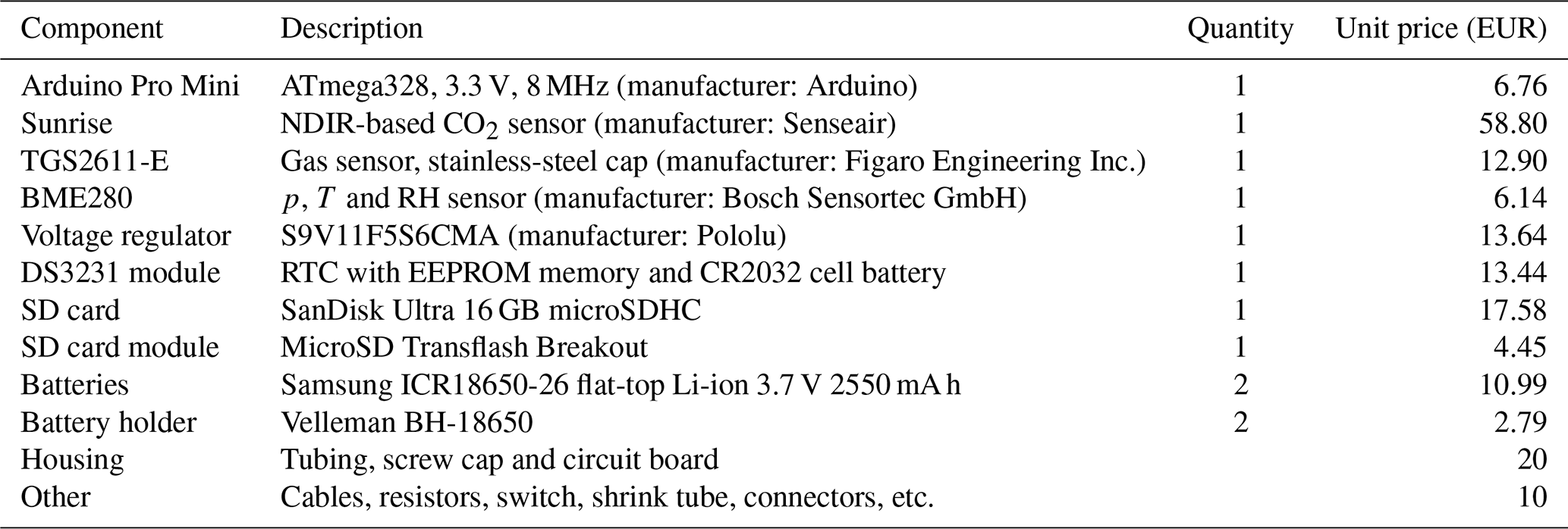
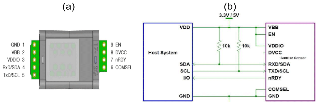
The River Runner prototype is built to measure dissolved CH₄ and CO₂ continuously and in situ. Hardware and electronics are embedded in a polypropylene-based tubing designed for water pipes in kitchen sinks. The prototype is divided into two parts, namely, the prototype body and the prototype head (Fig. 1). While the prototype body houses electrical hardware and batteries and is, thus, placed inside the tubing to be completely waterproof, the prototype head holds the gas sensors, which are placed outside of the prototype body and separated from the water phase by a semipermeable membrane. The polytetrafluoroethylene (PTFE) membrane used is hydrophobic, but its permeability to gases allows for the gaseous phase in the prototype head to equilibrate with the water phase. The membrane was chosen due to a good compromise between gas diffusivity, liquid entry pressure and mechanical strength (a description and the results of a diffusivity test for several membranes are found in Appendix B). In order to further enhance the equilibration time between the two phases, and thus shorten the sensor response time, the volume of the sensor head is kept as small as possible. Total material costs of the prototype are less than EUR 200 (Table 1).

Table 1 Component list and description. Prices may vary with time and by supplier. The prices reported here correspond to purchases made in the years 2020 and 2021.

2.1 Hardware and sensor description

Hardware and software environments were provided by the open-source electronics platform Arduino. The hardware has four main components: a microprocessor board, a real-time clock (RTC) module with an electrically erasable programmable read-only memory (EEPROM) memory, a microSD card adaptor and a voltage regulator. With respect to the microprocessor board, the Arduino Pro Mini 3.3V (Arduino, Ivrea, Italy) was used due to its small size, low power consumption, and sufficient input and output pins. The board controls and communicates with the sensors and also provides the data-logging platform through the microSD card. The onboard microprocessor is an ATmega328 which runs at 8 MHz and has an operation circuit voltage of 3.3 V. Additionally to digital and analogue input and output pins, the board enables data transmission via all three common communication protocols: universal asynchronous receiver/transmitter (UART), inter-integrated circuit (I2C) and serial peripheral interface (SPI). As the UART chip on the Arduino Pro Mini board was left out to save space and power, a separate UART adapter is necessary to upload code to the microprocessor. The microprocessor is programmed in the Arduino language and compiled with the integrated development environment from the Arduino company. The Arduino code was made in-house and customised to the pin setting of the RR prototype (Dalvai Ragnoli, 2024). After initialisation, when the microprocessor checks for the availability of all modules, it reads values from the sensors and the RTC at defined time intervals and stores them on an SD card. To keep the time without relying on the oscillator circuit of the Arduino board, the DS3231 RTC module was used. Equipped with an EEPROM memory, a temperature-compensated crystal oscillator and a CR2032 battery, this module accurately keeps time independently of the sensor battery (Maxim Integrated, 2015). Data are stored on a microSD card using the SPI communication protocol.

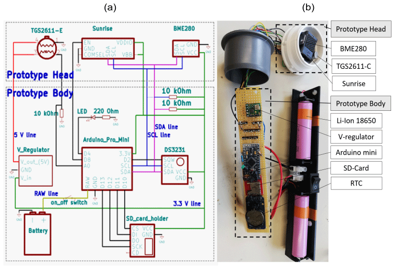
Figure 1 Circuit diagram (a) with the wire connection of the prototype and a picture (b) of the RR prototype. In panel (b), the modules and sensors in the prototype body and the prototype head are highlighted. The membrane, which covers the prototype head, was removed to show the gas sensors.

To continuously record temperature, (relative) humidity and pressure, the BME280 (Bosch Sensortec GmbH, Germany) digital miniature environmental sensor was integrated in the prototype head, with reported operation ranges of −40 to 85 °C, 0 % to 100 % relative humidity (relH) and 300 to 1100 hPa respectively (Sensortec, 2015). Accuracy for the BME280 sensor is ± 1 °C, ± 3 % and ± 1 hPa with a resolution of 0.01 °C, 0.008 % and 0.2 Pa for temperature, relative humidity and pressure respectively (Sensortec, 2015). To measure CO₂ concentration, the Sunrise sensor (Senseair, Sweden) was chosen. This miniature NDIR-type sensor, with an average current consumption of 38 µA, was developed specifically for battery-powered applications. The supply voltage to the sensor can be either 3.3 or 5 V (Senseair, 2019). Manufacturers specify a detection range of 400 to 5000 ppm for CO₂; however, as we turned off the built-in self-correcting automatic-baseline-correction algorithm, measurements down to 0 ppm CO₂ were possible. The Sunrise, the BME280 and the DS3231 RTC communicate with the Arduino Pro Mini via the I2C communication interface, which allows communication between a single primary device and multiple secondary devices through two bus lines. Both lines, the serial data line and the serial clock line, are bidirectional lines, where 1 bit of data is transferred each clock pulse. Both bus lines are connected to the positive pole via 10 kΩ pull-up resistors.

To measure the CH₄ concentration, the TGS2611-E sensor model from the TGS sensor family was selected. The difference between this sensor and other sensors in the aforementioned family is the built-in charcoal filter inside the sensor cap, which reduces the influence of interference gases, such as ethanol or isobutane, and therefore increases the sensor's selective response to methane gas (Figaro Engineering Inc., 2017). The detection range of the TGS2611-E sensor given by the manufacturer is 500–12 500 ppm CH₄, and operating temperature conditions range from −40 to 70 °C. The required voltage supply for the TGS2611-E is 5 V. Therefore, the circuit voltage of the Arduino Pro Mini board was increased from 3.3 to 5 V with a step-up/step-down voltage regulator (S9V11F5S6CMA from Pololu, USA). This voltage regulator provides a constant and accurate circuit voltage (V_C) to the TGS2611-E sensor independent of battery status.

The low-cost TGS2611-E sensor was originally developed to monitor gas quality and possesses a tin dioxide (SnO₂) sensing area, which is heated by a built-in resistive heater. The resistance of the sensor (R_S) changes in the presence of oxidising components, as these react with the oxygen from the sensing film. The change in resistance is measured indirectly as a change in voltage across a reference resistor (R_L) by one of the analogue input pins of the Arduino board. The resolution of the TGS2611-E sensor is therefore defined by the bit depth of the microcontroller. The Arduino possesses a 10 bit analogue-to-digital converter, which enables one to convert an analogue input voltage into a corresponding digital signal of 1024 sampling levels between the common ground and the operating voltage of the board (Beddows and Mallon, 2018). Given the Arduino's operating voltage of 3.3 V, it has a resolution of 3.22 mV per bit. This digital count can be translated into measured voltage at the analogue input pin as follows:

$$\begin{array}{}\text{(1)}& {\displaystyle }{V}_{\mathrm{measured}}=C_{\mathrm{digital}}{\displaystyle \frac{V_{\mathrm{operating}}}{\mathrm{SL}}},\end{array}$$

where C_digital is the digital integer value read by the Arduino, V_operating is the operating voltage of the board and SL is the number of available sampling levels of the analogue-to-digital converter.

The RR prototype is powered by two Li-ion 18650 batteries connected in parallel to sum their capacity. While the negative poles of the batteries were connected to the common ground, the positive poles were connected to the RAW pin using an on–off switch. As this pin is connected to the Arduino's onboard voltage regulator, the RAW pin can be used to supply the board with an unregulated input voltage anywhere from 3.4 to 12 V. The battery voltage of the Li-ion 18650 ranges from 4.2 V in a completely charged state to approximately 3.55 V; therefore, it is always within the supply voltage requirements.

In the design phase of the prototype, the system was assembled using solder-less breadboards. Thus, it was possible to experiment with the circuit design, add components, try different sensors and modify wiring without soldering. The final version was wired on an epoxy board, soldered and fixed on an angled rail. Finally, all components were covered in polyurethane resin (UR5041 Electrolube, UK) to protect the connections from corrosion.

2.2 Methane sensor

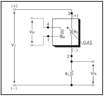
Figure 2 Basic measuring circuit for the TGS2611-E (Figaro Engineering Inc., 2017): the circuit voltage (V_C) and heater voltage (V_H) are 5 V, V_RL is the voltage across the reference resistor, R_H is the heater, R_S is the variable sensing resistor, and R_L is an external resistor. Pins 1, 2, 3 and 4 are the negative pole of the heater, the analogue sensor output, the positive pole of the sensor and the positive pole of the heater respectively.

2.2.1 Methane sensor signal interpretation

The TGS2611-E is connected to the Arduino board (Fig. 2). Pins 3 and 4, the positive pins of the sensor electrode and the heater, are connected to the output of the voltage regulator, which provides a constant 5 V. Pin 1, the negative pole of the heater, is directly connected to the common ground, while pin 2 is connected to an analogue input pin of the Arduino as well as to the common ground via a 10 kΩ resistor (R_L). When a circuit voltage (V_C) is applied to pin 3, the voltage across the reference resistor (V_RL) varies according to the (variable) resistance of the sensing area (R_S) and is measured at pin 2.

Direct conversion of voltage signal to CH₄ concentrations does not generate good enough results (Eugster and Kling, 2012). Therefore, the relative sensor response is calculated as the ratio (R) between the sensor resistance and a reference resistance:

$$\begin{array}{}\text{(2)}& R={\displaystyle \frac{R_{\mathrm{S}}}{R_{\mathrm{0}}}}={\displaystyle \frac{\left(\frac{V_{\mathrm{C}}}{V_{\mathrm{out}}}-\mathrm{1}\right)}{\left(\frac{V_{\mathrm{C}}}{V_{\mathrm{0}}}-\mathrm{1}\right)}},\end{array}$$

where R_S is the sensor resistance at the measured sensor voltage (V_out) and R₀ is an empirical reference resistance at the same temperature and humidity levels in atmospheric CH₄ concentrations. R₀ is obtained from a separate calibration step, which allows one to measure V₀. Using this method, R is less biased towards temperature and humidity influences (Bastviken et al., 2020). In a second calibration step, the CH₄ concentration is computed from the relative sensor response. With this two-step calibration approach, Bastviken et al. (2020) were able to obtain a sensor accuracy of the order of ± 1.1 ppm near typical atmospheric background concentrations. Even though the sensor is not suitable for accurately measuring absolute CH₄ mole fractions at those very low concentration levels, it can be used to monitor relative changes in CH₄ over time if properly calibrated (Bastviken et al., 2020).

Calibration constants were calculated for each prototype individually, as individual sensor calibration is necessary (Riddick et al., 2020). Any differences in the (temporal) response (of the resistance ratio) of identical TGS sensors to CH₄ are attributed to the manufacturing process (Riddick et al., 2020). Previous research on the TGS sensor family has also suggested fitting different calibration equations for the sensor voltage signal to the methane concentration in cold (sub-zero) conditions compared with temperatures above 0°C (Eugster et al., 2020). As we do not expect sub-zero temperatures in the aquatic environments during prototype deployment, sensor voltage readings at temperatures below 0°C are eliminated. Sensor readings with a relative humidity below 40 % are also excluded, as the resistance ratio is not predictable for lower moisture levels (Eugster and Kling, 2012).

2.2.2 Methane sensor calibration in a gaseous headspace

We calibrated multiple methane sensors in a gaseous phase together, following the two-step approach proposed by Bastviken et al. (2020). For both calibration steps, the prototypes were placed in the headspace of a sealed box. The box contained water and was placed in a climatic chamber to allow temperature control. As temperature and humidity co-vary near moist surfaces, alteration of temperature allowed one to vary absolute humidity (absH). Although temperature and absH could not be controlled independently, their variability reflects in situ field conditions in a humid environment. Temperature and relH were continuously recorded by the BME280 sensor integrated in the prototype head. Absolute humidity (in g m⁻³) was calculated from vapour pressure, i.e. from relative humidity, pressure and temperature directly measured in the headspace, according to Vaisala (2013) (detailed computation steps are given in Appendix C). The gas concentration in the headspace was continuously measured by a micro-portable GHG analyser (MGGA; Los Gatos Research, USA) by circulating the gas phase between the analyser and the headspace of the sealed box. The membrane, which is used to cover the prototype head, was removed during calibration measurements in the gaseous headspace to minimise the time lag between the methane sensors and MGGA. A picture of the experimental set-up and a schematic illustration are given in Fig. 3.

The first step of the calibration is needed to compute the reference voltage V₀ for different temperature and humidity levels at background atmospheric CH₄ levels. Therefore, the temperature inside the climatic chamber was continuously decreased from 25 to 5 °C followed by an increase back to starting conditions. Hence, measurement of V₀ over the whole investigated temperature range was possible. Over the period of 2 months, this calibration step was repeated multiple times. Individual experiments lasted between 18 and 30 h, and the measurement interval was set to 30 s. We evaluated four different calibration models from Bastviken et al. (2020), which use different combinations of temperature (T) and absolute humidity (H) as model inputs, and two temperature-only models (Table 2). We used “optim()” (R, version 4.1.1) to optimise model parameters using maximum likelihood. From the six candidate models, we then selected the model that performed best for all prototypes among all individual experiments in terms of maximising the R² value and minimising the root-mean-square error (RMSE). In this step, the calibration models were given data for all calibration experiments except one, and we then used this last experiment to validate our model. This validation step was repeated to validate all models on all calibration experiments and independently for all prototypes. After choosing the best model, the prototypes were individually calibrated using temperature and humidity data from all calibration experiments performed with the respective prototype.

The second calibration step includes the injection of methane gas and the calculation of the CH₄ mole fraction from the sensor resistance ratio. The latter is computed from the raw sensor output (V_out) and modelled V₀ using Eq. (2). The gas concentration was changed by directly injecting calibration gas from a pressurised gas bottle (Air Liquide, Austria). The use of dry standard gas, with only a few parts per million of H₂O, is discouraged, as it drastically decreases the relative humidity (Riddick et al., 2020). Therefore, we used pumice stones, normally used in fish tanks, to bubble the dry standard gas through the water column and were thereby able to maintain a relative humidity above 50 %.

Calibration gas contained 50 ppm CH₄ and 10 000 ppm CO₂ (± 2 % uncertainty for both gases), and gas addition was controlled by a pressure valve. Methane was injected in a step-wise manner and the concentration increased gradually starting from the atmospheric background. Over the period of 3 months, this experiment was repeated multiple times. Individual experiments lasted between 2 and 6 h, and the measurement interval was set to 1 s. As both the gas concentration and the TGS2611-E sensor output were continuously recorded by the MGGA and the prototype respectively, we could directly relate these two measurements.

The five most successful models proposed by Bastviken et al. (2020) were used to compute CH₄ concentration (Table 3). Used metrics for model selection were the R² value and the RMSE between the modelled methane concentration and the measured concentration by the MGGA. To choose the best model, the same procedure as for V₀ model selection was used. Finally, prototypes were individually calibrated using data from all calibration experiments performed with the respective prototype.

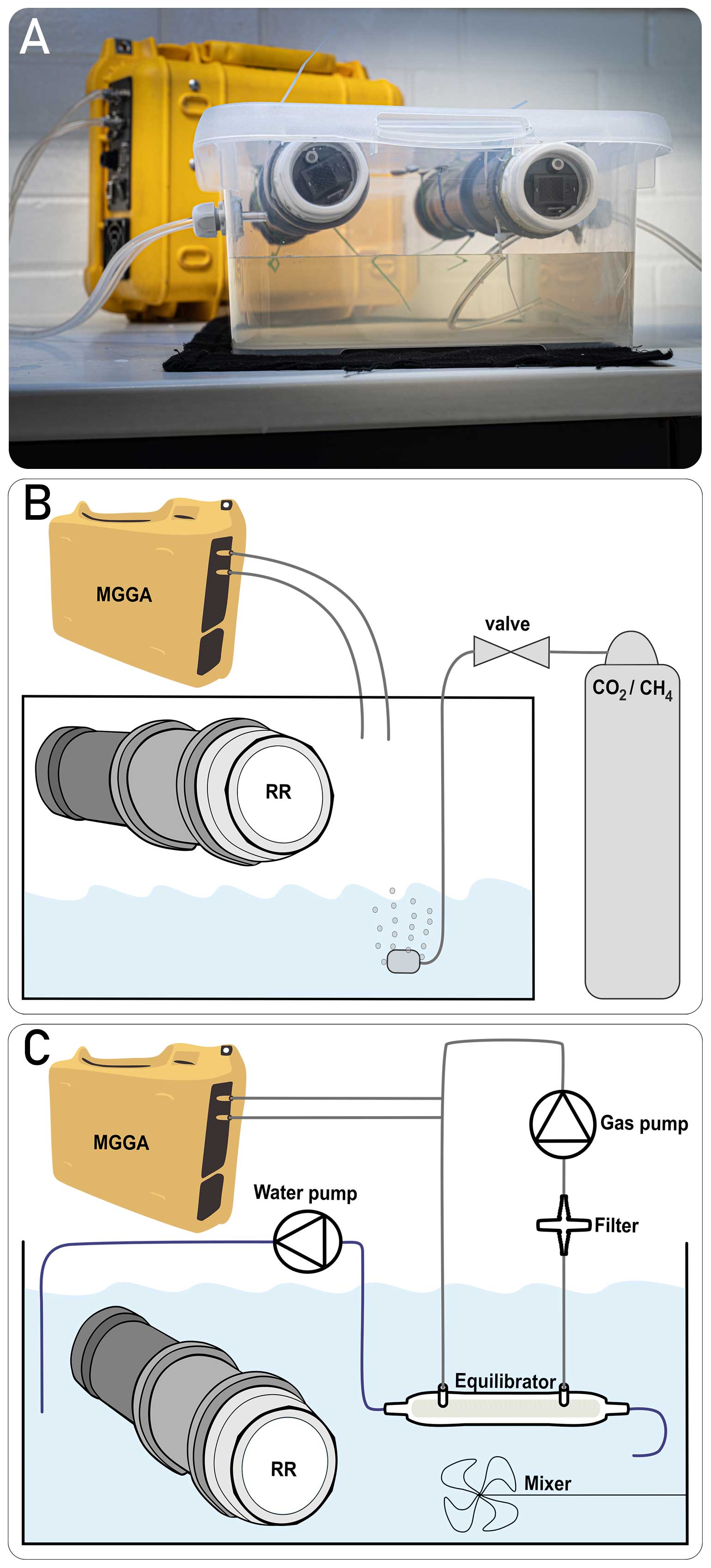
Figure 3 Experimental set-up of the CH₄ sensor calibration: picture (a) and schematic illustration (b) of calibration in a gaseous headspace and  (c) schematic illustration of calibration submerged in water. For the latter, the gas loop is shown with grey lines and the water tubes with purple lines.

2.2.3 Methane sensor calibration submerged in water

To create close-to-reality measurement conditions and to evaluate the gas sensors for in situ measurements, the prototype head was covered by the membrane and submerged in water. To ensure equilibration with the background during reference voltage computation, the water was bubbled with background air using pumice stones for at least 12 h prior to prototype deployment. The set-up was placed in the climatic chamber to allow for temperature control, and the temperature was varied between 5 and 25 °C. Continuous change in temperature allowed one to measure V₀ over the whole investigated temperature range. Over a period of 1 month, the experiment was repeated multiple times. Individual experiments lasted between 5 and 10 h, and the measurement interval was set to 3 s. Model selection and calibration was done according to the same procedure as for the headspace calibration.

Figure 4 Senseair Sunrise pin configuration (a) and connection diagram (b) for the I2C communication between the Senseair Sunrise sensor and any host system (Senseair, 2019).

For the second calibration step, the prototypes were placed in different waterbodies that had a gradually increasing methane concentration. This gradient was achieved by various dilution steps of a highly concentrated water phase (with approximately 2200 ppm CH₄), which was extracted from a nearby hypertrophic pond. The MGGA was again used as the reference instrument to measure the methane concentration in the water by equilibrating a closed gas loop with the water phase. For this, water was pumped continuously (0.5 L min⁻¹) through a membrane-based equilibrator (MiniModule membrane contactor, 3M, Germany). The equilibrator uses a hollow-fibre membrane, where water flows inside the fibres and the gas flows on the outside to ensure maximum gas exchange efficiency. The gas phase is continuously circulated in the opposite direction to the water phase using a membrane pump (at approximately 2 L min⁻¹). From the gas loop, a gas sample is bypassed through the MGGA to measure the concentration of the gas phase. A hydrophobic filter is installed before the gas pump to protect the devices from water. Equilibration between the two phases is expressed as plateauing measurements of the MGGA. The mean value of a 10 min long plateau was used as reference concentration for calibration. To prevent a change in the CH₄ concentration over time, the set-up was placed in a gas-tight box; to prevent a concentration gradient in the water phase, it was continuously mixed using a pump. The experimental set-up is illustrated in Fig. 3

The whole set-up was placed in a climatic chamber to maintain a constant temperature during experiments. We conducted CH₄ calibrations at temperatures of 8, 15 and 25 °C. Over the period of 1 month, the experiment was repeated multiple times with various concentrations of CH₄ in the water phase. Measurements at each specific CH₄ and temperature level lasted at least 40 min, and the measurement interval was set to 1 s. We took the average from the sensor readings recorded during stable sensor response at a specific CH₄ and temperature level to calibrate the TGS2611-E sensor against the (mean) concentration measured by the MGGA. Model selection and calibration was done according to the same procedure as for the headspace calibration.

From the equilibrated headspace concentration measured by the TGS2611-E sensor (in ppm), the dissolved gas concentration (C_CH4,W in mol L⁻¹) can be computed by applying Henry's law of solubility:

$$\begin{array}{}\text{(3)}& C_{\mathrm{CH}\mathrm{4},\mathrm{W}}=p_{\mathrm{CH}\mathrm{4}}\cdot {\mathrm{KH}}_{\mathrm{CH}\mathrm{4}}\left(T_{\mathrm{W}}\right),\end{array}$$

where p_CH4 is the partial pressure (in atm) of CH₄ and computed as the product of the equilibrated molar fraction of CH₄ measured by the TGS2611-E sensor and the pressure measured by the BME280. KH_CH4 (in mol L⁻¹ atm⁻¹) is the gas-specific, temperature-dependent Henry constant and can be calculated for every water temperature with parameterisation from IHA (International Hydropower Association, 2010, as shown in Appendix D). Water temperature was approximated using the temperature measured by the BME280.

2.3 Carbon dioxide sensor

2.3.1 Carbon dioxide sensor set-up

To measure CO₂, the Sunrise sensor from Senseair is used. The Sunrise is connected to the Arduino board (Fig. 4). The Sunrise VDDIO and VBB pins are connected to the VCC pin of the Arduino, which provides 3.3 V, and the COMSEL pin and the GND pin are connected to the common ground. The I2C communication pins are connected to the respective bus lines, and the Sunrise EN pin is connected to Arduino’s digital pin 8. In the Arduino sketch, pin 8 is defined as output and set to high.

An Arduino sketch used for configuration of the Sunrise sensor is needed to change the I2C address. Every I2C address contains 7 bits and needs to be unique in a system. As the default address for both the Senseair Sunrise and the RTC DS3231 are the same (0×68), one of them needs to change in order to operate both modules on the same primary device. Additionally, the measurement mode is set to single mode in order to trigger a measurement on the host's command, and the automatic baseline correction function is disabled. This function, which is installed on the Sunrise sensors by default, corrects for sensor drift, thereby making sensor calibration dispensable and extending sensor life. The function takes the lowest recorded value during an 8 d interval and automatically sets it to 400 ppm CO₂. This comes in very handy when the sensors are used indoors, where it is safe to assume that the lowest recorded value during this interval corresponds to fresh air. However, for the purpose of our prototypes this assumption is not valid, as freshwater may also be undersaturated in terms of CO₂. As the automatic baseline correction function is disabled, the sensors have to undergo a target gas calibration.

Senseair also implemented a software algorithm to correct the CO₂ readings for temperature and pressure fluctuations. However, pressure compensation was deactivated for measurements with the RR prototypes; thus, Sunrise readings had to be corrected for the measured pressure level. Deviation is 1.58 % of the reading per kilopascal deviation from mean sea-level pressure (Senseair, 2019). Pressure from the BME280 is used to correct the CO₂ values. Thus an eventual increase in pressure due to higher hydrostatic pressure, e.g. when measuring in deep water, is also taken into account.

2.3.2 Carbon dioxide sensor measurements

We did a zero calibration with pure N₂ to set the origin of the sensors. Afterwards, calibration was verified by exposing the sensors to two different calibration gas standards (Air Liquide, Austria) with CO₂ concentrations of 350 and 10 000 ppm respectively. Additionally, the gas concentration was continuously recorded with the MGGA, which was operated in parallel and used as the reference instrument.

As the standard gas used for the second step of the methane sensor calibration in the headspace (Sect. 3.1.1) contained 10 000 ppm CO₂ and the concentration was increased continuously, these experiments were used to verify calibration within the whole measurement range and to evaluate the influence of humidity and temperature variations on the Sunrise sensor readings. Furthermore, as these measurements were conducted between 9 and 23 months after the sensor calibration, assessment of the long-term behaviour of the sensor was possible. Measurements of the Sunrise sensor were again compared with measurements from the MGGA, which was used as the reference instrument.

To validate in situ performance of the CO₂ measurements, we deployed the prototypes for 24 h in a nearby natural stream to measure diurnal fluctuation in dissolved CO₂. After pressure correction of the Sunrise sensor readings, the dissolved gas concentration (C_CO2,W, in mol L⁻¹) was computed by applying Henry's law of solubility (Eq. 3). The partial pressure of CO₂ in the headspace was calculated from Sunrise sensor readings, and the pressure was measured by the BME280. The Henry constant was computed with a specific parameterisation for CO₂ (reported in Appendix D) at temperatures measured by the BME280. Thereby the computed dissolved CO₂ concentration was compared with discrete grab samples taken at random times during prototype deployment. Those samples were taken using the headspace technique and measured using the MGGA in a closed-loop configuration (Wilkinson et al., 2018). Samples were taken with a syringe by collecting 70 mL of water and background air respectively. The concentration of the latter was additionally measured with the MGGA. To enhance equilibration between the two phases, the syringe was intensely shaken for approximately 2 min. The gaseous headspace was then transferred into pre-evacuated gas vials and stored with over-pressure until further analysis. This closed-loop method requires consideration of sample dilution by ambient gas (Dalvai Ragnoli et al., 2023). For this purpose, a sample of gas standard with known gas composition was analysed under in situ pressure and temperature conditions to calculate a volume ratio between the sample and loop volume (Dalvai Ragnoli et al., 2023). From the resulting headspace concentration, the equilibrium concentration of the water phase was computed using Henry's law of solubility. The original water concentration was finally computed by summing the number of moles in the equilibrated phases and accounting for the background concentration.

3 Results and discussion

3.1 Methane sensor calibration

3.1.1 Calibration in a gaseous headspace

The two-step calibration was first done in a gaseous phase to evaluate the sensor's suitability to measure the methane concentration. For the first step of the calibration, the temperature (and thereby absolute humidity) was varied in order to model V₀ over the wide range of ambient conditions expected in freshwater environments. The continuous change in temperature during the calibration experiments resulted in a continuous gradient in absolute humidity. Temperature was varied between 6 and 25 °C, and mean relative humidity in the prototype head was 76 ± 3 % on average among prototypes, resulting in an absolute humidity ranging from 4 to 19 g m⁻³. At the background atmospheric CH₄ concentration, the measured output voltage of the sensor (V_out) corresponds to V₀ and, for all sensors, the voltage signal increased linearly with increasing temperature and humidity (Fig. 5a).

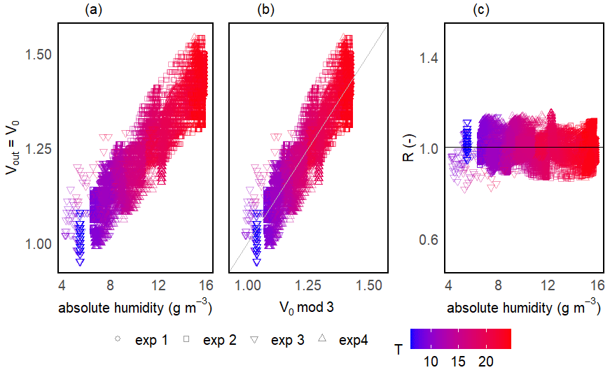
Figure 5 Sensor voltage signal vs. absolute humidity and temperature for one of the prototypes during V₀ calibration experiments (a). Measured vs. modelled V₀ using V₀ mod 3 (b) and resistance ratio vs. absolute humidity and temperature (c). Different symbols represent independent calibration experiments and the colour gradient shows the respective temperatures. The grey line in panel (b) represents the 1:1 line and the black horizontal line in panel (c) represents mean R for this prototype. Note that the variance on the y axis is due to the inherent noise in the sensor signal.

The model selection step resulted in the simple linear model using the absolute humidity as the predictor (V₀ mod 3) having the highest R² and lowest RMSE for all prototypes; therefore, it was chosen to compute V₀. The same linear model was used by Bastviken et al. (2020) to compute V₀, because of the combination of best fit and minimum number of parameters. A summary of the performance of all six V₀ model candidates is provided in Table 2. Model parameters are sensor-specific for every prototype and reported in Table 6.

Models using relH instead of absH have been reported (Bastviken et al., 2020) to return lower R² values; therefore, they were not taken into account in this calibration step. Using absH instead of relH was also suggested by Eugster et al. (2020), who were thereby able to reduce typical deviation from the reference to less than ± 0.1 ppm CH₄. The better prediction when using absH can be explained by the fact that the sensing area reacts with the absolute number of water molecules in the sensor head, which compete with other molecules for space on the active sensor surface (Eugster et al., 2020). Models that include temperature as a predictor had lower R² values when comparing predicted and modelled V₀, indicating that the temperature effect is negligible compared to absH. Previous studies (Bastviken et al., 2020) attribute this to the heating power (280 mW; Figaro Engineering Inc., 2017) of the built-in resistive heater.

Unlike the raw voltage signal, R is independent of temperature and humidity (Fig. 5c). At the background atmospheric methane concentration, R was always very close to 1 for all prototypes (1.00 ± 0.11, 1.00 ± 0.05 and 1.00 ± 0.05 for prototypes RR1, RR2 and RR3 respectively) throughout the whole investigated temperature and humidity range (Table 4). It can be concluded that changes in sensor response induced by changing environmental factors can be successfully corrected.

Table 2 Results of the V₀ model validation: R² and RMSE are averaged over the number of experiments (N) and n is the total number of measurement points used for calibration. V₀ mod 1–4 are models proposed by Bastviken et al. (2020). V₀ mod 5 and V₀ mod 6 are temperature-dependent models and were added, as proven necessary, during this study. The unit of V₀ is voltage, T is the temperature (°C) and absH is the absolute humidity (in g m⁻³). Models using relH instead of absH are not taken into account, as they return lower R² values (Bastviken et al., 2020). Model parameters g, h, m, n and S are sensor-specific constants and are derived from curve fitting. Note that unit for RMSE is volts.

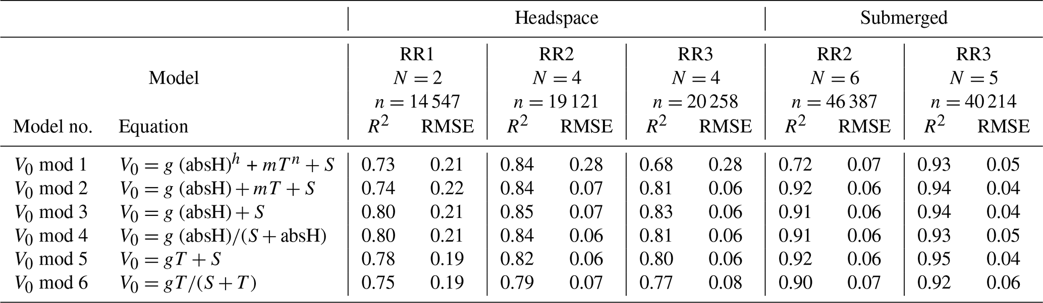
Table 3 Results of the CH₄ model validation: R² and RMSE are averaged over the number of experiments (N). For the headspace calibration, n is the total number of measurement points used for calibration. For the submerged calibration, n is the number of specific temperature and CH₄ levels used for calibration. No CH₄ calibration experiments were performed with RR1. For the submerged calibration, sensor readings are averaged during stable sensor response at each specific temperature and CH₄ level. CH₄ is in units of parts per million, R is the resistance ratio of $\frac{R_{\mathrm{S}}}{R_{\mathrm{0}}}$, T is the temperature (°C), and relH and absH are the relative and absolute humidity in percent and grams per cubic metre respectively. Model parameters a, b, c, d, e, f and K are sensor-specific constants and derived by curve fitting. Note that unit for RMSE is parts per million of methane (ppm CH₄).

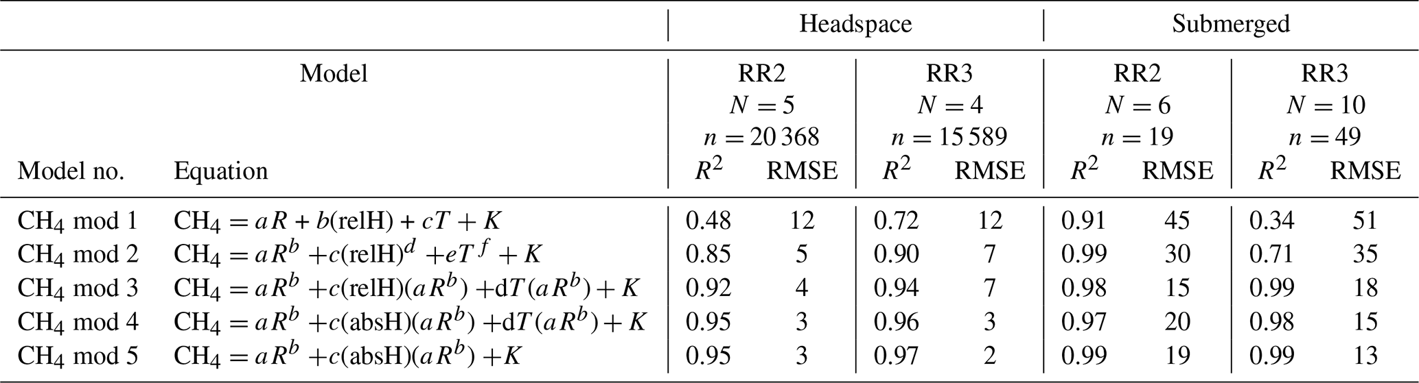
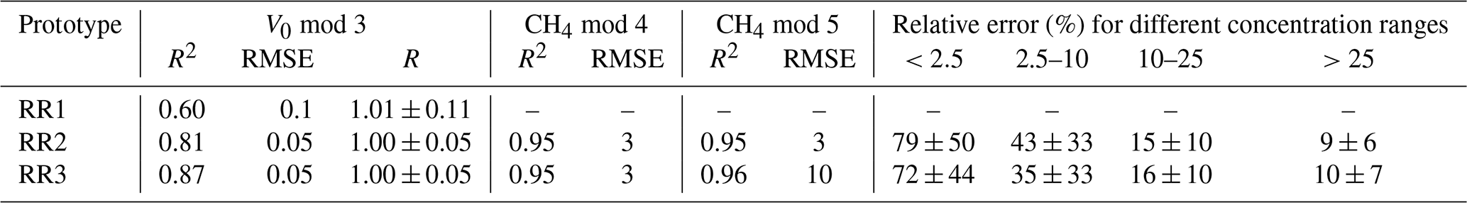
With an increasing methane concentration, the sensor voltage signal V_out also increased. As the temperature and humidity were kept stable during these measurements, thereby keeping V₀ constant, R decreased with an increasing methane concentration (Fig. 6). Models using relative humidity instead of absolute humidity to predict CH₄ resulted in lower R² values and higher RMSE values, as absH was again the most important predictor. A summary of the performance of all model candidates is provided in Table 3. Bastviken et al. (2020) chose V₀ mod 3 in combination with CH₄ mod 5 as a compromise between a good fit and the minimum number of parameters and were thereby able to predict the CH₄ concentration to ± 10 ppm in the range from near-ambient concentrations to 719 ppm CH₄. We computed the molar fraction of CH₄ using CH₄ mod 4 and CH₄ mod 5 separately and obtained the best results using the combination of V₀ mod 3 with the slightly more complex CH₄ mod 4 model. Using this combination, we were able to compute CH₄ with an absolute error of ± 3 ppm in the range of 2 to 45 ppm CH₄ for both prototypes (Table 4). However, near the atmospheric background concentration (<2.5 ppm CH₄), our model predictions have the highest offset to measured values with relative errors of 79 % and 72 %, corresponding to 3 ± 2 and 4 ± 1 ppm CH₄, for prototype RR2 and RR3 respectively. With an increasing CH₄ concentration, the relative error of our model prediction decreased considerably (Table 4), which indicates that measurements of absolute CH₄ concentration with the TGS2611-E sensor have to be taken with caution, especially in the low-concentration range. This is not unexpected, as the detection limit of this cheap metal oxide sensor is reached. However, the TGS2611-E sensor is reasonably able to measure CH₄ concentrations above 10 ppm. Calibration parameters of our prototypes for measurements in the gas phase are reported in Table 6.

Table 4 Results of the model prediction for the TGS2611-E sensor in the gaseous headspace. Shown are the regression metric R² and the RMSE for sensor calibration using all calibration experiments for each calibration step. The resistance ratio R is reported as the mean ± standard deviation for all measurements at a background atmospheric CH₄ concentration. Note that the unit for the RMSE during V₀ calibration is volts, whereas the unit for CH₄ calibration is parts per million. The mean relative error and the standard deviation (in %) of model prediction using the combination of the V₀ mod 3 and CH₄ mod 4 are shown for different concentration ranges (in ppm CH₄).

Due to the experiment run time exceeding the battery lifetime for some measurements during V₀ calibration, the sensor did not always manage to measure over the full calibration cycle. Therefore, the sensor only occasionally managed to measure during the temperature increase back to starting conditions following the previous temperature decline in the climatic chamber. Whenever the sensor did manage to measure the complete cycle, a hysteresis effect in the sensor voltage signal was observed: during the heating process, the voltage signal was consistently higher than during the cooling process for the same temperature and humidity conditions (Fig. 7). We interpret this hysteresis as a result of the time lag between temperature and humidity in the headspace of the calibration box. This hysteresis effect was not included when considering equations to model V₀, as it would require one to assess the history of the measurements. However, as the hysteresis effect is not accounted for in the modelled V₀, the hysteresis is dragged into the resistance ratio and, thus, expectedly reduces model accuracy (Fig. 7).

3.1.2 Calibration submerged in water

To simulate equilibration between the water phase and ambient air, and thus measure V₀ when the prototypes are submerged, ambient air was bubbled through the water column. To ease the use of the RR prototype for future users, we first checked if parameters obtained in the quite easily achievable headspace calibration can be directly used for underwater measurements. However, applying V₀ mod 3 and the parameters obtained from the headspace calibration on the submerged prototypes resulted in an offset between predicted and measured V₀: although modelled V₀ was still highly linear to measured V₀ (R² values of 0.91 and 9.94 for RR2 and RR3 respectively), and therefore indirectly to (absolute) humidity and temperature, the sensor featured an offset in the form of a parallel shift (RMSE values of 0.13 and 0.09 mV for RR2 and RR3 respectively). Thus, the resulting overestimation of the resistance ratio of, depending on the prototype, 8 % or 13 %, finally results in an overestimation of the CH₄ concentration. Although the relative change in the CH₄ concentration, for example, over time, could be assessed using transferred calibration parameters, more accurate measurements of absolute CH₄ concentration are not feasible. We conclude that parameters from calibration in a headspace can be used for submerged measurements if the user does not have the equipment to perform the more complex calibration underwater or if measurements of the relative change in dissolved CH₄ concentration are sufficient. However, to measure absolute concentration, we suggest performing a separate calibration under in situ conditions. Performing this labour-, time- and equipment-intensive calibration decreases measurement error and increases measurement accuracy.

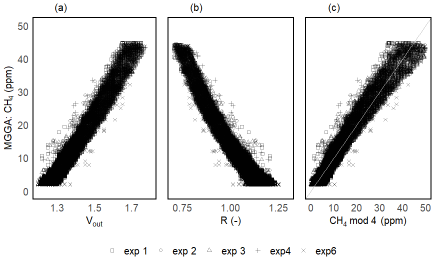
Figure 6 Results for the headspace CH₄ calibration step for one of the prototypes: sensor voltage signal (a), resistance ratio (b) and modelled CH₄ (using CH₄ mod 4, c) vs. the CH₄ concentration measured with the MGGA as the reference instrument. Different symbols represent individual calibration experiments. The grey line in panel (c) represents the 1:1 line.

Following the same procedure for model selection used for the gaseous headspace calibration resulted in V₀ mod 2 and V₀ mod 5 being the best models to compute V₀ in a submerged environment (Table 2). Both models use temperature as a model predictor, indicating a stronger temperature influence on the sensor output for submerged prototypes compared with measurements in air. We have two not necessarily exclusive explanations for this behaviour. First, the lower importance of humidity compared with measurements in air can result from stable humidity conditions in the prototype head. Although humidity was on average higher during submerged measurements, it could quickly equilibrate through the membrane and experienced less variation compared with measurements in the gaseous headspace. While the temperature varied from 26 to 8 °C, the mean relative humidity in the prototype head was 87 ± 4 % and was never below 56 %. Second, the physical properties of the medium surrounding the prototype may play an important role, as thermal conductivity for air is an order of magnitude lower than for water; therefore, heat transfer in the water phase much faster. Thus, the resulting higher rates of heat dissipation in the water make temperature a dominant factor on the resistance of the TGS2611-E sensor.

As a compromise between the best fit (high R² and low RMSE) and the lowest number of parameters, we selected V₀ mod 5 to compute V₀ for submerged measurements. Using this model, the resistance ratio was close to 1 in the whole investigated temperature range with very little deviation (1.00 ± 0.06 and 1.00 ± 0.06 for prototypes RR2 and RR3 respectively; Table 5).

The second calibration step was performed at three different temperatures (8, 15 and 25 °C) and with dissolved CH₄ concentrations ranging from 0.01 to 0.3 µmol L⁻¹. The temperatures and concentration range were chosen in order to represent ranges typically found in freshwater ecosystems (Stanley et al., 2016; Flury and Ulseth, 2019; Dalvai Ragnoli et al., 2023). The dissolved CH₄ concentration was computed using Eq. (3) and by approximating the water temperature with the temperature measured by the BME280 in the prototype head. As the conversion from the molar fraction measured in the prototype head to the dissolved gas concentration is a mathematical operation and as our aim is to convert the voltage reading of the TGS2611-E sensor to the more typically reported molar fraction (ppm), we report our calibration results in parts per million hereafter, rather than in moles per litre.

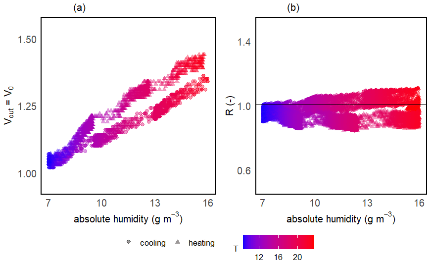
Figure 7 Observed hysteresis in the sensor voltage signal during the V₀ calibration step (a) and the resulting resistance ratio using the simple linear V₀ mod 3 model (b). The colour gradient shows respective temperatures. The black line in panel (b) represents mean R for this prototype.

Table 5 Results of the model prediction for the TGS2611-E sensor submerged in water. Shown are the regression metric R² and the RMSE for sensor calibration using all calibration experiments for each calibration step. The resistance ratio R is reported as the mean ± standard deviation for all measurements at a background CH₄ concentration. Note that the unit for the RMSE during V₀ is parts per million. The mean relative error and standard deviation (in %) of model prediction using the combination of the V₀ mod 5 and CH₄ mod 5 are shown for different concentration ranges (in ppm CH₄).

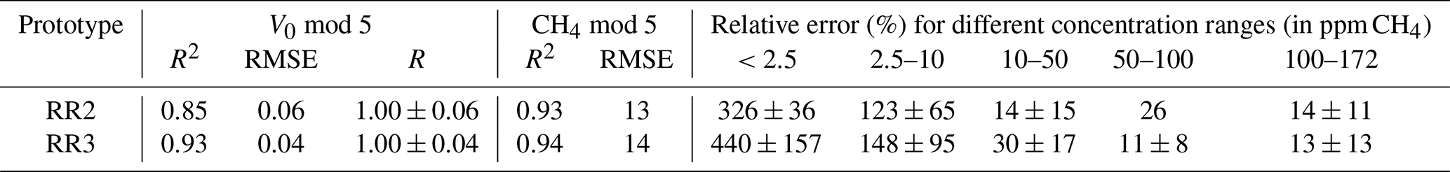
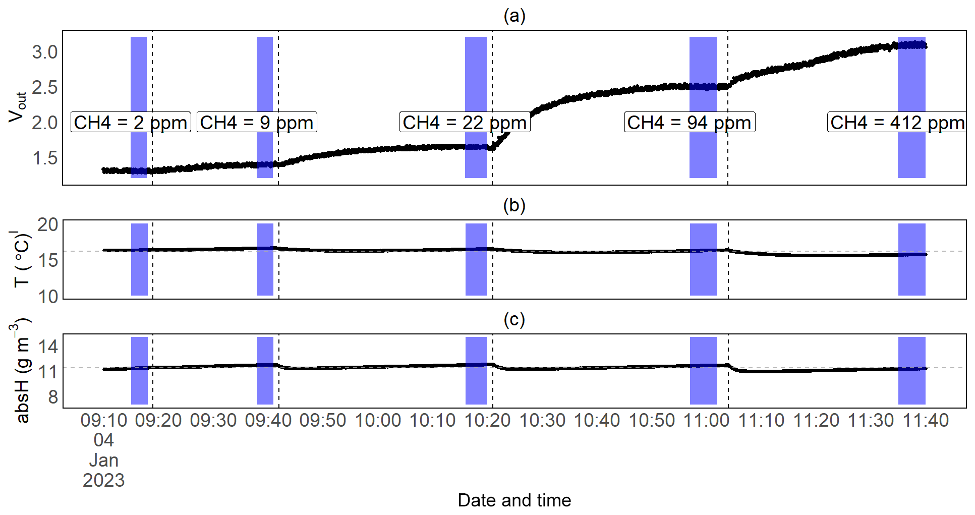
Figure 8 Time series measurement for one of the submerged CH₄ calibration experiments: the raw voltage output signal from the TGS2611-E sensor (a), temperature (b) and absolute humidity (c) over time. The vertical dotted lines represent the moments when the prototypes were submerged in a new (higher) CH₄-concentrated water phase, and the purple fields represent the time interval of stable measurements during which we took the average of the sensor readings to calibrate the TGS2611-E sensor against the (mean) concentration measured by the MGGA. The latter are shown for this experiment in panel (a). Horizontal dotted lines in panels (b) and (c) represent the mean temperature and humidity values for this experiment.

Submersion in a methane-enriched water phase resulted in a voltage increase at constant temperatures, resulting in a drop in the resistance ratio (Figs. 8; 9a, b). On average, it took about 30 min for the voltage signal to stabilise after submerging the prototypes in a higher-concentration water phase (with an average CH₄ increase in the water phase of 35 ppm). The extent of the concentration difference between the two water phases does affect the duration until equilibration is reached between the new water phase and the prototype head. Thus, it also affects sensor response time. However, we did not systematically investigate the sensor response time, as data from our experiments do not allow this. The model selection for CH₄ resulted in CH₄ mod 3, 4 and 5 giving the best results (Table 3). Using CH₄ mod 5 as combination of the best fit and minimal number of parameters, we were able to predict CH₄ with an accuracy of 13 and 14 ppm in the range from 2 to 172 ppm CH₄, and our model results were highly linear to measured CH₄ in the water phase (R² of 0.93 and 0.94 for RR2 and RR3 respectively; Table 5).

The error in the CH₄ prediction was highest at concentration levels near the atmospheric concentration until up to 10 ppm CH₄ (with the relative measurement error always higher than 100 %; Table 5). Here, the model overestimates the CH₄ concentration on average by 9 ppm at near-atmospheric concentrations (<2.5 ppm CH₄) and by 7 ppm in the concentration range from 2.5 to 10 ppm CH₄. This is a result of reaching sensor detection limits, where cross-interference with temperature and humidity are experienced more strongly. At higher methane concentrations, the influence of cross-interference is weaker and the contribution of CH₄ to the sensor resistance is stronger. As a result, methane concentration measurements in higher-concentration environments were more accurate.

Measurement error, especially in the low-concentration ranges, was always higher when the prototypes were submerged in water compared with measurements in air: while the relative error near the atmospheric background was 79 % and 72 % in air, the error was 326 % and 440 % in the water phase for prototypes RR2 and RR3 respectively. While measurements in the low-concentration range have to be taken with caution, the low-cost TGS2611-E sensor can be used to measure CH₄ with reasonable accuracy at higher concentration ranges (above 10 ppm CH₄). The calibration parameters of our prototypes for measurements in water are reported in Table 6.

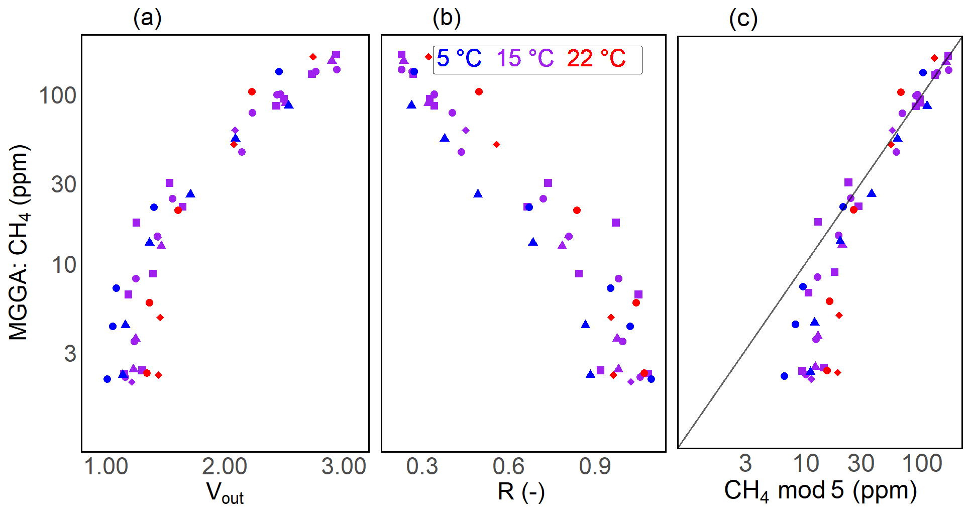
Figure 9 Results for the CH₄ calibration step for one of the submerged prototypes: sensor voltage signal (a), resistance ratio (b) and modelled CH₄ (using CH₄ mod 5, c) vs. the measured CH₄ concentration with the MGGA as the reference instrument. Different symbols represent individual calibration experiments, colours show the temperature during calibration experiments and the black line in panel (c) represents the 1:1 line. Note that the vertical axes and the horizontal axis of panel (c) are on a logarithmic scale.

These experiments, and thus our sensor validation, were performed during a relative short time period of months and sensor drift effects were excluded. However, intense usage of these metal oxide sensors can result in material corrosion and sensor drift, especially if used in harsh and humid environments like those reported in this study. With our current data, long-term sensor drift in submerged environments cannot be predicted. However, previous work with sensors from the TGS sensor family has reported a sensor drift of less than 1 ppm CH₄ yr⁻¹ in air (Eugster and Kling, 2012; Collier-Oxandale et al., 2018; Eugster et al., 2020). Eugster et al. (2020) further calculated that these sensors might reach the end of their lifespan after approximately 10 years based on the downward drift of the voltage signal. Moreover, intense exposure to highly oxidising environments and harsh conditions can decrease the lifetime of the sensors.

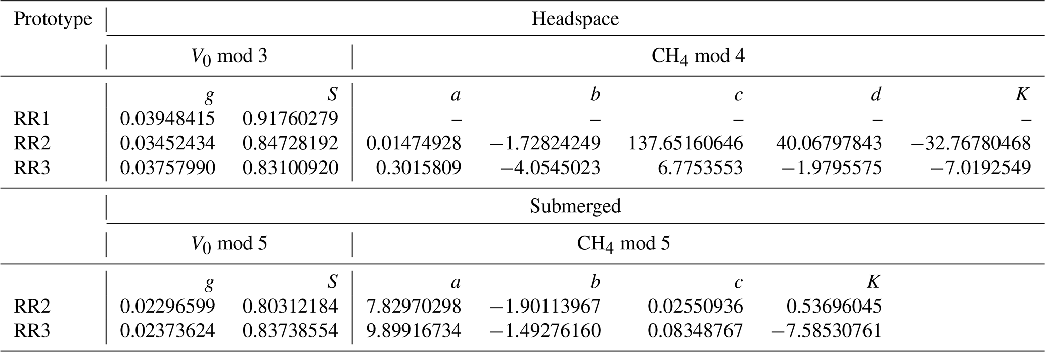
Table 6 Calibration parameters for River Runner prototypes. Here, only parameters for respective best model combinations are presented for measurements in air (V₀ mod 3 and CH₄ mod 4) and for measurements underwater (V₀ mod 5 and CH₄ mod 5). Model parameters are sensor-specific.

3.2 Carbon dioxide sensor

After performing the zero calibration in pure nitrogen, the Senseair Sunrise sensors were exposed to a closed atmosphere with 0, 350 and 10 000 ppm CO₂. After pressure correction, the R² value between Sunrise sensor readings and the measurement of the reference instrument was always higher than 0.99 using at least 85 single measurements (Table 7).

Table 7 Results of Senseair calibration: R² values of the linear regression between the Sunrise sensors and the reference instrument during calibration, RMSE values between the Sunrise sensors and the reference instrument during headspace calibration of the methane sensor, and number of measurements (N) used to compute the RMSE. The relative error of sensor reading for different concentration ranges is given as the mean ± standard deviation.

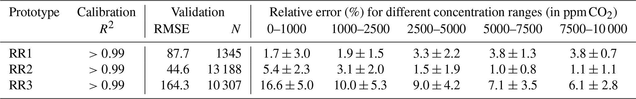
A total of 9–23 months after sensor calibration, the sensor performance was investigated in a wide temperature and humidity range (temperature 15–29 °C and relH 7 %–93 %) during methane sensor calibration (Fig. 10). Using the RMSE as a measure of sensor accuracy, we managed to measure CO₂ with an absolute error of ± 87 ppm for RR1, ± 44 ppm for RR2 and ± 164 ppm for RR3 in the range from 400 to 10 000 ppm CO₂.

Figure 10 Calibration and long-term evaluation of prototypes RR1 (a), RR2 (b) and R3 (c). Calibration is shown in blue: dots represent measurement points and the blue line represents the linear regression between the sensor and reference instrument. Grey symbols represent measurements during evaluation experiments. Different symbols illustrate independent validation experiments and the grey line represents the 1:1 line.

The absolute error between measurement of the Sunrise sensor and the reference instrument increases linearly with the CO₂ concentration for all sensors. However, the slope of the linear relationship differs among sensors. As a difference in the wiring does not influence sensor readings, sensor behaviour characteristics might stem from variations in sensor manufacturing or from contamination of the main components (e.g. infrared source, filter, and infrared detector). The relative measurement error does not show a clear trend among prototypes and exceeds the 10 % boundary only once for RR3 in the low-concentration range (Table 7).

No correlation between elapsed time since sensor calibration and absolute measurement error of the Sunrise sensors was found (R² of 0.39), indicating that even after up to 23 months and extensive exposure to temperature and humidity variations, no post-correction of the Sunrise sensor readings was needed. However, we do recommend resetting the origin of the sensors at times, especially as the effort involved in this step is minor.

Figure 11 In situ CO₂ measurements for one of the RR prototypes. Black dots are the dissolved CO₂ concentration computed with the readings from the Sunrise sensor and Henry's law of solubility. Blue dots represent the mean of grab samples taken in duplicate with the headspace method at discrete times. The standard deviation of these measurements is shown with the error bar. The grey line represents the equilibrium concentration with the atmosphere and was computed from the background concentration and temperature measured by the BME280 using Henry's law of solubility.

With our prototype, we were able to measure the diurnal concentration dynamics of CO₂ in a natural stream in situ. Measurements from our prototype resulted in a slightly lower dissolved gas concentration than computed from the discrete headspace samples taken at arbitrary times. The mean concentration difference between the two measurements was 17 ± 11 µmol L⁻¹ and was highest for the measurements at a high CO₂ concentration. Here, measurements with our prototype resulted in 63 µmol L⁻¹ compared with 90 µmol L⁻¹ from the discrete gas sample. While variance from our sensor signal is small, it is worth noting that deviation in independently but simultaneously taken headspace samples can be notable. The maximum deviation from our grab samples taken at the same time was 38 µmol L⁻¹ (Fig. 11). This is a result of the error-prone nature of this sampling method. The CO₂ concentration over the investigated time period varied by 11 %, which equals a maximum concentration difference of 23 µmol L⁻¹. The water phase was always supersaturated in CO₂ compared with the atmospheric equilibrium (Fig. 11), and, unsurprisingly, the CO₂ concentration was higher during nighttime when photosynthesis is absent and respiration prevails. To capture these daily dynamics with discrete grab samples would require a high sampling frequency; thus, it is a very labour-intensive process. In contrast, our prototype allows one to uncover temporal variability at high resolution with almost no effort.

4 Conclusions and outlook

In the future, we expect cheap self-built sensors, like the presented River Runner prototype, to help to identify and quantify sources of GHG emissions and to deliver robust measurements to improve global flux estimates. Especially in freshwater ecosystems, where accurate (average) measurements are particularly difficult to achieve due to spatial heterogeneity and temporal variability, our prototype can be used for continuous measurements of dissolved CH₄ and CO₂ concentrations. By using a larger set of replicate sensors in a distributed sensor network, the challenges of spatial heterogeneity and temporal variability may be addressed simultaneously, e.g. at various points across a river network or as a series of sensors aligned vertically to measure depth gradients in lakes and reservoirs. To date, such approaches have simply not been possible or have been limited by the high equipment cost. The low cost of the presented prototype makes such endeavours financially feasible.

Our main findings can be summarised as follows:

• The River Runner. We successfully combined an Arduino Pro Mini microprocessor board with a real-time clock; a microSD card adapter; a voltage regulator; a sensor for humidity, pressure and temperature; and gas sensors for CH₄ and CO₂. The measurements from the different sensors are saved on the SD card, and the measurement interval is definable by the user. The total material cost was less than EUR 200. The prototype head was covered with a gas-permeable membrane to allow equilibration between the water phase and a confined gaseous headspace, thereby permitting one to measure dissolved gas concentrations in situ. The membrane of our choice is made of PTFE with a thickness of 0.25 mm and shows a good compromise between gas diffusivity, liquid entry pressure and mechanical strength. Absolute humidity inside the prototype head was computed from vapour pressure, i.e from the pressure, relative humidity and temperature measured by the BME280 sensor. For freshwater, the molar fraction measured in the headspace (in ppm) can be directly converted to dissolved gas concentration (in µmol L⁻¹) using Henry's law of solubility combined with pressure and temperature readings from the BME280 sensor. The accuracy of this conversion could be increased by including a resistance thermometer, which is waterproof and can measure water temperature directly. We did not systematically investigate the sensor response time. However, the sensor response time is tied to the equilibration time between the sensor headspace and the water phase and, thus, is accelerated by further minimising the headspace volume or by maximising the membrane surface.

  With the use of two Li-ion 18650 batteries, continuous measurements with an interval of 30 s were possible for approximately 24 h. However, decreasing the measurement frequency can prolong the battery lifetime. An additional software-based option to consider in order to minimise power consumption is the use of the Arduino Sleep Mode (Beddows and Mallon, 2018). This function temporarily turns the Arduino off completely. However, the TGS2611-E sensor, which in our current assembly is the most power-intense module, would need to be constantly heated to provide reproducible measurements.

  The main drawback of using an Arduino Pro Mini operating at 3.3 V is the ability of the board to read input voltages only up to 3.3 V. Thus, the sensor signals of the TGS2611-E sensor, which can theoretically reach up to 5 V, cannot be read when exceeding 3.3 V. This is possible when the sensor resistance is minimised, e.g at very high concentrations of oxidising compounds. However, this is expected to occur at the upper end of the detection limit of the TGS2611-E (at 12 500 ppm CH₄), at concentrations higher than those expected in freshwater environments. This limitation can be avoided by using an Arduino Pro Mini operating at 5 V. In this case, the step-up voltage regulator for the TGS2611-E sensor would need to be substituted with a step-down regulator, as the BME280 sensor accepts maximum supply voltages of 3.3 V.

  Individual sensor calibration, resulting in prototype-specific parameters, is necessary. However, to ease the usage of the River Runner prototype, parameters could be stored on the local SD card and used by the microprocessor to compute the dissolved gas concentration. However, the downside to directly obtaining measurements in user-friendly units, like moles of CH₄ per litre, instead of voltage is the higher energy consumption of the microprocessor during these mathematical signal conversion operations.

• The TGS2611-E sensor. This is a cheap and easy-to-use sensor to detect CH₄ concentrations. In air, absolute humidity had the strongest influence on the reference sensor voltage signal V₀. To correct for cross-interference, a two-step calibration approach was used. Using this procedure, we were able to measure CH₄ with an accuracy of ± 3 ppm in the range of 2 to 50 ppm. While, not unexpectedly, measurements below 10 ppm are erratic and need to be taken with care, higher concentrations can be assessed with reasonable accuracy.

  Using model parameters obtained during calibration in air to measure the dissolved gas concentration resulted in an overestimation of CH₄ due to a (highly linear) parallel shift in the sensor response. We conclude that parameters from calibration in a gas phase can be used to assess the relative change in CH₄, e.g. over time. However, measurements of the absolute dissolved CH₄ concentration require a separate calibration in a submerged environment.

  We report a method and experimental set-up to calibrate the TGS2611-E sensor underwater. Using a two-step calibration approach, we calibrated the sensors in CH₄ concentrations ranging from 0.01 to 0.3 µmol L⁻¹. Submerging the sensor resulted in an increased influence of temperature on V₀ compared with measurements in air. The CH₄ molar fraction in the prototype head was measured with an accuracy of ± 13 ppm in the range of 2 to 172 ppm. However, measurements below 10 ppm have a high measurement error, as the CH₄ concentration is highly overestimated. Again, the measurement error decreases with increasing CH₄ level, making high concentration measurements more reliable. In general, the measurement error in water was always higher compared with the same CH₄ concentration range in air. Additionally, sensor accuracy could be increased by including the hysteresis effect resulting from the measurement history in the models predicting V₀.

  In our experiments, we always varied only one of the two main factors influencing the sensor voltage output (temperature or CH₄ concentration), while keeping the other constant. In an environment with dynamic temperature variation and a change in CH₄ concentration over time, the sensor signal potentially has difficulties stabilising, which might make measurements of CH₄ impossible. This can be overcome by deploying the prototype only in environments with a stable temperature regime, like glacial streams or in lakes.

• The Senseair Sunrise sensor. This is a state-of-the-art NDIR CO₂ sensor that is perfectly suited to battery-powered applications due its low power consumption and small size. However, depending on the application, the Sunrise sensor is not immediately ready to use, and more specialised programming skills are required to address and configure the sensor.

  Using the Sunrise sensor, we were able to measure CO₂ with an accuracy of ± 58 in the range from 400 to 10 000 ppm CO₂ in air. We did not find any correlation between the relative measurement error and the CO₂ concentration nor any evidence of a decrease in sensor accuracy over time, even after heavy exposure to humidity and temperature variations.

  Our prototype allows one to uncover the temporal dynamics of dissolved CO₂ at a high resolution with almost no effort. In fact, we were able to measure diurnal concentration dynamics of CO₂ in a natural stream where concentration varied from 50 µmol L⁻¹ during the day to 72 µ mol L⁻¹ during nighttime.

Appendix A: Prototype information

Figure A1 Pictures of the RR prototypes during different construction phases.

Appendix B: Membrane diffusivity

B1 Membrane diffusivity test

To facilitate fast equilibration between the gaseous phase and the aqueous phase, the membrane needs to be highly permeable for CH₄ and CO₂. Five different sheet membranes were tested for our prototype. The membranes were obtained from the Porex Filtration Group; they were made from either polyethylene (PE) or PTFE with a thickness varying from 0.1 to 0.6 mm. As the manufacturer was unable to provide diffusive characteristics for any of the membranes, these were determined in the laboratory.

Table B1 Diffusivity and gas transfer coefficients for all investigated membranes. D and k_a are reported as the mean ± standard deviation for all experiments (n=4). The liquid entry pressure (LEP) for M1 and M2 was not provided by the manufacturer.

Diffusivity measurements were done under quasi-steady-state conditions following Johnson et al. (2010). Standard gas, with a high CO₂ and CH₄ concentration (approximately 25 times higher than the atmospheric concentration), was introduced into a large bottle and allowed one to diffuse outwards against ambient air through the bottle opening, which was covered with a single layer of membrane. The custom-made Schott bottle had three additional inlet ports: one was used to insert standard gas, while the other two were used to connect a micro-portable GHG analyser (MGGA; Los Gatos Research, USA) in a closed loop. By circulating the gas between the analyser and the Schott bottle, the CO₂ and CH₄ concentration could be continuously recorded. Assuming a very small diffusion time, the transfer coefficient (k_a) and diffusivity (D) can be computed by rearranging respective equation:

$$\begin{array}{}\text{(B1)}& {\displaystyle \frac{\mathrm{d}C}{\mathrm{d}t}}\approx {\displaystyle \frac{\mathrm{\Delta }C}{\mathrm{\Delta }t}}={\displaystyle \frac{A}{V}}{k}_{\mathrm{a}}C={\displaystyle \frac{A}{V}}D{\displaystyle \frac{\mathrm{d}C}{\mathrm{d}x}},\end{array}$$

where the differential $\frac{\mathrm{d}C}{\mathrm{d}t}$ can be approximated by the concentration change over time ($\frac{\mathrm{\Delta }C}{\mathrm{\Delta }t}$), A is the opening area (cm²) covered by the membrane, V is the volume of the system (cm³) and C is the mean concentration during Δt. The spatial derivative $\frac{\mathrm{d}C}{\mathrm{d}x}$ is the concentration gradient across the membrane and can be approximated by the difference in mean concentration over time and the ambient air divided by the thickness of the membrane. The ambient air was assumed to be constant at background levels during measurements.

Other significant membrane criteria are mechanical strength and a high liquid entry pressure. The liquid entry pressure defines the minimum pressure difference across the fabric required to overcome hydrophobic forces, which hinder liquid water penetrating the membrane.

B2 Results of membrane diffusivity

Diffusivity of the PE membranes was an order of magnitude higher than of the PTFE membranes (Table B1). Even though faster equilibration would be reached using a PE membrane, M5 was chosen as the membrane to cover the sensor head. M5 is made of PTFE with a thickness of 0.25 mm and represents a good compromise between diffusivity, liquid entry pressure and mechanical strength. The diffusion of M5 for CO₂ was slower than the diffusivity of the PTFE membrane used by Johnson et al. (2010) to cover a submerged CO₂ sensor. Nevertheless, the diffusion of M5 is 3 orders of magnitude faster than diffusivities of CO₂ and CH₄ in water (at 25 °C), which are $\mathrm{1.45}\times {\mathrm{10}}^{-\mathrm{5}}$ and $\mathrm{1.48}\times {\mathrm{10}}^{-\mathrm{5}}$ cm² s⁻¹ respectively (Jähne et al., 1987). As diffusion of CO₂ through water (1.77 × 10⁻⁵ cm² s⁻¹) is about 10 000 times slover than in air (1.59 × 10⁻⁵ cm² s⁻¹; Massman, 1998), the membrane presents a negligible barrier for gas diffusion and, thus, the temporal response of the sensors.

Appendix C: Calculation of absolute humidity

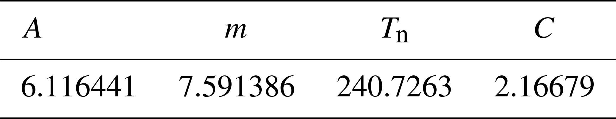
We computed the absolute humidity (in g m⁻³) according to Vaisala (2013) from the water vapour saturation pressure in the headspace of the prototype. Temperature and relative humidity are measured by the BME280 sensor.

$$\begin{array}{}\text{(C1)}& P_{\mathrm{WS}}=A\cdot {\mathrm{10}}^{\left(\frac{mT}{T+T_{\mathrm{n}}}\right)},\end{array}$$

where P_WS is the water vapour saturation pressure over water (in hPa) at temperature T (in °C), and A, m and T_n are given specific parameterisations for the temperature range of −20 to +50 °C (Table C1).

$$\begin{array}{}\text{(C2)}& P_{\mathrm{W}}=P_{\mathrm{WS}}\cdot {\displaystyle \frac{\mathrm{relH}}{\mathrm{100}}},\end{array}$$

where P_W is the dew point (in hPa) and relH is the relative humidity (in %). Absolute humidity, the mass of water vapour in a certain volume can be calculated assuming ideal gas behaviour:

$$\begin{array}{}\text{(C3)}& \mathrm{absH}={\displaystyle \frac{C}{T+\mathrm{273.15}}}\cdot {\displaystyle \frac{P_{\mathrm{W}}}{\mathrm{100}}},\end{array}$$

where absH is the absolute humidity (in g m⁻³) and C a constant (in gK J⁻¹) (Table C1).

Table C1 Parameters for the calculation of absolute humidity from Vaisala (2013).

Appendix D: Calculation of gas-specific Henry constants

The Henry constants for CH₄ and CO₂ (in mol L⁻¹ atm⁻¹) for freshwater are computed with the water temperature (T_W in kelvin) according to the equations reported in International Hydropower Association (2010):

$$\begin{array}{}\text{(D1)}& \begin{array}{rl}& {\mathrm{KH}}_{\mathrm{CH}\mathrm{4}}\left(T_{\mathrm{W}}\right)=\exp \left(-\mathrm{115.6477}+{\displaystyle \frac{\mathrm{155.5756}}{T_{\mathrm{W}}/\mathrm{100}}}\right.\\ & \left.+\mathrm{65.2553}\cdot \ln \left({\displaystyle \frac{T_{\mathrm{W}}}{\mathrm{100}}}\right)-\mathrm{6.1698}\cdot {\displaystyle \frac{T_{\mathrm{W}}}{\mathrm{100}}}\right)\cdot {\displaystyle \frac{\mathrm{1000}}{\mathrm{18.0153}}},\end{array}\end{array}$$

$$\begin{array}{}\text{(D2)}& \begin{array}{rl}& {\mathrm{KH}}_{\mathrm{CO}\mathrm{2}}\left(T_{\mathrm{W}}\right)=\exp \left(-\mathrm{58.0931}+\mathrm{90.5069}\right.\\ & \left.\cdot {\displaystyle \frac{\mathrm{100}}{T_{\mathrm{W}}}}+\mathrm{22.294}\cdot \ln \left({\displaystyle \frac{T_{\mathrm{W}}}{\mathrm{100}}}\right)\right).\end{array}\end{array}$$