Domain shifts in industrial condition monitoring: a comparative analysis of automated machine learning models

Selecting an appropriate model for industrial condition monitoring is challenging due to various factors. Typically, industrial datasets are small and lack statistical independence because experimental coverage of all possible operational variations is costly and sometimes practically impossible. Consequently, the resulting domain shifts pose a significant challenge. Although deep learning (DL) methods have frequently been regarded as the primary and optimal choice in many applications, they often lack major success factors in condition monitoring tasks. In this study, we benchmark the robustness of typical DL architectures against classical feature extraction and selection followed by classification (FESC) methods under domain shifts commonly encountered in industrial condition monitoring. Both DL and FESC methods are employed within an automated machine learning framework. We benchmarked these methods on seven publicly available datasets, and to simulate domain shifts, we employed leave-one-group-out validation on those datasets. Our experiments demonstrate high accuracy across all tested models for random K-fold cross-validation. However, the overall performance significantly decreases when faced with domain shifts, such as transferring the trained model from one machine to another. In four out of seven datasets, FESC methods showed better results in the presence of domain shifts. Furthermore, we also show that FESC methods are easier to interpret than DL methods. Finally, our results suggest that deep neural networks are not universally preferred over classical, low-capacity models for such tasks, as typically only a limited number of features from the input signal are needed.

1 Introduction

In industrial environments, mechanical systems undergo wear and tear, which can lead to faults and breakdowns necessitating maintenance. Maintenance plays a vital role in ensuring optimal functionality and prolonging the lifespan of these systems. Reactive maintenance, the traditional approach, involves responding to faults and failures as they arise, often resulting in prolonged periods of downtime. Conversely, preventive maintenance utilizes historical data to perform regular maintenance, aiming to prevent unforeseen failures; however, it includes unnecessary interruptions and services (Gertsbakh, 2000).

To overcome the limitations of these approaches, predictive maintenance and automated condition monitoring have emerged as a promising alternative. By applying advanced machine learning (ML) techniques, predictive maintenance analyzes data from various sensors and sources to detect patterns and trends that can be utilized for predicting future failures. Predictive maintenance minimizes downtime by identifying potential issues in advance or early stages, leading to substantial cost savings and improved efficiency (Mobley, 2002).

Industrial condition monitoring and predictive maintenance rely on the utilization of diverse sensors, such as pressure, vibration, and temperature sensors, to detect or predict approaching faults in industrial systems. Unlike computer vision tasks that involve extracting complex features from raw data (Olah et al., 2017), condition monitoring tasks typically rely on simpler statistical measures and a limited set of features (Schneider et al., 2018a). Traditionally, effectively dealing with industrial data requires domain experts' expertise and a feature engineering process to extract dependable features (Avci et al., 2021).

In recent years, there has been a noticeable shift in the field of condition monitoring, similar to the primary applications of ML, towards employing deep neural networks (DNNs) for direct analysis of raw data, bypassing the traditional feature engineering process (Zhao et al., 2019). Although this approach has shown promising results, it is not without its challenges. The inherent complexity of DNN models makes optimization of their hyperparameters (HPs) difficult, presenting a significant challenge. Additionally, the interpretability of DNN decisions remains an unresolved issue (Selvaraju et al., 2020). Alternatively, the adoption of automated machine learning (AutoML) techniques offers a viable solution. AutoML is an advanced methodology that automates various aspects of ML, including feature engineering, model selection, and HP optimization. Its primary goal is to enhance the accessibility of ML for non-experts by reducing the need for manual intervention in model development (Truong et al., 2019). AutoML algorithms can automatically explore a predefined set of models and associated HPs or even perform neural architecture searches to discover novel model architectures that deliver optimal performance for a given task (He et al., 2021). By leveraging these algorithms, users can smooth the ML process and obtain high-performing models without extensive manual experimentation.

In supervised ML, a common assumption is that both the training data and test data are drawn independently and identically from the same distribution. However, this assumption may not always hold in practical scenarios like condition monitoring and predictive maintenance, where the presence of various operational conditions can cause covariate shifts in the data distribution. These operating conditions, such as temperature variations, changes in rotational speed, load variations, pressure fluctuations, or substituting the target machine with another, can have a significant impact on the performance and generalization of ML models (Goodarzi et al., 2022). As a result, it becomes crucial to address domain shift challenges to ensure the effectiveness and reliability of the predictive models in real-world critical applications.

In this research, an experimental approach is employed to compare the performance of AutoML methods for condition monitoring and predictive maintenance applications. Our AutoML framework includes classical feature extraction, feature selection, and classification (FESC) methods, as well as DNN solutions with automatic HP optimization. While existing studies have focused on comparing and benchmarking ML methods for fault detection in time series signals, our work distinguishes itself by taking a more comprehensive approach, utilizing real-world practical datasets and considering domain shift problems. Pandarakone et al. (2019) examined the effectiveness of classical ML classifiers and convolutional neural networks (ConvNets) in detecting bearing faults in induction motors. Buckley et al. (2022) conducted experiments on benchmark feature extraction (FE) and feature selection (FS) methods for structural health monitoring using two datasets. Fawaz et al. (2019) explored various methods, including deep learning models, for time series analysis on UCR (University of California, Riverside) and UEA (University of East Anglia) (Dau et al., 2018) datasets. Data augmentation (Wen et al., 2021) is a technique used to expand the training data and introduce variation to the dataset, enhancing the model's robustness against potential changes in test data. Implementing data augmentation requires domain knowledge to ensure that the transformations are meaningful and do not alter the labels. In industrial applications, data are often complex and challenging to interpret, requiring expert input to tailor appropriate and effective augmentation strategies for each specific dataset and use case.

In this study, we carefully selected diverse datasets from the industrial condition monitoring field, varying in both size and use case. Specifically, they are sourced from sensors in a time series format, consisting of one-dimensional data. Moreover, different validation strategies are employed in our study. Through the comparison of these strategies, we aim to examine the impact of domain shift (Goodarzi et al., 2022) on the performance of various ML methods.

This paper contributes by comprehensively evaluating various ML methods using openly accessible data and addressing domain shift issues. We assess the performance of these methods across different datasets and discuss their relative strengths and limitations in condition monitoring and predictive maintenance use cases. In this work, HP optimization and model selection are integral parts of our AutoML framework in realistic real-world application scenarios.

2 Datasets and validation scenarios

In this study, we analyzed various publicly available datasets in condition monitoring and predictive maintenance. Our selection included datasets of different sizes and numbers of observations, ranging from simple to large-scale use cases. The primary focus of this article is on supervised learning tasks with predetermined target values. Although certain tasks may involve regression, our primary focus in this study is on the classification format of these tasks. Furthermore, to minimize additional HPs and complexities associated with multi-modality, only a single sensor was selected from each multi-sensor dataset for the initial analysis. Extending the methods to fully utilize multi-sensor datasets is a direction we plan to explore in future work.

2.1 Validation scenarios

Conventional random K-fold cross-validation typically assumes that both training and validation subsets are drawn from the same distribution. To highlight potential distribution shifts within these datasets, we employed leave-one-group-out (LOGO) cross-validation tailored to each dataset's specifications or working conditions. Utilizing LOGO validation under carefully chosen cross-influence conditions provides a valuable measure for assessing the model's ability to generalize to unseen domains (Gulrajani and Lopez-Paz, 2020). Condition monitoring datasets are typically the result of carefully designed experiments that control working conditions and can be leveraged for selecting validation groups. In addition to prior knowledge about the possible underlying data distributions used to define these groups, several methods exist to discover meaningful data subsets automatically (Singla et al., 2021; d'Eon et al., 2022; Atanov et al., 2022). Automated approaches utilize learned models to identify slices of data where model performance is suboptimal.

We compared the results of expert-specified LOGO cross-validation with random K-fold cross-validation to highlight the challenges that domain shift poses for model selection. To maintain consistency in the experiments, we used stratified resampling and ensured that the number of folds in the K-fold scenario matched the number of distinct groups in the LOGO validation scenario for a fair comparison. Below is an overview of the datasets employed in this study.

2.2 The Case Western Reserve University (CWRU) bearings

The CWRU dataset (CWRU Bearing Data Center, 2019) is widely recognized in the field of predictive maintenance and has been extensively utilized in numerous studies. The primary objective of this dataset is to perform a binary classification task, specifically distinguishing between various fault types and healthy devices. The classes in the dataset include “healthy”,” “inner ring” faults, “outer ring” faults, and “ball” faults.

The data comprise vibration signals obtained from bearings experiencing different fault types and varying load conditions. The recordings are specifically collected for different motor loads, namely 0, 1, 2, and 3 HPs that are used for LOGO validation. To ensure consistency, the recordings in the dataset are sampled at a rate of 12 kHz, and the data are segmented into non-overlapping slices of 1 k length.

2.3 The ZeMA hydraulic system (HS)

The HS dataset (Schneider et al., 2018b) comprises recordings from a test bed equipped with multiple sensors (17) capturing data under various fault conditions. The target variable in this dataset is the accumulator pre-charge pressure. For LOGO validation, the cooler performance at 3 %, 20 %, and 100 % is regarded as the crucial control variable.

In this dataset, the analysis focuses solely on recordings from the first pressure sensor (PS1). Two system variables, namely the valve state and the accumulator (Acm) state, are selected as the target variables. As a result, the dataset is split into two versions for this study, namely HS (valve) and HS (Acm).

2.4 ZeMA electromechanical axis (EA)

The dataset (Klein, 2018) consists of data collected from 11 sensors during the lifetime measurement of the axis. The electromechanical axis follows a fixed working cycle of 2.8 s, including a forward stroke, waiting time, and a return stroke. For dataset creation, 1 s of the return stroke from every 100th working cycle was selected. In this dataset, the target variable is divided into five categories, ranging from 1 representing a new device to 5 representing a near-failure device. This classification task is utilized for lifetime estimation.

The dataset specifically utilizes the microphone as the input sensor, with a sampling rate of 2 kHz. In the LOGO validation scenario, the performance of the models is evaluated using four different devices. This approach helps assess the generalizability and robustness of the models across various devices.

2.5 Open guided wave (OGW)

The OGW dataset (Moll et al., 2019a) consists of time series signals that capture guided waves recorded at various temperature levels, ranging from 20 to 60 °C with 0.5 °C increments. The signals were collected using 12 ultrasonic transducers arranged in a sender–receiver configuration. These transducers were attached to a carbon-fiber-reinforced polymer (CFRP) plate, which had a detachable aluminum mass positioned at four different locations to simulate delamination damage.

To generate the signals, a five-cycle Hann-windowed sine wave was used as the source signal, with frequencies varying from 40 to 260 kHz in 20 kHz increments. The measurements were initially conducted on an intact CFRP plate at different temperature levels. Subsequently, the measurements were repeated with simulated damage at each of the four positions, along with measurements of the intact plate. These four locations of simulated damage were used for the LOGO validation scenario. The objective of this use case is to detect whether the CFRP plate is damaged or intact, thereby presenting a binary classification task.

2.6 Paderborn University (PU) bearing

The PU dataset (Lessmeier et al., 2016) is a well-known and frequently utilized dataset in the field of bearing analysis. It comprises recordings of high-frequency vibrations and motor currents from a total of 32 bearings, consisting of 26 faulty bearings and 6 healthy bearings.

In addition to the vibration and current data, the dataset provides measurements of speed, load, torque, and temperature, offering comprehensive information for analysis. The signals were collected under four different working conditions, each representing a distinct operating scenario. These working conditions are used for the LOGO cross-validation strategy in this study.

2.7 Naphthalene concentration (Naph)

The Naph dataset (Bastuck et al., 2015) consists of recordings from a gas sensor operating at different temperatures. The sensor signals were sampled at a rate of 4 Hz. The dataset focuses on the detection and analysis of naphthalene concentrations in the presence of ethanol as a background or interfering gas. Indeed, despite the dataset not being originally from the condition monitoring domain, it exhibits similarities with datasets used in condition monitoring, particularly in terms of signal shape and cross-influence variables. These similarities make it feasible to employ a meaningful LOGO validation approach for the study.

The dataset includes measurements of six different concentrations of naphthalene. These concentrations were repeated for three levels of ethanol, representing different interference scenarios. The dataset is designed to evaluate the sensor's performance in detecting and quantifying naphthalene concentrations accurately in the presence of varying ethanol levels. To evaluate the performance of algorithms and models, the dataset employs the LOGO cross-validation strategy using the ethanol concentrations as distinct groups.

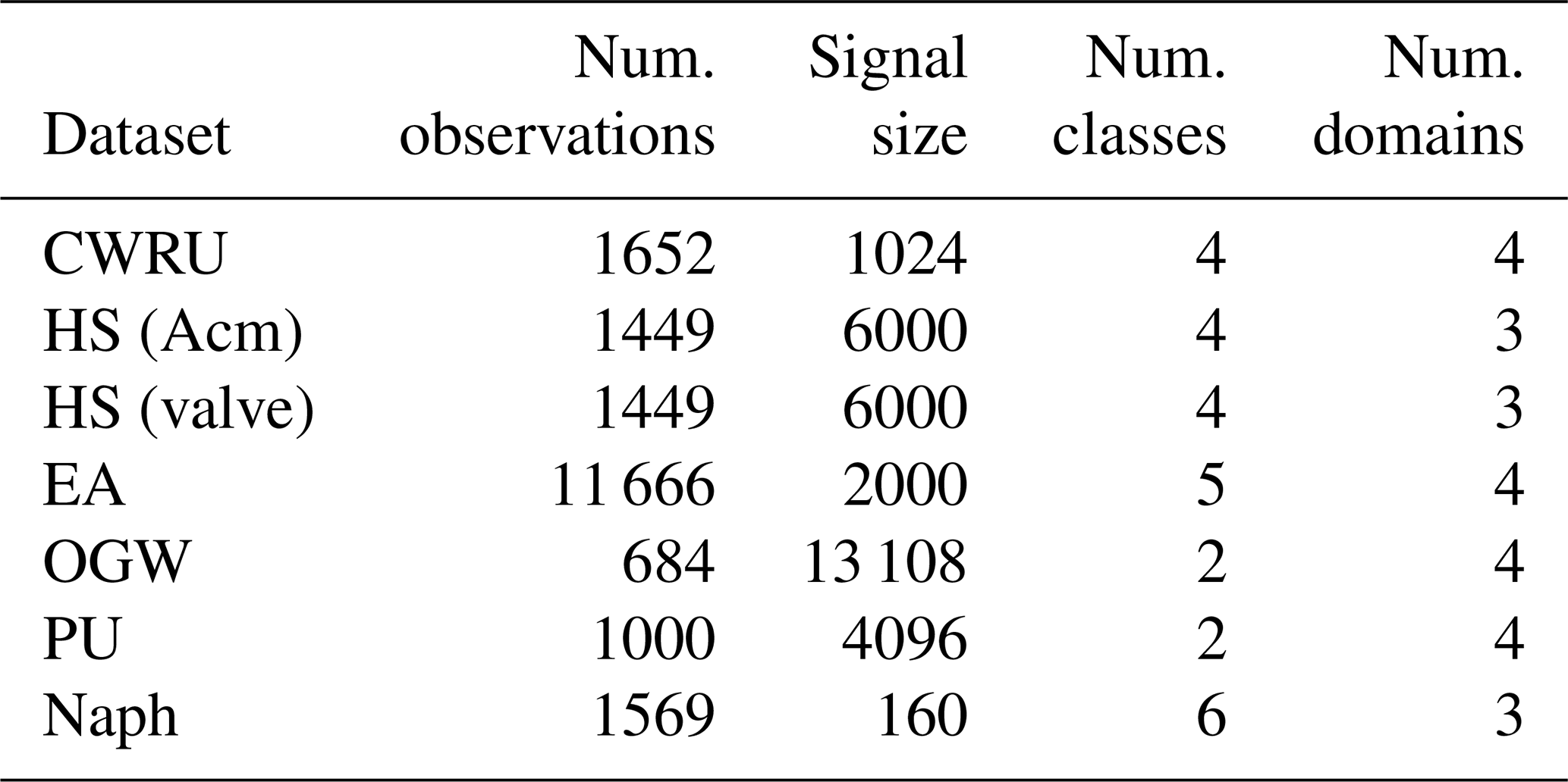
Table 1 provides a summary of the dataset's features. The datasets share common characteristics, typically consisting of fewer than a few thousand observations, and the number of classes is relatively limited, with most having fewer than six classes. However, the data size can vary significantly, ranging from 100 to 10 000 data points. To maintain consistency across all scenarios, we used balanced versions of the datasets, ensuring that the number of observations from each class is approximately equal.

Table 1 Overview of study scenarios.

3 Methods

3.1 FESC methods

The training, evaluation, and model selection of the FESC methods are performed using a MATLAB-based (The MathWorks Inc., 2022) AutoML framework (Schneider et al., 2018a). The framework employs an exhaustive search strategy to determine the best combination of FE, FS, and classification methods. The methods are listed in Table 2.

(Olszewski et al., 2001)(Goodarzi et al., 2023)(Wold et al., 1987)(Schneider et al., 2018a)(Kirch, 2008)(Kononenko et al., 1997)(Lin et al., 2012)(Spearman, 1904)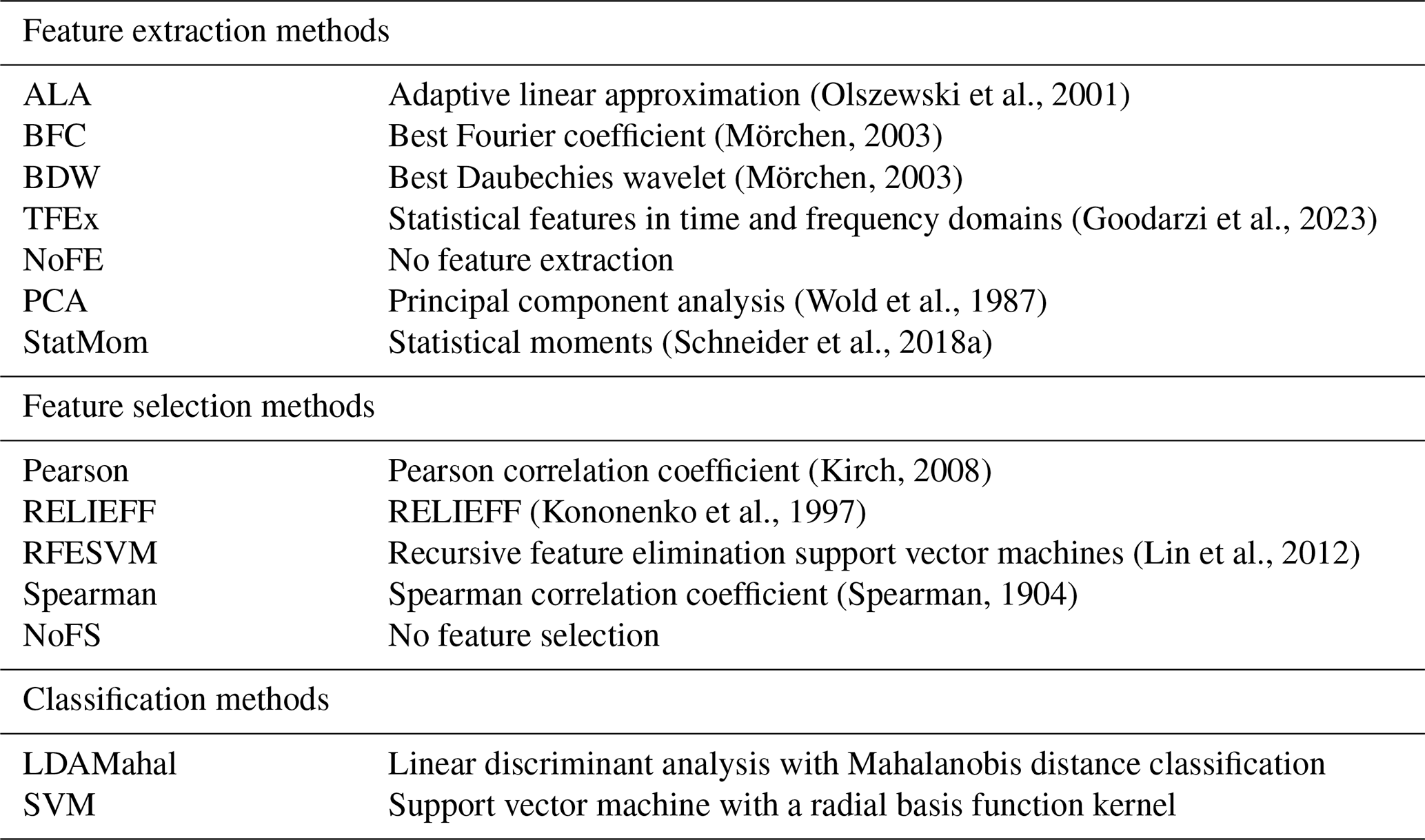

Table 2 FESC methods implemented in the AutoML framework.

The automated FESC method used in this study has demonstrated impressive performance, as documented in multiple previous studies (Schneider et al., 2018a; Goodarzi et al., 2023; Schnur et al., 2022). Its usage in this investigation is motivated not only by its performance but also by its focus on the interpretability and explainability of the models (Goodarzi et al., 2022). In industrial ML applications, model interpretability is a vital factor in ensuring the acceptance and validation of the model by domain experts (Hong et al., 2020).

In our FESC framework, a variety of FE methods are employed to cover both the time and frequency domains. Specifically, three methods, adaptive linear approximation (ALA) (Olszewski et al., 2001), principal component analysis (PCA) (Wold et al., 1987), and statistical moment (StatMom) (Schneider et al., 2018a), are used to extract features from the time domain, each using distinct approaches to tackle different use cases. In contrast, the best Fourier coefficient (BFC) (Mörchen, 2003) focuses on the frequency domain for FE. The best Daubechies wavelet (BDW) (Mörchen, 2003) and statistical features in time and frequency domains (TFEx) (Goodarzi et al., 2023) extract features from both time and frequency domains. Additionally, a “no-feature extraction” (NoFE) approach is employed, which essentially does not alter the data. This approach can be beneficial when working with data instances of limited duration or when the raw data already contain the necessary information for classification. The collection of FE methods enables the exploration of different feature representations for each classification task. The complete evaluation using FESC involves testing 70 (7 FE methods × 5 FS methods × 2 classification algorithms) combinations of methods for the desired tasks.

3.2 Deep learning methods

To represent the deep learning methods, we explore four neural network architectures: multi-layer perceptron (MLP) (Haykin, 1994), ConvNet (Schmidhuber, 2015), residual network (ResNet) (He et al., 2016), and WaveNet (Oord et al., 2016). To achieve optimal network configurations, each architecture is subjected to HP optimization. The specific parameters utilized for optimizing each network are outlined in Table 3. Through this comprehensive evaluation, we aim to identify the most suitable neural network architecture for the given tasks.

Table 3 Ranges of hyperparameters for various DNN architectures.

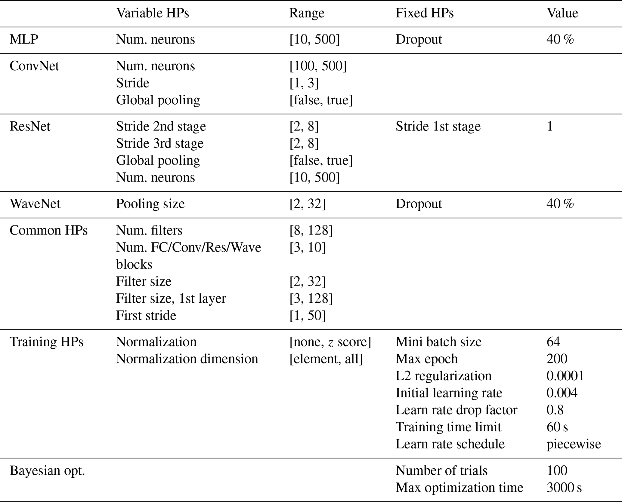
Training neural networks can be computationally expensive, especially when combined with the challenge of HP optimization. To address this, early stopping and Bayesian optimization are employed to reduce the computational load. The maximum number of iterations for Bayesian optimization is set to 100, with a maximum time limit of 3600 s. In this study, we adopt Adam optimization as the optimization method for all networks, while employing the cross-entropy loss function for the training process.

The training process is conducted using Nvidia RTX 5000 GPUs, with a maximum mini-batch size of 64 to accommodate hardware limitations.

3.2.1 Multi-layer perceptron

The architecture of the MLP network comprises multiple blocks, with each block containing a sequence of layers including a fully connected layer, a batch normalization layer, and a ReLU (rectified linear unit) activation layer. Figure 1a provides a visual representation of the structure of the MLP network, showcasing the arrangement of its components within each block. The MLP architecture has been widely employed in various condition monitoring applications (Avci et al., 2021; Fawaz et al., 2019), highlighting its relevance and applicability in the field. In our MLP network design, the quantity of neurons within each block adheres to the following mathematical expression:

$$\begin{array}{}\text{(1)}& N\left(i\right)=N_{\mathrm{b}}/(\mathrm{2}i-\mathrm{1}).\end{array}$$

In this equation, we use i to signify the block number, while N denotes the count of neurons, and N_b stands for the initial neuron count. It is important to note that the architecture of the network is shaped by two fundamental factors: the number of blocks and the initial neuron count, which is represented as N_b.

Figure 1 Structure of MLP (a) and ConvNet networks (b).

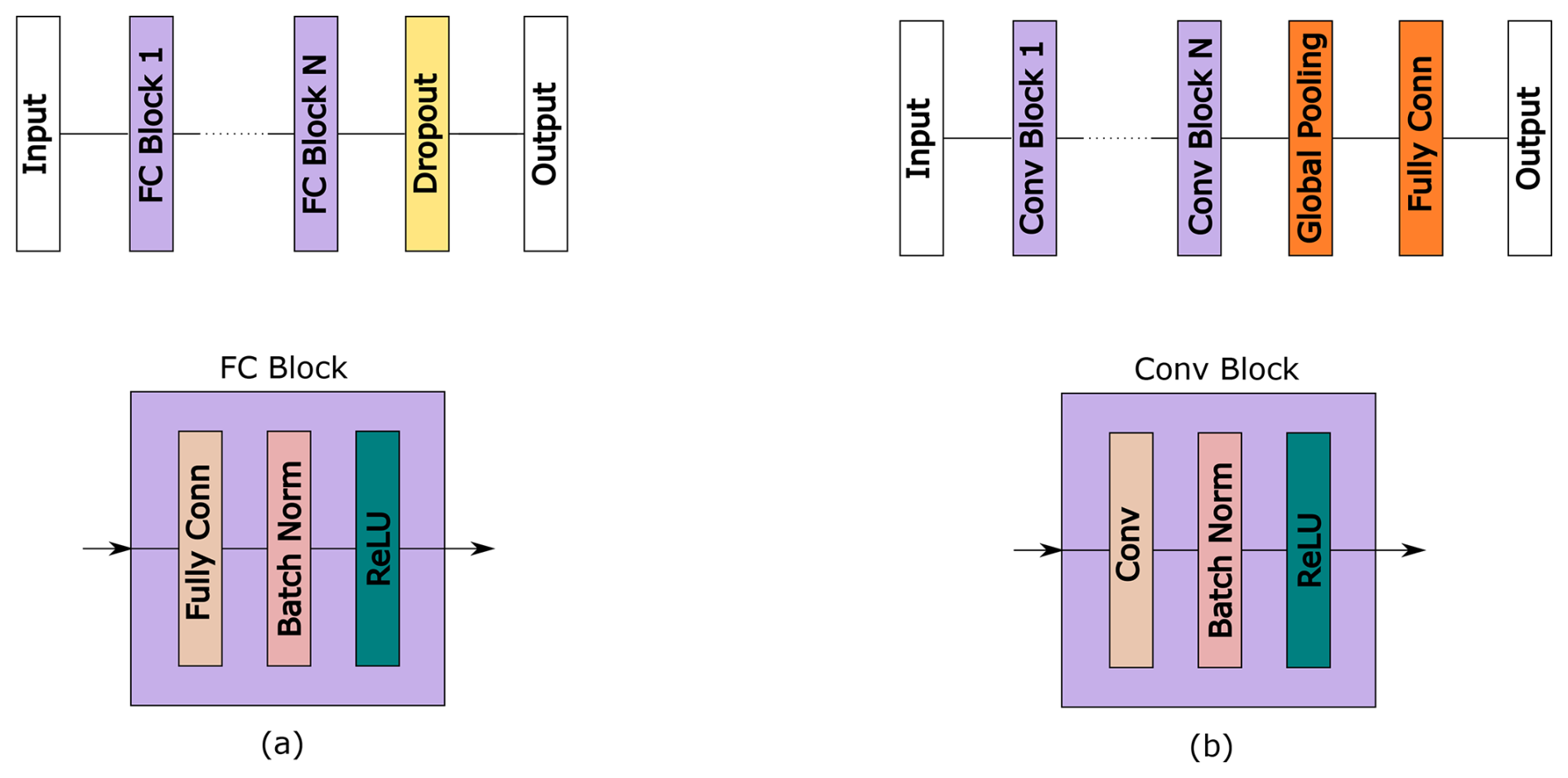
To prevent overfitting, we include a dropout layer at the end of the network, which randomly drops out some neurons during training. Notably, the number of neurons in each block decreases as the depth of the network increases. This progressive shrinking of the number of neurons in deeper layers helps reduce the overall complexity of the model, mitigating the risk of overfitting and enhancing the generalization performance.

3.2.2 Convolutional neural network

The ConvNet architecture in this study consists of multiple convolutional blocks, each designed to extract features from the input data (Fig. 1b). The first block has its own filter size and stride, which are independent of the subsequent blocks. However, all the remaining blocks share the same filter and stride size. The number of filters within each convolutional block is calculated by doubling the initial filter count for each block, as indicated by the following equation:

$$\begin{array}{}\text{(2)}& N_{\mathrm{f}}\left(i\right)=N_{\mathrm{fb}}\times {\mathrm{2}}^{i-\mathrm{1}}.\end{array}$$

In this equation, N_f represents the filter count in the ConvNet block, N_fb is the initial filter count, and i signifies the ConvNet block number. Once the convolutional layers have processed the input, we apply global pooling to aggregate the output of each feature map into a single value. The purpose of the fully connected layer is to perform classification based on the learned features.

The ConvNet architecture is a popular choice for image classification tasks due to its ability to capture spatial relationships and extract relevant features from input images through convolutional layers. It is also commonly used in time series classification (Avci et al., 2021; Fawaz et al., 2019; Kiranyaz et al., 2021). As the number of filters in each block increases, the network learns more complex and abstract features when going deeper. The global pooling layer helps reduce the number of parameters in the fully connected layer, making the model more efficient and reducing the risk of overfitting. Furthermore, the inclusion of dropouts during training helps to mitigate the overfitting problem by introducing randomness during training.

3.2.3 Residual network

Deep neural networks often face the challenge of the vanishing gradient problem, which can affect their performance. To overcome this issue, the ResNet architecture introduces skip connections. These connections enable gradients to bypass several intermediate layers. This method not only helps to mitigate the vanishing gradient problem but also combines features from different depths, resulting in effective detection of intricate patterns.

The ResNet architecture consists of multiple blocks, each containing convolutional layers, batch normalization, and ReLU activation functions, as shown in Fig. 2. The first block of the network has a larger filter and stride size. A larger filter size helps in capturing abstract features and mitigating input noise, while a larger stride size reduces the spatial dimensions of the input by downsampling. The subsequent blocks within the same stage use the same filter and stride sizes to preserve the feature map dimensions in a deep network.

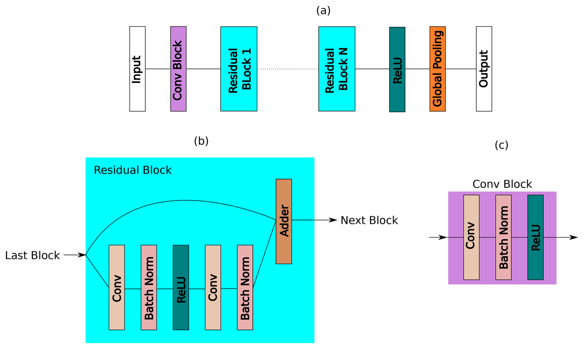
Figure 2 Structure of ResNet. (a) The main structure, (b) the residual block, and (c) the convolutional block.

ResNet uses skip connections to help the network learn residual mappings, which model the difference between the desired output and the input. This residual is added back to the layer's input to obtain the final output, enabling the network to learn deeper and more descriptive representations. As demonstrated by Fawaz et al. (2019), this approach improves performance on challenging tasks.

The number of filters (N_f) in each block is determined by Eq. (2); however, in this case i is the stage number. The overall number of blocks (N_Bl) is divided into stages, with each stage comprising a set number of blocks (N_s). This number of blocks per stage, denoted as N_s, is calculated as follows:

$$\begin{array}{}\text{(3)}& N_{\mathrm{s}}=\text{floor}(N_{\mathrm{Bl}}/\mathrm{3}).\end{array}$$

Here, we use the “floor” function to obtain the largest whole number less than or equal to the result of dividing N_Bl by 3.

3.2.4 WaveNet

The WaveNet architecture (Oord et al., 2016), originally developed by Google for audio generation, has demonstrated its effectiveness in various domains including speech recognition, music synthesis, and vibration signal classification (Zhuang et al., 2019). WaveNet incorporates two distinctive characteristics that contribute to its success.

One of the key strengths of WaveNet is its use of dilated convolutions. This technique allows the model to capture long-term dependencies in the data by applying convolutional filters with exponentially increasing dilation factors. By expanding its receptive field, WaveNet can effectively detect patterns across a larger context. This is particularly useful when dealing with long signals, as it helps the network to capture important information from a wider range of data.

The second feature of WaveNet is the inclusion of skip connections, which are similar to the ResNet architecture. These skip connections facilitate the direct transmission of information between layers, mitigating the loss of information as the network grows deeper. By preserving and propagating relevant information, skip connections enhance the model's ability to learn complex representations and facilitate the training of deep architectures.

The current study defines a parametric WaveNet architecture by using essential parameters such as the number of blocks, filter length, stride of the initial block, filter size, number of filters in each subsequent block, and pooling size of the final stage, as depicted in Fig. 3. The dilation factor follows an exponential growth pattern, which is similar to the one outlined in the original WaveNet paper.

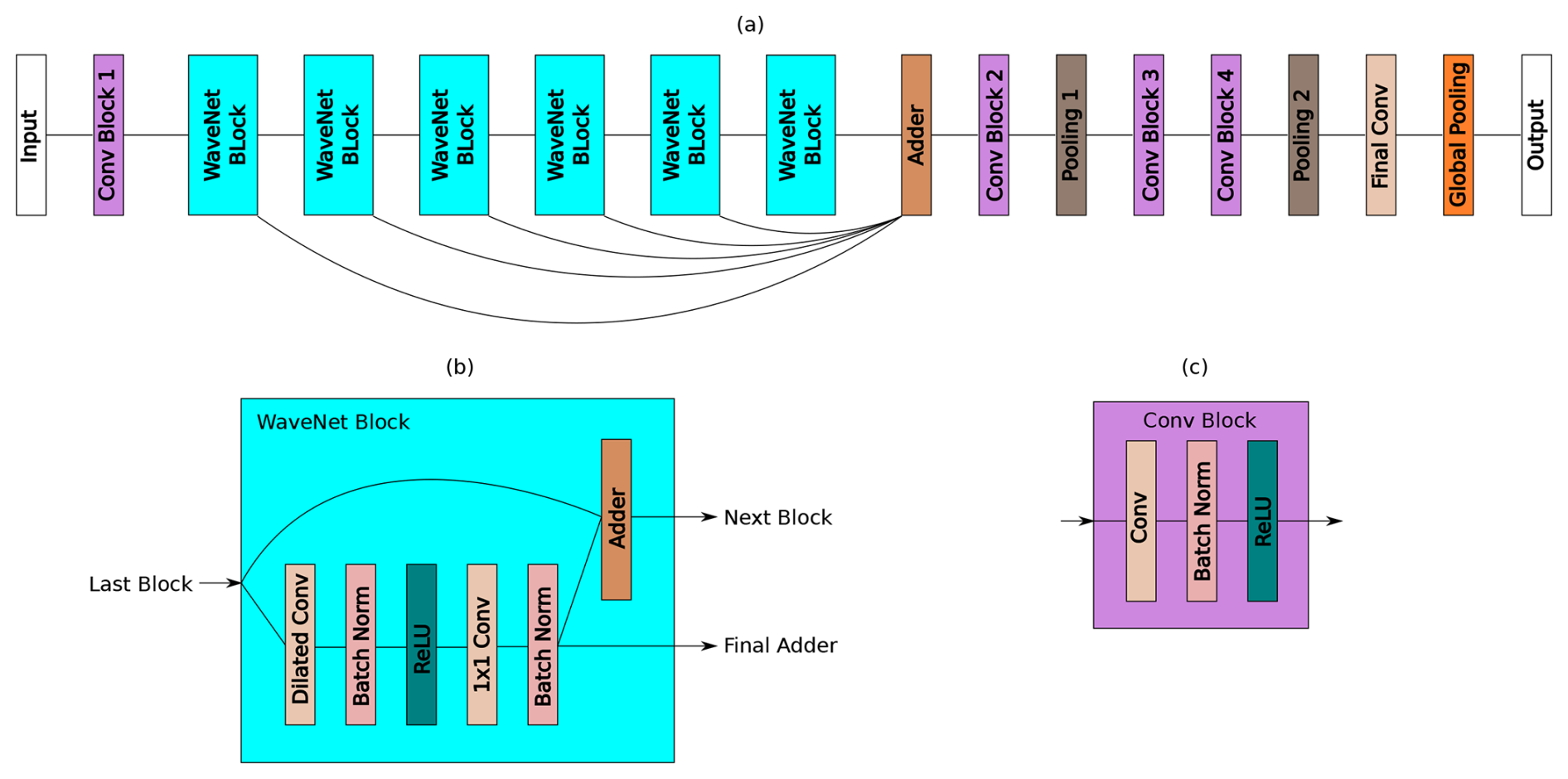
Figure 3 Structure of WaveNet. (a) The main structure, (b) the WaveNet block, and (c) the convolutional block.

3.3 Evaluation and model selection

We evaluated the performance of the models using accuracy as the metric. Accuracy is a commonly used metric in classification tasks. It is calculated by dividing the number of correct predictions by the total number of observations. It indicates how well the models can classify the data correctly. It is most useful when dealing with balanced datasets, as it provides an overall measure of the correctness of the model's predictions. Alternatively, accuracy (acc) can be expressed as 1 minus the error rate (err). The error rate is the expected value of the 0-1 loss across all observations, which is the loss when a prediction does not match the true label.

$$\begin{array}{}\text{(4)}& {\displaystyle }\mathrm{err}={\displaystyle \frac{\mathrm{1}}{n}}\sum _{i=\mathrm{1}}^n\left[y_i\ne f\left(x_i\right)\right]\text{(5)}& {\displaystyle }\mathrm{acc}=\mathrm{1}-\mathrm{err}\end{array}$$

3.4 Occlusion map

Deep learning models are often considered black boxes due to their lack of interpretability and explainability. However, in situations where it is necessary to explain the model's decisions, saliency maps can be a helpful tool to provide an explanation and cover this weakness. One such saliency method is the occlusion map, which works by applying the occlusion technique to different parts of the input and measuring the network's sensitivity to these changes. This helps to create an attribution map that highlights the crucial regions of the input that contribute to the decision-making process. It is important to note that the occlusion map is a local attribution method, meaning that it explains the model's decisions regarding a specific input and not the general function of the model.

To effectively perform occlusion mapping, three key parameters need to be carefully defined. The first parameter is the mask size, which determines the size of the sliding window used to occlude different regions of the input. The second parameter is the stride size, which determines the step size for sliding the mask over the input. Finally, the mask value is the value that replaces the original input value during the perturbation process.

Overall, occlusion maps provide an intuitive and easily interpretable approach to understanding the decisions made by neural networks where interpretability is important, such as critical industrial tasks.

4 Results

This section presents the evaluation results of both FESC and DNN methods across the tested datasets. The findings begin with benchmark comparisons and proceed to an exploration of feature selection and the interpretability of the methods.

The bar graph in Fig. 4 illustrates the accuracies of the evaluated models, categorized into two validation strategies: LOGO and K-fold. For the majority of use cases (five out of seven), all models demonstrate near-perfect accuracy under K-fold validation, making it challenging to distinguish performance differences among them. Conversely, LOGO validation reveals a different trend, with near-perfect accuracy achieved by only a limited number of models in two specific use cases: CWRU and HS (valve). FESC methods achieve the highest accuracy in HS and OGW or rank as a close runner-up with only a marginal difference in CWRU, PU, and Naph. LOGO validation results on the EA dataset reveal the most significant performance drop across all methods, with accuracies dropping to nearly random guessing. This underscores the severe generalization challenges arising when models are applied across different devices.

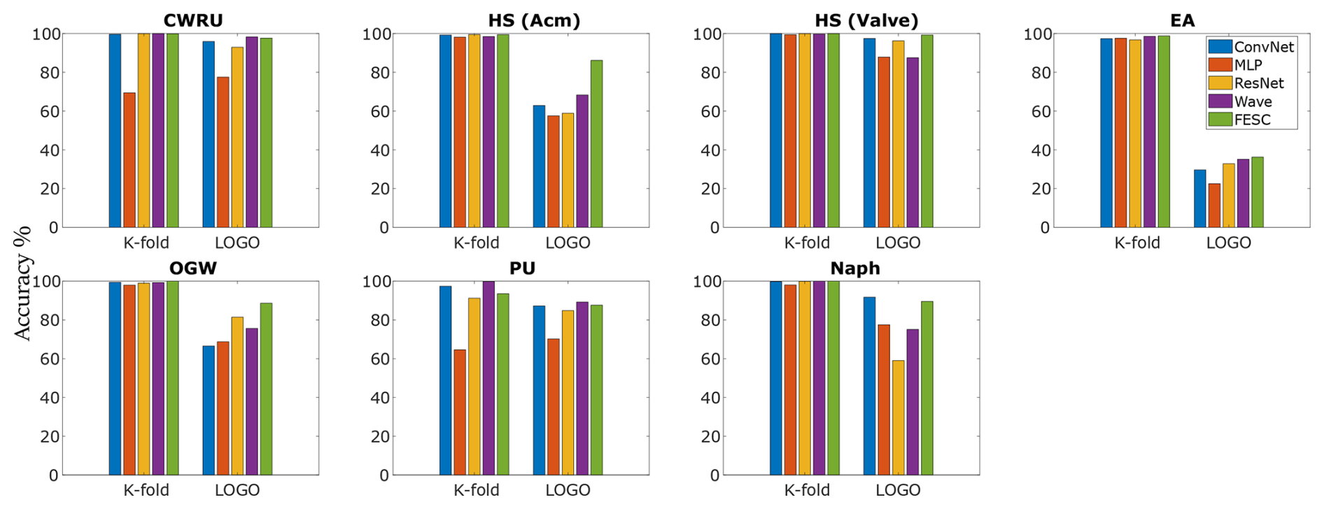
Figure 4 Comparing the accuracy of various networks and FESC methods in both K-fold and LOGO scenarios.

Figure 4 only shows the accuracy of the best FESC model; however, our framework explores a variety of models for each task. The box plots of cross-validation errors from the models are shown in Fig. 5. Consistent with previous findings, LOGO validation scenarios consistently result in higher error rates compared to K-fold validation. Furthermore, the errors in LOGO validation exhibit greater variability across datasets, with the exception of CWRU and PU, where the variations in both cases are comparable. Notably, for the HS (Acm and valve) datasets, the tested models achieved high accuracies under LOGO validation of 85 % and 97 %, respectively. However, there was a significant difference of approximately 60 % between the best and worst accuracies for the datasets. Figure 5b provides a histogram of the selected features of the top three FESC methods for each scenario, revealing that 44 % of the top models use fewer than 20 features of the input signal after feature selection.

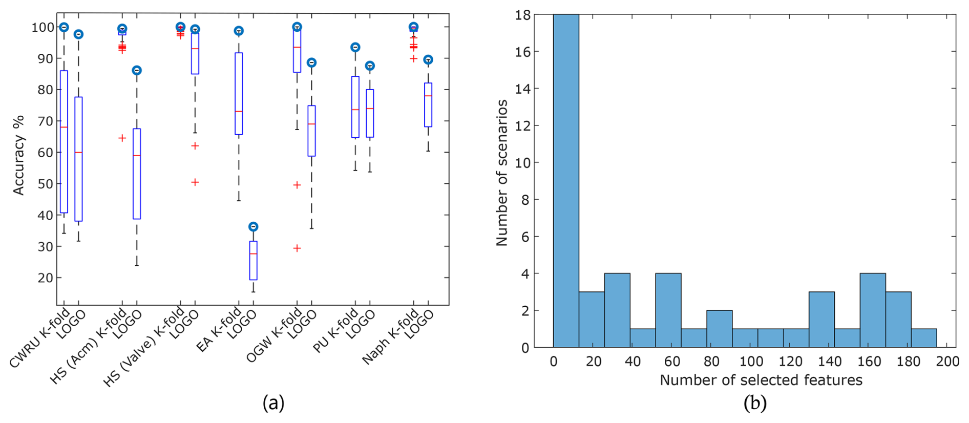
Figure 5 (a) A visual comparison of box plots, depicting the errors of conventional models from the FESC methods in both LOGO and K-fold validation scenarios. For each task, the model with the highest cross-validation accuracy is indicated by the circles. (b) Histogram depicting the distribution of the number of selected features for the top three FESC models.

The remainder of this section provides a comparative analysis of the interpretability of results obtained from FESC and DNN methods. As a case study, we focus on the HS (valve) dataset under LOGO validation. To evaluate the results, we leverage expert knowledge of the task. Among the observed signal variations, only the first drop in the signal (depicted in Fig. 6) is attributed to the valve's operation, whereas the subsequent steps are related to the designed process. For comparison, we selected the models with the highest accuracy from both method groups.

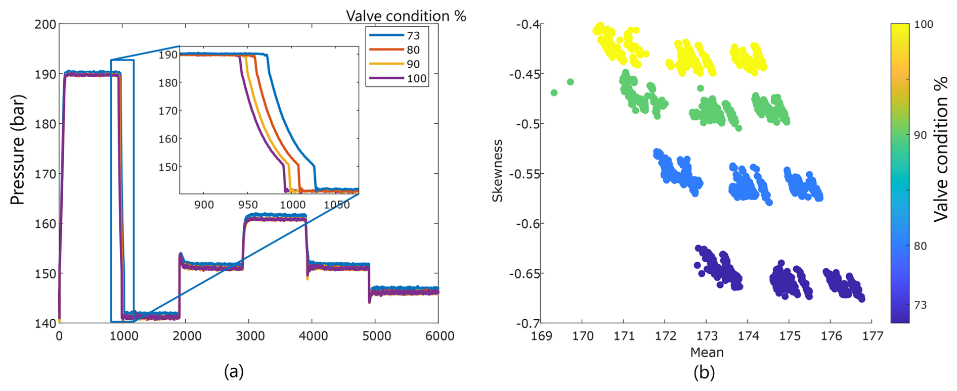
Figure 6 (a) Four representative observations from the HS (valve) dataset. (b) Key features identified by the best model as the most important.

The FESC model achieving the highest accuracy comprises statistical moments as the FE method, Pearson correlation as the feature selection FS method, and SVM as the classifier. During the classification step, only four features from the extracted set were employed. By mapping these features back to the raw signal, it becomes possible to identify the critical regions of the signal, particularly the switching region of the valve. A clear visualization of the effectiveness of two selected features is presented in Fig. 6b, illustrating three distinct clusters corresponding to each class label. These clusters represent the cooler performance in the LOGO validation scenario.

Explaining the decisions made by DNNs poses a significant challenge, leading to the development of various methods to interpret their predictions. One such method is the use of occlusion maps, which visualize the critical regions in the input data that influence model decisions. For the HS (valve) dataset, the ConvNet model achieved the best results, and we leveraged prior knowledge from classical methods to guide the interpretation of its attributions. Since true labels for the attributions were unavailable, a grid search was conducted to optimize the HPs of the occlusion maps.

We imposed constraints on the parameters to enhance feature identification accuracy. Specifically, the mask size was restricted to a maximum of 1000 to prevent the overlap of two transactions of the signal. At the same time, a smaller mask size was preferred to pinpoint critical features effectively. The grid search spanned mask sizes and strides ranging from 5 to 1000 to identify optimal parameter values. Figure 7 presents the attribution maps of observations with 100 % cooling performance for three sample mask sizes and four stride sizes. Although the peak position and magnitude in the attribution maps vary with parameter selection, the network consistently highlights a similar region in the input data as the most influential feature.

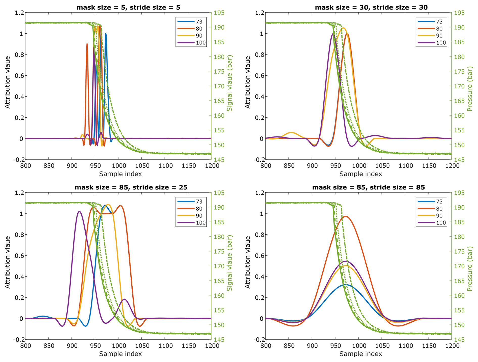
Figure 7 Four different combinations of mask size and stride settings for generating occlusion maps.

5 Discussion

The findings of this study highlight the critical importance of adopting realistic validation scenarios to ensure robust model performance in the presence of domain shifts.

Figure 4 highlights the clear differences in accuracy between methods under the two validation strategies. Additionally, Fig. 5a illustrates that the variation in performance between methods is significantly higher with LOGO validation. This underscores the challenges posed by domain shift, a common issue in real-world scenarios where data distributions often differ between training and application environments. FESC methods consistently outperform other approaches on most tested datasets under LOGO validation, striking an effective balance between model complexity and generalization, as described by the bias–variance trade-off (Hastie et al., 2009).

While no definitive winner emerges among the DNN architectures based on Fig. 4, it is evident that for datasets involving vibration signals (CWRU, PU), the MLP network consistently exhibited the lowest overall mean accuracy. This highlights its limitations in effectively capturing the underlying patterns in dynamic data. In contrast, ConvNet achieved the highest overall accuracy among the tested networks. Notably, other studies have shown that ResNet, a more advanced ConvNet architecture, outperforms simpler ConvNet models as the number of layers increases, enhancing its ability to learn complex patterns. The observed differences in performance may also be influenced by the hyperparameter optimization process and its specific variations across these networks. Among all architectures, WaveNet demonstrated superior performance for the two vibration datasets, aligning with its design strengths, such as handling long input signals and utilizing receptive fields of varying sizes. These features make WaveNet particularly effective in extracting meaningful characteristics from vibration data.

In most supervised machine learning tasks related to condition monitoring, the number of target classes is typically limited and often reducible to just two: healthy and faulty cases. This stands in obvious contrast to datasets like AudioSet (Gemmeke et al., 2017), which contains over 500 classes, or the well-known ImageNet (Deng et al., 2009), with 1000 classes. Given the constrained number of observations, target classes, and required features, low-capacity models are generally sufficient to achieve effective performance. This phenomenon is evident in Fig. 5b, where 44 % of the top-performing models achieve high accuracy using fewer than 20 features from the input signal, aligning with the well-documented curse of dimensionality (Bellman, 1961).

As mentioned in the Results section, the FESC methods of the AutoML framework offer a significant advantage in terms of interpretability. These methods are structured as separate blocks, each serving specific functions, which facilitates the identification of crucial features. This interpretability is particularly enhanced when a limited number of features are used, and linear methods are employed. However, precisely identifying the specific features within that highlighted region remains a challenge and requires further investigation.

In the remainder of this section, we explore additional differences between DNN models and the FESC approach, starting with HP optimization. HP optimization is a critical yet resource-intensive phase in model development, demanding significant time and computational resources. As outlined in Sect. 2, we meticulously optimized the HPs of the neural networks over an extensive range of parameters. In contrast, the FESC methods did not undergo explicit HP optimization; the only parameter adjusted during cross-validation was the optimal number of features, determined after feature selection. Consistent with the presented results, this highlights the substantial number of HPs that must be addressed when employing DNNs, emphasizing the complexity and computational demands of these models compared to the FESC approach.

A final consideration in comparing DNNs and FESC methods lies in their scalability with respect to the number of observations and classes. Certain FESC methods, such as one-vs.-one SVM, face scalability challenges, as their training time grows quadratically with the number of classes due to the need for $N(N-\mathrm{1})/\mathrm{2}$ binary classifiers for N classes. Conversely, DNNs, with their reliance on backpropagation and specialized frameworks optimized for high-end GPUs, can efficiently manage large datasets with numerous observations and classes. However, in the context of condition monitoring applications – characterized by limited observations, target classes, and necessary features – these scalability advantages of DNNs are less critical. Instead, FESC methods remain viable and computationally efficient, emphasizing their continued relevance in such domains.

Although the primary focus of this study is on industrial data and condition monitoring tasks, the methods presented are applicable to other domains with similar data types. Examples include human activity recognition using vibrational and accelerometer sensors (Reyes-Ortiz et al., 2015).

6 Conclusions

In conclusion, this research provides a comprehensive study comparing AutoML approaches utilizing FESC methods and DNN models for industrial condition monitoring tasks.

The experimental results reveal several significant insights. Firstly, random K-fold validation demonstrates high accuracy across most models and datasets in this study. However, the LOGO validation scenario typically results in significantly lower accuracies, providing more realistic and robust evaluation metrics. Notably, under LOGO validation, FESC methods consistently either achieved the highest accuracy or closely competed as the runner-up across all datasets, with only minor differences observed. Additionally, the comparison between FESC methods and DNNs highlights their respective strengths. FESC methods offer better interpretability and facilitate the identification of important features influencing decisions. In contrast, while DNNs excel in leveraging complex patterns in data, their lack of interpretability makes understanding the rationale behind their predictions more challenging.

The experiments also highlighted the significance of FS in condition monitoring tasks. In many tested tasks and scenarios, the best results were achieved using fewer than 20 features extracted from the input signal. This phenomenon can be attributed to the limited number of classes typically encountered in condition monitoring tasks, where the focus is often on distinguishing between healthy and faulty cases. Consequently, low-capacity models were found to be usually sufficient for these tasks.

The study encountered certain limitations. None of the condition monitoring datasets were specifically designed to address the domain shift problem. While we aimed to highlight this issue using existing datasets, the degree of shifts introduced by the LOGO validation remains ambiguous. Consequently, the decline in accuracies varies across different scenarios. Furthermore, this study did not incorporate domain adaptation methods to address domain shift challenges. Techniques such as transfer learning and online learning can effectively adapt ML models to new working environments. However, these approaches were considered outside the scope of this study. Our analysis was conducted under the assumption that data from the target domain are inaccessible, a scenario that differs from the prerequisites of transfer learning and online learning methods.

The contributions of this study provide valuable insights into advancing the field, enhancing the effectiveness of ML techniques, and offering guidance in selecting the most appropriate models for practical industrial applications.