Non-contacting determination of the piezoelectric coefficient d₃₃ of lithium tantalate from room temperature up to 400 °C

In this study, a non-contact, optical methodology based on laser-Doppler vibrometry (LDV) is presented to directly determine the piezoelectric constant d₃₃ of LiTaO₃ in a temperature range from room temperature to 400 °C as a proof of concept for high-temperature piezoelectric characterization. LiTaO₃ is chosen as a model material as it is a representative piezoelectric material with applications in sensors and surface acoustic wave devices; however, reliable high-temperature data for d₃₃ are only available to a limited extent, and even room temperature data, often derived from indirect or contact-based methods, show large variations.

The presented approach employs freely vibrating LiTaO₃ disks mounted in a minimal-contact holder, enabling off-resonant and resonant LDV measurements with temperature control in a furnace. The measured displacements, together with the applied excitation and the measured resonance behavior, yield d₃₃ values in the off-resonant regime that range between approximately 12 and 15 pm V⁻¹ at 21 up to 400 °C, with indications of a slight temperature dependence that remains within experimental uncertainty.

The LDV technique demonstrated here provides (i) non-contact measurement virtually free of clamping effects, (ii) access to high-temperature operation limited only by the furnace, (iii) the ability to map surface distribution, and (iv) the detection of resonances, thereby enabling off-resonant frequency ranges to be determined and to compare with literature values obtained by indirect or contact methods. While this study focuses on LiTaO₃, the method is applicable to systems that exhibit displacements down to a few picometers.

1 Introduction

Piezoelectric materials form the basis of numerous applications, particularly in sensor and actuator technology. Such applications require precise characterization of the piezoelectric properties of the materials used, even under challenging conditions.

Lithium tantalate (LiTaO₃, LT) is one such candidate: it has already been proven to be a very good piezoelectric sensor material in acoustic sensor technology (Bergaoui et al., 2009; George et al., 2022; Kadota et al., 2021). Due to its piezoelectric properties, such as low acoustic losses, high sensitivity, high dynamic range, and low threshold level, it has found widespread use in surface acoustic wave (SAW) filters (Shibata et al., 1995; Koskela et al., 2001; George et al., 2022; Xiao et al., 2023).

Consequently, LT and similar materials are of great interest to research and industry, demanding reliable material data, such as piezoelectric constants, for the whole temperature range of application. Yet, the literature data available for LT are very limited, and almost all data are limited to room temperature; to the authors' knowledge, only one indirect characterization presenting temperature-dependent data exists (see Sect. 2.3). In addition, the available data for, e.g., d₃₃ range from 5.7 to 23.1 pm V⁻¹. A dependency on the determination method used cannot be ruled out here, as values based on indirect characterizations yield significantly lower values than literature sources that refer to direct-measurement methods, which, however, were then carried out in mechanical contact with the sample. Both approaches have their respective disadvantages; see Sect. 2.1. Direct measurements in non-contact mode would offer many advantages here.

1.1 Laser-Doppler vibrometry: an optical approach for direct determination of piezoelectric constants in non-contact

Laser-Doppler vibrometry (LDV) promises to attain these advantages. It enables the measurement of the piezoelectric coefficient and the deflection of a piezoelectric resonator independent of the temperature of the material. The measurement is contactless and allows the material to vibrate completely undisturbed by the measurement. To determine the piezoelectric coefficient with this approach, it is necessary to measure and examine the displacement during oscillation of the samples. If the vibrational direction is aligned with the laser beam direction and the excitation voltage is known, then the piezoelectric constant follows directly from the measured displacement when the system is operated significantly off resonance. This is where the main advantage becomes apparent. Because the measuring “tip” is a laser beam and thus purely optical, there is no mechanical influence on the sample or the vibration movement. The second major advantage is that the entire measuring technology is located outside the area of measurement, which is in the furnace, and is therefore in the cold zone. This means that the theoretical upper temperature limit of this measuring method is determined by the furnace used.

Measurements can be performed in both the off-resonant and the resonant cases. The first case is perhaps the most direct measurement approach. The difficulty here is that the displacements determined are relatively small, often only a few picometers, but this can still be resolved by such LDV systems (Wulfmeier et al., 2021; Schewe et al., 2023; Kohlmann et al., 2023). In the second case, the displacements are larger and thus also show a better signal-to-noise ratio (SNR). However, in order to determine the piezoelectric constant, the quality factor of the corresponding vibration mode must also be determined. A further advantage of this resonant approach is that it also allows for piezoelectric constants to be determined whose direction of vibration is not in the beam plane.

1.2 Aim of this study

The following work demonstrates the functionality of this method by investigating the piezoelectric properties of LiTaO₃ at various temperatures up to 400 °C and thus well below its Curie temperature. LiTaO₃ serves as a model system here to prove the validity of this direct non-contact approach. The data obtained are set in context with the available literature values at room temperature, which were determined using various other methods. Since this work is a proof of concept for the suitability of LDV for determining piezoelectric constants, it does not claim to provide a complete analysis of all piezoelectric coefficients occurring in the LiTaO₃ system. Within the scope of this feasibility study, the focus is on the constant d₃₃.

2 State of the art: measurements of the piezoelectric coefficient of lithium tantalate

Lithium tantalate is a piezoelectric crystalline material that crystallizes trigonally in space group R3c (Milek and Neuberger, 1972). It has a triple-mirror plane (3 m) (Haynes and Frederiske, 2014). Representations of the structure can be found, for example, in Vyalikh et al. (2018).

The piezoelectric properties of lithium tantalate can be described by four independent piezoelectric constants d_ij (Shur, 2010). The resulting matrix follows the Voigt notation:

$$\begin{array}{}\text{(1)}& d_{ij}=\left[\begin{array}{ccc}\mathrm{0}& \mathrm{0}& \mathrm{0}\\ -d_{\mathrm{22}}& d_{\mathrm{22}}& \mathrm{0}\\ d_{\mathrm{31}}& d_{\mathrm{31}}& d_{\mathrm{33}}\end{array}\begin{array}{ccc}\mathrm{0}& d_{\mathrm{15}}& -\mathrm{2}{d}_{\mathrm{31}}\\ d_{\mathrm{15}}& \mathrm{0}& \mathrm{0}\\ \mathrm{0}& \mathrm{0}& \mathrm{0}\end{array}\right].\end{array}$$

In this study the focus is on the parameter d₃₃.

2.1 Established characterization methods and literature overview

Several studies on the piezoelectric coefficient d₃₃ of lithium tantalate have already been published, as well as a few on the piezoelectric coefficient d₁₅. An overview of the available literature values at room temperature is given in Table 1. The values for d₃₃ show a broad range from 5.7–23.1 pm V⁻¹, while d₁₅ exhibits significantly more constant values of 26.2 ± 0.2 pm V⁻¹. However, it should be mentioned that all three literature values of d₁₅ of which the authors are aware of were derived by the same technique. Here, an indirect method was used to determine the piezoelectric constants from a calculation based on resonance and antiresonance spectra. The wider spread of d₃₃ goes along with a variety of the measurement techniques as well. If we consider the same references as for d₁₅ only, the range is reduced to 5.7–9.2 pm V⁻¹, which is still significantly more divergent than the d₁₅ values but significantly lower, as the higher values obtained using direct-contact measurement methods are no longer taken into account.

In the past, the majority of the measurements were conducted using indirect techniques (marked with an “i” in the last column of the table): in some cases (Warner et al., 1967; Yamada et al., 1969; Smith and Welsh, 1971), d₃₃ was calculated from measurements of the resonance and antiresonance frequencies of the material in conjunction with other material constants (see Xu 2016) or, in the case of Smith and Welsh (1971), based on the mathematical models of McSkimin (1965).

The biggest disadvantage of indirect measurements is that additional material constants and physical models must be known precisely in order to handle or to correct the raw data to derive piezoelectric constants, e.g., from fitting the resonances and antiresonances of impedance spectra in the vicinity of resonance. Here, even small uncertainties can have a major impact on the correct determination of the piezoelectric coefficients.

Direct measurements (marked with “d” in Table 1) do not share this need for additional material parameters. Measurements on LiTaO₃ were performed using piezoelectric d_ii meters (Wang and Jiang, 2009) or piezoelectric force microscopy (Verma et al., 2021). Even though the disadvantages of indirect measurements do not apply here, nevertheless, other challenges must be taken into account for this measurement approach. In particular, it should be noted that these measurements were made in contact. With the small deflections prevailing here, even the smallest mechanical obstructions, such as the contact pressure of the measuring head or cantilevers, can lead to damping and thus reduced values. These influences are often compensated for directly in the measurement software, but this also carries the risk of overcompensation. In addition, a fairly rigid sample holder is required, which also serves as a reference for the mechanical measurements. The samples are thus very rigidly constrained on a massive plate and, in general, can only move in one direction. As this results in asymmetrical vibrational movements, this has to be compensated for in order to extrapolate the measured sample behavior to an undisturbed sample.

An optical heterodyne interferometer as used by Royer and Kmetik (1992) in principle is a direct and non-contact measurement and, thus, the approach most comparable to the LDV used in this work. However, in this case, the sample was not freely oscillating either but was firmly attached to a surface, which required the use of a correction term to determine the correct piezoelectric coefficient. Thus, this was also effectively an indirect method, even though the measurement method would, a priori, allow direct measurements.

Table 1 Literature overview on the piezoelectric coefficients d₃₃ and d₁₅ in lithium tantalate at room temperature.

2.2 Laser-Doppler vibrometry compared to previous investigations of piezoelectric constants

Vibrometers are not uncommon for measuring piezoelectric coefficients (Li, 2021). Michelson interferometry is a proven technique for measuring piezoelectric coefficients (Yamaguchi and Hamano, 1979; Zhang et al., 1988; Li et al., 1995; Moilanen and Leppävuori, 2001). Laser-Doppler vibrometry has already been used to support the measurement of piezoelectric coefficients of langasite (La₃Ga₅SiO₁₄) (Ogi et al., 2002) and lithium niobate (LiNbO₃) (Ogi et al., 2003). Here, the LDV measurement data were used to clearly assign the maxima of frequency spectra recorded by other methods to the respective vibration modes. This confirms that laser-Doppler vibrometry is suitable for measuring vibrations of the order of kHz or MHz. However, the authors are not aware of any measurements on LiTaO₃ with the exception of the somewhat indirect measurement mentioned in the previous section (Royer and Kmetik, 1992).

2.3 Temperature dependence

Yamada et al. (1969) calculated temperature-dependent values for d₃₃ and predicted a steady increase with temperature, from 9.2 pm V⁻¹ at room temperature to approximately 16 pm V⁻¹ around 400 °C, which corresponds to the range experimentally characterized in this work. This is followed by an even stronger increase in the values towards the Curie temperature. This behavior is known for materials such as perovskites (Acosta et al., 2017) or hydrogen-bonded ferroelectrics (Ren et al., 2021) but is not reported in other publications on ferroelectric tantalates. Smith and Welsh (1971) calculated the temperature dependence in the range from 0 to 110 °C. However, they only observed a very moderate increase from 5.7 to 6.3 pm V⁻¹, being an average increase of $\mathrm{5.5}\times {\mathrm{10}}^{-\mathrm{3}}$ pm (V K)⁻¹ only. To the best of the authors' knowledge, there are no other experimental characterizations or, in particular, any direct characterizations of the temperature dependence of d₃₃ in LiTaO₃. However, de Castilla et al. (2017) used the electrochemical impedance spectroscopy resonance method to investigate the very similar crystal system LiNbO₃ with sample dimensions comparable to those in this work. Since the thickness vibration mode of a very similar crystal was investigated here, it can be assumed that the temperature dependence is similar to that of the LiTaO₃ crystal in this work. In de Castilla's measurements, the piezoelectric coefficient shows a slight increase over temperature, averaging about $\mathrm{1.6}\times {\mathrm{10}}^{-\mathrm{5}}$ pm V K⁻¹. In the measurement range investigated in this work up to 400 °C, the specific value increased by 1.2 % from 2.46 to 2.49 pm V⁻¹.

3 Sample preparation

The sample disks consist of single-crystalline Z-oriented lithium tantalate (LiTaO₃) from Precision Micro Optics (USA) with a thickness of 523.2 ± 0.5 µm. They are coated with keyhole-shaped highly reflective PtRh electrodes on both sides (7 mm in diameter and ca. 0.8 µm in thickness). Details on the sample preparation and electrode deposition as well as their characterization are given in Appendix A. Figure 1 shows a scheme of the coated sample from the top (a) and side (b).

Figure 1 Schemes and photographs of the sample and the sample holder setup.  Scheme of the sample coated with electrodes from the (a) top and (b) side. (c) Sketch of the sample holder setup consisting of a sample fixture and clamping unit. The sample fixture provides a fixed reference position relative to the measurement geometry, while the clamping unit can be removed from it without the sample slipping. The clamping unit is mirror-symmetrical and can be rotated 180° and repositioned accurately on the sample fixture. The recesses in the clamping unit are used for sample centering. (d) These recesses on the short retaining lugs, which alone hold the sample in position, are also clearly visible in the photograph of the lower retaining plate of the clamping unit. (e) Photograph of a LiTaO₃ sample disk installed in the clamping unit together with the platinum wiring. The two line scans performed during the measurements are marked as well. They are perpendicular to each other and each consist of 13 measuring points with a common measuring point in the center of the sample.

The samples are clamped in an aluminum oxide ceramic holder consisting of two parts. Details on its design and functionality are given in Appendix B. Figure 1c shows a scheme of the sample holder setup, consisting of the clamping unit and the sample fixture. Photographs of the lower retaining plate of the clamping unit together with a clamped sample disk are shown in Fig. 1d and e. In this design, the piezoelectrically excited sample volume, i.e., the area between the electrodes, is not clamped at all and is therefore not directly influenced by the sample holder. This way it can move freely back and forth with as little constrain as possible from the setup. The clamping unit is securely inserted into the sample fixture; however, it is removable. Rotated by 180°, it is reinserted symmetrically to measure the back side of the samples without changing their relative position in the clamping unit or even having to disconnect the sample. The first measurement run (including temperature variation) was performed on the front side. To minimize geometric effects as much as possible, the sample was then turned over and the entire measurement procedure was repeated on the back side of the samples. The results obtained were averaged.

4 Laser-Doppler vibrometry for characterization of piezoelectric constants

The general setup of the laser-Doppler vibrometer (LDV) used for this research is described in detail in Schmidtchen et al. (2018), Wulfmeier et al. (2021), and Schewe et al. (2023). A brief description of the LDV system, the peripheral measuring devices, and the measurement procedures used can be found in Appendix C.

The displacement of the sample surfaces is done piezoelectrically by applying a sinusoidal voltage signal with a peak-to-peak voltage of up to 10 V and measured with the LDV. Different excitation voltages in the range from 1 to 10 V were applied during the measurements. According to the theory (Eq. 2), this should result in a linear dependence of the displacement on the excitation voltage or, in other words, no influence of the excitation voltage on the dielectric constant calculated from this. This was experimentally verified both for the pristine sample and in repetitions of the excitation voltage variation during the measurement campaign. However, since the background noise level remained constant during the measurements, largely independent of the excitation voltage, the measurements at higher voltages exhibit a significantly better signal-to-noise ratio. Therefore, the presentation of the resulting displacements will be limited to the values recorded at 10 V in the following sections.

The LDV emits a continuous laser beam towards the electrode surface. The sample displacement is evaluated by the relative and time-resolved phase shift of the LDV laser beam with respect to the internal reference beam as described in Appendix D.

The measurement setup is designed in such a way that the piezoelectric vibration is aligned with the direction of the laser beam. For this geometry, the maximum displacement is equal to the measured displacement and, thus, directly proportional to the LDV voltage signal. As this work focuses on the d₃₃ component of a Z-cut LiTaO₃ crystal, this condition is fulfilled here. The piezoelectric coefficient d₃₃ was characterized in air at 21 (room temperature), 200, 300, and 400 °C.

4.1 Determination of the piezoelectric constants d_ii

Measurements are carried out either at a constant frequency by performing a lateral scan across the sample surface or at a constant position by varying the excitation frequency.

The first approach is suited especially for displacements far from any resonances. For the samples discussed in this work, measurements were carried out at 55 kHz. Here, the measured displacement equals the piezoelectric constant at the cost of having relatively small displacements and, thus, a low SNR.

The latter approach is generally applied in the vicinity of a resonance frequency. In this work, the thickness vibration of the sample at 5.8 MHz was chosen to demonstrate this. In resonance, the absolute displacements and therefore the SNR are higher as well compared to the off-resonant state. To evaluate the piezoelectric constants now, the resonator's Q factor also has to be taken into account in addition to the measured displacement and the applied excitation voltage. The benefit of characterizing in the resonant state is that both vibrational modes aligned with the laser geometry and out-of-plane movements can be evaluated (not shown in this work).

The following subsections briefly explain how to calculate the sample displacement in both off-resonant and resonant states. In the off-resonant state, this leads to the direct determination of the piezoelectric constants. In the resonant state, a resonance amplification occurs. Frequency sweeps in this range can show the frequency-dependent displacement in the vicinity of resonance. With this, resonance is detectable even without an additional electrical measurement, e.g., by a network analyzer or a frequency response analyzer. In the context of this work, this approach is also used to validate that there are no resonances near the measurement frequencies used for the determination of the piezoelectric constants in the off-resonant state. As the sample geometry and the chosen piezoelectric constant d₃₃ are very well suited for the characterization in the off-resonant state, the resonant state approach was not used for the evaluation of the piezoelectric constants within this work.

4.1.1 Off-resonant state

In off-resonant state, i.e., far away from any resonances, a proportionality V between the displacement S_static and the measured peak-to-peak amplitude of the excitation U_exc,PP is given. If mechanical/piezoelectric displacement and electrical excitation are both pointing in the same direction, then V directly equals the piezoelectric coefficient d_ii. In the context of this research, this is to say that the d₃₃ as both the electric field and the sample displacement is aligned with the samples in the Z direction:

$$\begin{array}{}\text{(2)}& \begin{array}{rl}V& ={\displaystyle \frac{S_{\mathrm{static}}}{U_{\mathrm{exc},\mathrm{PP}}}}\\ & \text{for displacement}\mathrm{|}\mathrm{|}\text{electrical excitation:}{d}_{ii}={\displaystyle \frac{S_{\mathrm{static}}}{U_{\mathrm{exc},\mathrm{PP}}}}.\end{array}\end{array}$$

4.1.2 Resonant state

When measuring under the resonance state, the quality factor Q of the respective resonance must be taken into account to relate the deflections obtained to those from the off-resonant state. This can be understood as a proportional amplification factor between static S_static and resonant displacement S_res (Martin and Hager, 1989):

$$\begin{array}{}\text{(3)}& S_{\mathrm{res}}\sim Q{S}_{\mathrm{static}}.\end{array}$$

A more in-depth analysis (Johannsmann and Heim, 2006) shows that this resonance amplification can be described very accurately by adding the following pre-factors:

$$\begin{array}{}\text{(4)}& {\displaystyle }{S}_{\mathrm{res}}={\displaystyle \frac{\mathrm{4}}{\mathit{\pi }{n}^{\mathrm{2}}}}Q{S}_{\mathrm{static}},\text{(5)}& {\displaystyle }{S}_{\mathrm{res}}={\displaystyle \frac{\mathrm{4}}{\mathit{\pi }{n}^{\mathrm{2}}}}Q{d}_{ij}{U}_{\mathrm{exc},\mathrm{PP}}.\end{array}$$

Here, n is the order of the harmonic oscillation. For the fundamental mode (n=1), this results in

$$\begin{array}{}\text{(6)}& S_{\mathrm{res}}\approx \mathrm{1.27}Q{S}_{\mathrm{static}}.\end{array}$$

4.1.3 Comparison of measurements in resonant and off-resonant states

Both approaches – measurement in the resonant and off-resonant states – have significant advantages and disadvantages. In the resonant case, the displacements are significantly larger, which leads to better sensitivity due to the higher signal-to-noise ratio. However, it should be noted that the Q factor must be known as precisely as possible for this. This is not always straightforward, and even with well-oscillating resonators, uncertainties of several percent might occur. If spurious modes or parasitic effects are present, the situation deteriorates further. In the present case, the impedance data gathered by the tracking of the voltage and current of the excitation signal (see Fig. 2b) show a measurement noise of approximately 2Ω. In terms of relative dispersion, this results in values ranging from approximately 5 % (near resonance) to 1 % (at higher impedances). Calculating the Q factor from these values would yield a relative uncertainty of about 5 %–6 %. Off-resonant measurements do not require this additional information, but they exhibit significantly lower displacements and consequently have a reduced signal-to-noise ratio, which leads to increased susceptibility to errors in this range.

5 Results and discussion

Frequency-dependent measurements in the resonant state correspond directly to the admittance amplitudes obtained by impedance spectroscopy. As the applied voltage signal and the resulting current response were both measured at each data point during the excitation frequency variation, its ratio represents the sample's resistance behavior in the vicinity of the resonance. It can thus be compared to the impedance spectra obtained using, e.g., a network analyzer (NWA) or a frequency response analyzer (FRA). This also serves to validate this measurement approach with regard to two aspects. Firstly, it ensures that measurements are taken in the off-resonant state. Secondly, the frequency-dependent deflection curve allows for an estimation of the frequency interval at which the resonance only plays a negligible role in the off-resonant measurement. In this study, this was defined as the range where the resonant amplification has fallen back below 1 % of its respective conductance peak. Next, the sample characterizations in the off-resonant state are discussed, from which the piezoelectric constant d₃₃ was determined for different temperatures.

5.1 Frequency variation

An important parameter for a piezoelectric resonator is its quality factor Q. It indicates how efficiently the resonator stores mechanical or electrical energy relative to the energy dissipated (lost) per oscillation cycle due to losses. Besides this stored-energy definition, the bandwidth definition is quite common as it is easily accessible by fitting admittance or conductance spectra:

$$\begin{array}{}\text{(7)}& Q={\displaystyle \frac{f_{\mathrm{R}}}{\mathrm{FWHM}}}.\end{array}$$

Here, f_R is the resonance frequency and FWHM the full width at half maximum. Further, the Lorentzian function is used here as a very suitable approximation of the physical solution, which is a Bessel function (Chen et al., 2020). The advantage of the Lorentz fit lies in the direct determination of the characteristic parameters without explicit modeling of all circuit elements. In particular, the FWHM is directly accessible from the fit (Göpel et al., 1994; Bund and Schwitzgebel, 1998).

Figure 2a depicts the amplitude when varying the excitation frequency in the vicinity of the resonance frequency f_R (thickness mode vibration) taken at the center spot of the sample. It is clearly visible that the LDV amplitude, i.e., the total displacement in the Z direction for the given geometry (excitation $\left|\right|$ displacement), shows a clearly visible resonant amplification around f_R, which decays back to the base level at an interval of approx. 2–3 kHz. The amplitude is symmetrical to f_R and can be fitted very well with a Lorentz function, justifying the approach of applying the usual model of a conductance peak of a linearly damped piezoelectric resonator (Sauerwald et al., 2011) for determining, e.g., the Q factor.

The LiTaO₃ resonator characterized in this series of experiments has a quality factor of approximately 1700. This Lorentz fit can also be used to estimate the undisturbed region, which encompasses all frequency ranges in which the displacement peak signal has dropped to a level that is no more than 1 % above the baseline such that the resonance no longer makes a significant contribution. For the thickness oscillation shown in Fig. 2a, this is a distance of ± 18.8 kHz apart from the resonance frequency at 5.83086 MHz. Outside this range, the behavior of the sample can then be regarded as off resonant again.

To demonstrate that a characterization described by the Lorentz function is also suitable for the mechanically determined resonance characterization using LDV, comparative electrical characterization of the resonators was performed using a network analyzer (NWA). For this, the excitation voltage and resulting current response were continuously (every 10–100 ns) tracked in parallel with the LDV measurements. In the vicinity of resonance, the current applied to the sample also changes when the excitation voltage is kept constant. In a piezoelectric resonator, the resonance frequency results in a minimization of electrical impedance, as the inductive and capacitive components cancel each other out due to a vanishing phase shift. At a constant applied voltage, this results in an increased current flow according to Ohm's law. This effect reflects the efficient coupling between electrical excitation and mechanical vibration in the resonant case. The ratio of excitation voltage to current response represents the resistance shift over frequency in the vicinity and is thus comparable to an impedance spectroscopy pattern. The corresponding measurement curves from LDV (excitation voltage divided by current response) and from NWA are shown in Fig. 2b. The figure highlights the strong agreement between the resonance minima determined by both approaches. The higher noise level in the LDV data is attributed to longer acquisition times (approximately 2 h per scan) and thus increased sensitivity to environmental fluctuations compared to the rapid NWA measurement (2–3 s).

Figure 2 Displacement and impedance representation of a LiTaO₃ resonator near its resonance frequency (thickness vibration). (a) Deflection of the LiTaO₃ surface calculated according to Eq. (5). The measurement data are shown as gray dots, with a Lorentz fit applied to them as a dashed blue line. (b) Comparison of the resonance minimum obtained using a network analyzer (NWA) and during the LDV measurements. The latter are calculated as a ratio of the applied voltage to the measured current response at each excitation frequency, rather than as displacement amplitude. The figure highlights the strong agreement between the resonance minima determined by both. The higher noise level in the LDV data is attributed to longer acquisition times (approximately 2 h per scan) and thus increased sensitivity to environmental fluctuations compared to the rapid NWA measurement (2–3 s).

5.2 Spatial variation in off-resonant state

When taking measurements sufficiently off the resonance frequency, a fundamental question is whether the resolution of the measuring device, which is of the order a few picometers for the investigated frequency range (Wulfmeier et al., 2021; Schewe et al., 2023; Kohlmann et al., 2024), is sufficient to resolve the displacements. At 10 V excitation voltage, the determined displacements are in the range of several hundred picometers and thus still exhibit an SNR of at least better than 5, mostly being in the range of 10 to 20, which is more than sufficient for a precise determination of the piezoelectric constants.

Figure 3 shows the individual piezoelectric coefficients distributed over the surface of the sample. As expected, the displacement is homogeneous across the entire surface at a sufficient distance from the edge of the electrode. This fact verifies the approach. Setup and measurement conditions do not influence the displacement at the center of the sample, i.e., the volume of interest for characterizing the piezoelectric constants. For a more detailed discussion on the possible influence on LDV measurements of additional vibration or deformation modes, piezoelectric coupling, boundary conditions, and the contribution of electrode-free regions, see Appendices E, F, and G.

The complete deflection without mechanical disturbances and, thus, also the correct undisturbed piezoelectric coefficient can be determined. However, slight deviations in the individual measurement data are evident, likely representing edge effects due to fringing fields. Consequently, the peripheral areas are omitted when averaging across the measurement scan lines, as indicated in Fig. 1e. As a consequence, in order to find a good average of the coefficients and to avoid interference with, e.g., edge effects, the averaging for the determination of the piezoelectric coefficient is limited to the central ∼ 60 % of the electrode radius.

These mean values of d₃₃, averaged over this central sample area, are displayed in Fig. 4 for each temperature step. The uncertainties do not allow a reliable statement to be made as to whether there is a slight increase in d₃₃ of LiTaO₃ over temperature or not in the range from 21 to 400 °C. A constant value for d₃₃ would still be in accordance with the statistical deviation, just as a linear fit that allows for slight temperature dependence would be. The latter is depicted in Fig. 4 and shows a slight increase, which, in terms of its magnitude, is comparable to the literature data predicted by Smith and Welsh (1971) and the values measured by de Castilla et al. (2017) on LiNbO₃.

Figure 3 Distribution and average of the piezoelectric coefficient d₃₃ over the electrode surface along the measuring direction, i.e., scan lines 1 and 2 in Fig. 1e at 21, 200, 300, and 400 °C. Measurements were taken in off-resonant state and at an excitation frequency of 55 kHz. Data are shown in relation to their respective distance to the sample's center. The measured individual values of the horizontal and vertical measurement series (see Fig. 1c), their mean values at the respective data point, and the overall average are given. The error bars correspond to the statistical deviation from the five individual measurements at each data point.

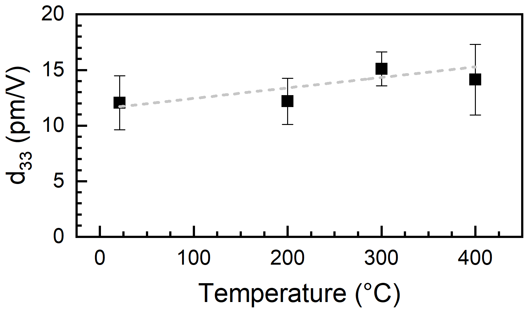
Figure 4 Average values of d₃₃ over temperature. The error bars correspond to the standard deviation of the spatial distribution on the inner part of the sample (see Fig. 3).

5.3 Comparison to literature

As already discussed in Sect. 2.1, Table 1, the literature values at room temperature differ considerably, ranging from 5.7 to 23.1 pm V⁻¹. They thus vary by a factor of more than 4. The data obtained in this study are within this range, at 12.1 pm V⁻¹ at 21 °C and up to 15.1 pm V⁻¹ at elevated temperatures, and are therefore plausible. No clear reason for the wide variation in the literature data could be found. Since the available references often do not provide any information on this, it may also be due to the samples themselves, and each measurement is correct for the given characterization. Possible factors that could influence the piezoelectric constant include the stoichiometry (congruent, near stoichiometric, stoichiometric) and impurities or doping with elements, e.g., Mg or F (Ye et al., 1988). Other factors that might mainly influence the effective piezoelectric constant or the material's polarization are grain boundaries and domains (Gopalan et al., 2007; Meng et al., 2022).

It is striking that the indirectly determined values are consistently lower than the literature values obtained from direct methods involving mechanical contact with the sample. The respective mean values are 7.9 ± 1.6 pm V⁻¹ for the indirect and 16.7 ± 6.3 pm V⁻¹ for the direct methods.

The data obtained from the direct-measurement methods, however, were acquired in contact with the sample. Here, the influence of the measuring equipment can be overestimated, especially for small measured values, and leads to values that are too high (Berg et al., 2003; Vlachová et al., 2015).

In contrast to all other literature values, the values obtained in this study were determined both directly and without contact. Thus, general measurement deficiencies, as described above, should play a minor role here. This is also supported by the fact that our values fall between the indirect- and direct-contact literature data.

A literature comparison of the quality factor determined experimentally in this work is not applicable, as previous investigations of the Q factor of various vibrations of lithium tantalate and lithium niobate have focused on thin layers (Jacob et al., 2003; Jacob et al., 2004; Kadota et al., 2011, 2021; Lu et al., 2021) and thus describe vibrations in the gigahertz range. As far as is known, there are no studies of Q for lithium tantalate in the kilohertz or megahertz range, nor are there any characterizations of Q using interferometry or laser-Doppler vibrometry.

5.4 Outlook

In this study, lithium tantalate (LiTaO₃, LT) is used as a model material for demonstrating the measurement technique. At elevated temperatures, however, LT is generally no longer suitable for use as a sensor or actuator (Turner et al., 1994) due to its low Curie temperature of 600–630 °C (Levinstein et al., 1966; Glass, 1968; Johnston and Kaminow, 1968; Samuelsen and Grande, 1976). Lithium niobate (LiNbO₃, LN), in contrast, has a significantly higher Curie temperature of around 1140 °C (Smolenskii et al., 1966); however, it suffers from stability problems at higher temperatures above 700 °C (Weidenfelder et al., 2012), particularly due to chemical decomposition (Damjanovic, 1998), which could be stabilized by adding LT. In the form of a solid solution, lithium niobate tantalate (LNT) single crystals have the potential to overcome the disadvantages of both individual materials, and LNT is expected to be usable at elevated temperatures above 600 °C (Suhak et al., 2021; Yakhnevych et al. 2024).

5.4.1 Open questions

The objective of this research project was to establish a proof of concept. Naturally, even with a successful initial proof of concept, questions remain unanswered at such an early stage, and there are still untested approaches for further optimizing the new measurement setup. Although the spatially resolved measurement data across the electrode surface show a generally homogeneous distribution, the individual measurement points exhibit greater variability than one might expect based on theory alone. The causes of this are not yet fully understood. One possible explanation is speckles on the electrode surface that distort the LDV measurement signal. This may be caused by electrode degradation or agglomeration, as supported by the fact that this effect appeared to increase over the course of the measurement campaign. However, the influence of the sample holder or the transmission of possible vibrations within the measurement system cannot be entirely ruled out either. Both factors will be investigated more closely through further comparative measurements in future research.

Even if the coupling of additional modes and the influence of mechanical damping can be largely ruled out (see Appendices E, F, G), full-field displacement mapping and modeling would provide detailed insight and further substantiate the discussion. Therefore, we intend to (i) perform spatially resolved LDV scans of the surface displacement at resonance and (ii) combine and compare these with finite-element simulations of the mode shape. A key focus within follow-up works will also be to vary the electrode diameter in order to better understand the influence of boundary effects and clamping effects caused by the unexcited sample edge.

6 Conclusions

This study demonstrates that laser-Doppler vibrometry (LDV) enables direct, non-contact determination of the piezoelectric coefficient d₃₃ in LiTaO₃ with freely vibrating samples of up to 400 °C. Key outcomes are the following:

• i.

  d₃₃ values around 12.1 pm V⁻¹ at 21 °C and up to 15.1 pm V⁻¹ during heating up to 400 °C are determined. These are consistent with the room-temperature literature range when considering method-dependent differences. Temperature-induced changes in d₃₃ within the studied range are small and within the experimental uncertainty; however, a trend toward a slight increase with temperature seems possible.

• ii.

  Measurements were conducted in off-resonant and near-resonant states, using a specially designed low-disturbance sample holder setup that permits nearly free sample vibration and minimizes clamping-induced errors.

• iii.

  A direct, non-contact approach avoids common artifacts associated with indirect methods or contact-mode measurements, such as loading effects, edge constraints, and model-dependent parameter extraction.

• iv.

  The LDV technique shows good agreement with impedance-based characterization for describing the course of admittance or impedance curves in the vicinity of resonances.

• v.

  The successful demonstration of this proof of concept sets the stage for extending LDV-based characterization to other materials, enabling systematic, high-temperature piezoelectric data that are essential for robust design of, e.g., LiTaO₃-based high-temperature devices.

Overall, the LDV-based approach offers a reliable, versatile tool for obtaining direct, high-temperature piezoelectric constants, reducing methodological influences inherent to indirect or contact-based techniques.

Appendix A: Sample characterization

The sample disks were cut out of a Z-oriented lithium tantalate (LiTaO₃) single-crystal wafer from Precision Micro Optics (USA) with a thickness of 523.2 ± 0.5 µm. The thickness is measured using a digital dial gauge, model MarCator 1086R-HR, from Mahr (Germany). The sample was milled into a circular-shaped disk with a diameter of 10 mm using an ultrasonic mill (dama UST 300, Switzerland).

The sample disks are centrosymmetrically coated with keyhole-shaped electrical contacts on both sides using pulsed-laser deposition (PLD) with highly reflective PtRh electrodes with a diameter of approximately 7 mm. The selected deposition parameters (pulse length: 20 ns, pulse energy: 350 mJ, repetition frequency: 30 Hz, deposition time: 40 min) result in layer thicknesses of about 0.8 µm. The layer thickness was determined using a tactile stylus profilometer, Alpha-Step D-600 (USA). Figure 1 shows a scheme of the coated sample from the top (a) and side (b).

Appendix B: Sample setup

When designing the sample holder, particular attention should be paid to two aspects. (i) The piezoelectrically excited sample volume, i.e., the area between the electrodes, must not be clamped at all so that it is not affected by the holder design. The support points must be minimal and located at the outermost point of the samples. This allows for the least possible disturbance to the oscillatory motion in both directions, back and forth. (ii) The sample holder must be movable and rotatable through 180° so that both the front and the back sides can be characterized using LDV without having to remove the sample in between, as each new installation could cause small deviations. Since it must also be stable at high temperatures and electrically insulating, a two-piece design made of aluminum oxide was chosen. The clamping unit, see Fig. 1c, consists of two screw-together ceramic plates with a round cut-out in the middle that is slightly larger than the sample disks. To gently fix the samples, there are four symmetrically arranged protruding clamping points that extend just under 1 mm onto the sample, thus securing it only at these small areas (each approx. 0.4 mm² in size); see Fig. 1c. The rest of the sample surface is not constrained and can move or vibrate completely freely. Pt contact wires are attached to two of these holding points, where the bridges of the keyhole electrodes end, via thin Pt flags (thickness: 100 µm). In this way, the most accurate results possible are achieved, minimizing or compensating for influences and damping caused by the unavoidable sample contact. Since even slight material irregularities and manufacturing tolerances can minimally alter the contact pressure on the sides of the sample, this clamping unit is inserted into a larger, outer suspension, which allows the sample to be measured from both sides without removing it from the primary clamping unit. This enables direct measurement and averaging across both directions of vibration, eliminating the need for compensation as required for samples positioned on a stiff surface, resulting in asymmetrical oscillations only in one direction.

Appendix C: Conducting and evaluating the LDV measurements

The general setup of the laser-Doppler vibrometer (LDV) used for this research is described in detail by Schmidtchen et al. (2018), Wulfmeier et al. (2021), and Schewe et al. (2023).

The sample disks are piezoelectrically excited by applying a sinusoidal voltage signal emitted by a function generator, Hameg HMF2525 (Germany). The peak-to-peak voltage was varied between 1 and 10 V; however, the later discussion focuses on the 10 V measurements as those exhibit the highest SNR.

A continuous laser beam (λ=633 nm) is emitted by the LDV, directed towards the electrode surface, reflected, and then directed into the detector where it is superimposed with the reference beam. Hereby, adjustable tilt mirrors allow for the precise adjustment of the laser path so that the whole sample surface can be scanned. The detector signal, i.e., the phase shift of the laser beams (measurement and reference beam), is forwarded to the decoder (displacement or velocity decoder), which in turn forwards the measurement results to an oscilloscope (PCI-5122, National Instruments, USA), which also measures the excitation voltage. The displacement decoder (OFV-5000, Polytec, Germany, resolution: R_D=50 nm V⁻¹) can be used up to excitation in the kilohertz range; for measurements at megahertz excitation, a velocity decoder (OFV-9000, Polytec, Germany, resolution: R_V=100 mm (sV)⁻¹) has to be used instead. The LDV decoder translates this interference pattern into a time-resolved voltage signal that is converted into a frequency-resolved voltage signal using a fast Fourier transformation (FFT). The maximum displacement can then be determined from this according to the data evaluation approach described in Kohlmann et al. (2024).

There are generally two measurement modes available: (i) variation of the excitation frequency at a constant local measurement point and (ii) lateral scan across the sample surface at a constant excitation frequency. In the latter case, a further distinction is made between whether the measurement takes place near the resonance frequency or in an off-resonant state.

The parameters used in this study for (i) were a measuring range of approximately 10 kHz with a point density of approximately 90 Hz. For verification purposes, parallel comparative measurements were performed on the same sample and in an identical test setup using a vector network analyzer (HP E5100A, USA), which had previously been calibrated using an open-short-load (OSL) approach (Wulfmeier et al., 2013).

For (ii), the LDV measurements were performed using a grid consisting of a horizontal and vertical measuring line, each with 13 points at equidistant intervals above the electrode. The lateral point spacing is thus slightly less than 0.6 mm. The grid can be seen in Fig. 1c. Before and after each LDV measurement, a waiting time of at least 100 ms is set after the start or end of the excitation. Exciting the sample shortly before the measurement serves to prevent any disturbances during the settling of the sample. Not exciting the sample between measurements serves, on the one hand, to avoid permanently stressing the sample and, on the other hand, to allow it to relax in the meantime in order to rule out interference with the previous measurement frequency. For statistical reasons, five individual measurements were averaged per measurement point.

Measurements were performed in an off-resonant state at 55 kHz and near the resonance frequency of the thickness vibration of the sample at 5.8 MHz. The piezoelectric coefficient was measured at room temperature, 200, 300, and 400 °C, each under ambient atmospheric conditions in a tube furnace (HTSS 75-180/16, Gero GmbH, Germany).

Appendix D: Calculation of sample displacement from the LDV measurement signal

As mentioned in the previous section, a laser-Doppler vibrometer outputs an interference pattern. The LDV decoder translates this into a time-resolved voltage signal, which is converted into a frequency-resolved voltage signal using a fast Fourier transform (FFT). The FFT is an algorithm that can be used to decompose a discrete signal, in this case the voltage signal over time, into discrete components, in this case the contributions of the individual frequencies to the voltage signal (Kohlmann et al., 2023, 2024). The measured displacement can then be determined from this. Depending on whether a displacement decoder with resolution R_D or a velocity decoder with resolution R_V is used, the maximum of the voltage signal U_LDV,max is proportional to the measured displacement on the examined surface d in the measurement direction at this frequency or the speed v of the displacement:

$$\begin{array}{}\text{(D1)}& {\displaystyle }s=U_{\mathrm{LDV},\max }{R}_{\mathrm{D}}\text{(D2)}& {\displaystyle }v=U_{\mathrm{LDV},\max }{R}_{\mathrm{V}}.\end{array}$$

Since an oscillating object reaches its amplitude once per oscillation, the speed of the oscillation is the product of s and the angular velocity ω, i.e., the total number of oscillations per second:

$$\begin{array}{}\text{(D3)}& v=s\mathit{\omega }=s\mathrm{2}\mathit{\pi }f,\end{array}$$

resulting in the displacement

$$\begin{array}{}\text{(D4)}& s={\displaystyle \frac{v}{\mathrm{2}\mathit{\pi }f}}={\displaystyle \frac{U_{\mathrm{LDV},\max }}{\mathrm{2}\mathit{\pi }f}}{R}_{\mathrm{V}}.\end{array}$$

As stated before, the vibration is bidirectional. Therefore, the total displacement S is the sum of the displacement signals on the front and back side of the sample:

$$\begin{array}{}\text{(D5)}& S=s_{\mathrm{front}}+s_{\mathrm{back}}.\end{array}$$

If the piezoelectric vibration is in the direction of the laser beam, then the maximum displacement is equal to the measured displacement and, thus, directly proportional to the LDV voltage signal. As this work focuses on the d₃₃ component of a Z-cut LiTaO₃ crystal, this condition is fulfilled here.

Appendix E: Influence of additional vibration modes on LDV measurements

Laser-Doppler vibrometry (LDV) selectively captures signal components at the excitation frequency (55 kHz and 5.8 MHz in this work) and its higher harmonics, filtering out frequencies outside this narrow band (≈ 0.01 % of the excitation frequency). Interfering waves would thus need to couple precisely at the excitation frequency to affect the measurement signal.

The most relevant potential interfering modes are flexural modes of thin plates. For the given geometry and reasonable material parameters (E≈160 GPa, ρ≈7450 kg m⁻³, ν≈0.33), the second and third flexural modes occur at approximately 25 and 59 kHz, respectively, calculated according to Colwell and Hardy (1937), Leissa (1969), Kollmann et al. (2005), and Steinke (2015). In between, there is the (0,1) mode at approximately 43 kHz. The applied excitation frequency of 55 kHz therefore does not coincide with any flexural resonance. At the resonance frequency of 5.8 MHz, the modes are of a very high order with numerous nodal lines, resulting in negligible absolute displacement.

Thickness shear vibrations, which do not cause any thickness deflection, should nevertheless be mentioned for the sake of completeness. For the given samples they occur at approximately 3.9 MHz – nearly 2 orders of magnitude above the static measurements (55 kHz) and more than 30 % below the resonance measurements (5.8 MHz). Their higher harmonics lie significantly above this frequency and thus far from the measurement range. Lateral modes, starting from 6.0 MHz, are also well outside the evaluated frequency band.

Experimentally, the data show no resonance-like features such as amplitude enhancement or phase shifts in the investigated frequency range. Furthermore, the electromechanical coupling of the applied field to flexural modes is intrinsically weak, as uniform strain is induced via the d₃₃ coefficient, whereas flexural motion requires a strain gradient across the thickness. This further justifies neglecting flexural modes in the present analysis and is consistent with established descriptions of plate mechanics and piezoelectric coupling (Timoshenko and Woinowsky-Krieger, 1959; IEEE, 1988).

In addition, spurious components could also be present in the measurement signal. We cannot calculate or rule these out with complete certainty. To address this, preliminary characterization was performed using a network analyzer, and only those resonators that did not exhibit any significant spurious modes in their resonance frequency spectrum were used.

Appendix F: Influence of boundary conditions, piezoelectric coupling, and deformation modes

F1 Boundary constraints and clamping effects

The resonator sample is mounted at four small nose tabs along the outermost edge, ensuring near-free boundary conditions and minimal lateral restraint. Taking material parameters from Warner et al. (1967), the local clamping stress (6–12 kN m⁻²) is well below the piezoelectric stall stress (64 kN m⁻²) and acts only at the non-electrode edge, leaving the centrally excited region virtually unaffected.

F2 In-plane piezoelectric coupling ($d_{\mathrm{31}}/d_{\mathrm{15}}$ contributions)

For a laterally unconstrained piezoelectric plate, the thickness strain

$$\begin{array}{}\text{(F1)}& S_{\mathrm{3}}=d_{\mathrm{33}}{E}_{\mathrm{3}}+S_{\mathrm{13}}{T}_{\mathrm{1}}+S_{\mathrm{13}}{T}_{\mathrm{2}}\end{array}$$

is governed almost exclusively by the d₃₃ coefficient, as lateral stresses T₁ and T₂ are zero. Poisson-induced in-plane strains do not significantly contribute to out-of-plane motion, since the material can expand laterally without restriction (Ikeda, 1990; Flax et al., 1981). Thus, the out-of-plane displacement amplitude is only weakly affected by the Poisson ratio.

F3 Warpage and bending contributions

The measured 5.8 MHz resonance is sharply peaked and spatially uniform, with no evidence of large-scale curvature or asymmetric mode components in the LDV maps. This confirms that the response is dominated by thickness-extensional vibration, with negligible bending contributions, which is consistent with Rosen et al. (2005) (see also Appendix E).

Appendix G: Contribution of electrode-free regions

In piezoelectric resonators, the electromechanical conversion is almost entirely confined to the regions coated with electrodes, since the measured current corresponds to a spatially weighted integral over these areas (Lowe, 1995). In the off-resonant regime, the mechanical displacement that originated from the applied electric field varies smoothly, and contributions from electrode-free regions can be widely neglected as they enter only indirectly via elastic coupling and decay strongly with distance, consistent with the properties of elastic Green's functions and wave solutions in continuous media. For example, in thickness shear mode resonators, the amplitude at the edge drops to ∼ 0.08 of the maximum (Martin and Hager, 1989). This behavior arises from the modal expansion of harmonically driven linear elastic systems, where no single mode dominates, and the spatial response remains smooth. This behavior follows directly from the modal expansion of linear elastic systems driven harmonically (Ern and Guermond, 2004).