Data-driven vibration-based bearing fault diagnosis using non-steady-state training data

This paper presents the extension of an empirical study in which a universally applicable fault diagnosis method is used to analyse vibration data of bearings measured with accelerometers. The motivation for extending the previously published results was to provide a profound analysis of the proposed approach with regard to a more feasible training scenario for real applications. For a detailed assessment of the method, data were acquired on two different test beds: a gearbox test bed equipped with various bearings at different health states and an accelerated lifetime (ALT) test bed to degrade a bearing and introduce an operational fault. Features were extracted from the raw data of two different accelerometers and used to monitor the actual health state of the bearings. For that purpose, feature selection and classifier training are performed in a supervised-learning approach. The accuracy is estimated using an independent test dataset. The results of the gearbox test bed data show that the training of the method can be performed with non-steady-state data and that the same feature set can be used for different revolution speeds if a small decrease in accuracy is acceptable. The results of the ALT test bed show that the same features that were identified in the gearbox test start to change significantly when the bearing starts to degrade. Thus, it is possible to observe the identified features for applying predictive maintenance.

1 Introduction

Manufacturing companies continuously try to increase their productivity, by avoiding machine downtime among other things. The former involves considerable costs because of the resulting loss of turnover. Monitoring the condition of, for instance, bearings and gears plays a vital role in the maintenance programme of rotating machines. Early fault detection could allow for moving from a time-based preventive-maintenance programme to a condition-based predictive-maintenance strategy and reducing unexpected machine downtime and cost.

Vibration-based condition monitoring is an established approach that has been employed by industries for many years in their maintenance programmes (Randall, 2011). However, up to this day, machine operators often still base their maintenance decisions on data from the periodical and manual inspection of single machines, which does not always result in correct conclusions. The common practice is that vibration measurements are periodically recorded using portable vibration sensors, and measurement signals are analysed by an expert to interpret the machine's health condition. This approach can, however, lead to serious misinterpretation, where rapidly growing impairments could be missed.

A continuous condition-monitoring approach enables early detection of machine faults. In this way, the machine condition is continuously tracked, and total failures can be anticipated in advance, hence allowing appropriate maintenance actions. Despite their advantages, continuous monitoring programmes are still not well adopted by industry. Firstly, this is because it often involves a high investment cost. Although recent advancements in sensor, acquisition and processing hardware have demonstrated cost-effective solutions (Albarbar et al., 2008; Ompusunggu et al., 2018), the economic benefit of the investment is still not clear and hard to quantify. Secondly, this is because many of those systems still require an expert to interpret the analysis results. Finally, this is also because it is not straightforward to select the most appropriate condition-monitoring method for a specific application.

A wide range of vibration-based bearing fault detection methods have been proposed in the literature (Henriquez et al., 2014; Sait and Sharaf-Eldeen, 2011; Wang et al., 2017; Zarei et al., 2014). Approaches that utilize time domain features (e.g. crest factor and kurtosis; Barbini et al., 2017), frequency and cepstral-domain features (e.g. envelope analysis and cepstral coefficients; Borghesani et al., 2013) usually assume stationary machine conditions. Other methods such as cyclostationary analysis (i.e. second-order technique in the frequency domain; Dalpiaz et al., 2013; Hu et al., 2019) and time–frequency domain analysis (e.g. Wigner–Ville distribution, Hilbert–Huang transform and wavelet-transform-based features; Bajric et al., 2016) are more appropriate for non-stationary processes. Some of those methods are purely data driven, whereas others use the physical relation between the bearing geometry, the rotational shaft speed and the bearing-specific fault frequencies associated to the impulse behaviour introduced by bearing faults.

In this paper, we present a purely data-driven method that extracts a large number of features from vibration data of accelerometer measurements and selects and classifies these features in a supervised-learning approach. Training and test data were acquired at two different bearing test beds: a gearbox setup that can be equipped with bearings of different degradation statuses and a simple rotating shaft with a bearing under certain radial loads for accelerated degradation. However, the method does not address one specific application with certain requirements of the application. We applied the same basic idea to very different applications like fault diagnosis in a hydraulic accumulator loading circuit or oscillation detection. In both cases, we obtained satisfying accuracy values. In any case, the limitation of the method is that it requires information-rich training data of the underlying system to select meaningful features and train suitable classifiers. In this context, information-rich means that the training data have to contain the different possible (fault) states of the application as well as different operation modes. There are of course general requirements that hold for fault detection in most applications, such as the desire to obtain a high detection accuracy and the ability to detect faults under all relevant operational conditions. Both of them are tackled implicitly for the specific application of this paper by the main goals that are stated below.

The basics of the proposed method were already compared to two state-of-the-art methods for bearing monitoring in Ooijevaar et al. (2019). It proved that it can compete with the other methods, although those incorporate specific knowledge about the monitored bearing, while the proposed method is purely data driven. Of course, there are also some drawbacks of the proposed method compared to the other state-of-the-art methods, for instance the requirement of sufficient training data for different states and operation modes.

In contrast to Ooijevaar et al. (2019), the goal of this paper is to analyse if a more feasible training scenario is possible. Therefore, it is investigated if it is sufficient to acquire training data with linearly increasing speed instead of many different steady-state speed levels to save time for training data acquisition. It is also investigated if the same feature set can be used for different revolution speeds of the bearing to make it applicable to different speeds without adapting the feature set.

The paper is structured as follows: in Sect. 2, the problem is briefly stated, and the experimental setup is introduced. The classification method is described in detail in Sect. 3, and Sect. 4 provides test results. Finally, Sect. 5 gives the conclusions of the work.

2 Problem statement and experimental setup

In this paper, a previously proposed method (Ooijevaar et al., 2019) for bearing fault detection based on vibration measurements is further analysed with regard to a more feasible training scenario for real-world applications. For that purpose, it is firstly investigated if training data can be acquired using measurements with linearly increasing speed instead of acquiring data at many different steady-state speed levels. That saves a significant amount of time for training data acquisition. Secondly, it is investigated if the same feature set can be used for different revolution speeds of the bearing. That makes the approach more universally applicable, since there is no need to adapt the feature set to the revolution speed.

Since the paper deals with applying the proposed method to bearing fault detection, it is of essential importance to know the underlying physical system. Hence, this section provides a detailed explanation of the experiments and the measured data. Two types of experiments have been performed: (i) an accelerated lifetime test (ALT) of a ball bearing on a single-shaft drive train setup and (ii) a test on a more complex gearbox setup including bearings with various faults. In both test setups, the vibrations of the bearing are measured by accelerometers. These vibration data are used to detect the faults in a machine-learning approach. The tests are described in the next two subsections.

2.1 Accelerated lifetime test

The accelerated lifetime test allows for creating an operational fault in a bearing. This test differs from other studies on the fact that those are often limited to artificially induced faults. Moreover, the fault evolution and accumulation can be monitored during the accelerated lifetime. The experimental setup used to perform the accelerated lifetime test is shown in Fig. 1. The setup comprises of a single shaft with a test bearing. The shaft is supported with the help of a support bearing on each side. A hydraulic cylinder is used to apply a radial load to the test bearing up to a maximum of 10 kN. The test bearing is oil lubricated by an internal oil bath. Two air fans are installed to cool the setup and avoid overheating of the bearing. The setup is driven by a motor at a fixed rotation speed of 1500 rpm.

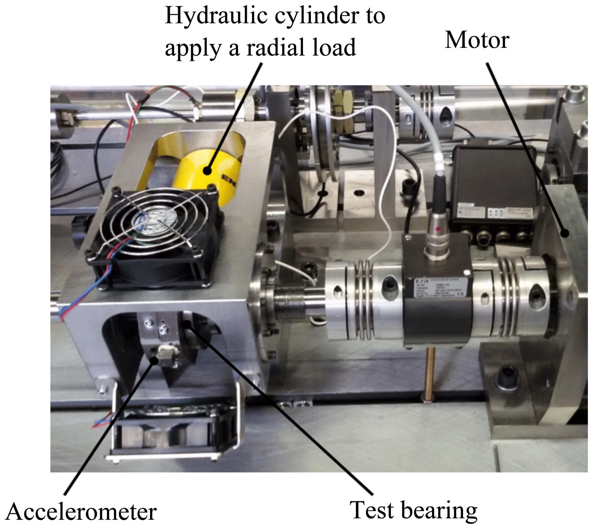
Figure 1 The drive train setup used to reduce the lifetime of a bearing to less than 1 d, allowing for the generation of vibration data during the accumulation of an operational bearing fault.

The test procedure is schematically illustrated in Fig. 2. Vibration measurements were performed under a nominal radial load of 1.5 kN (i.e. 10 % of the dynamic load rating). The radial load was temporarily increased to 9.0 kN (i.e. 65 % of the dynamic load rating) to accelerate the degradation of the bearing. In the beginning, the interval of increased load was 20 min, but this had been reduced as soon as the first indication of an incipient fault was noticed in the measured vibration responses. In total, 30 vibration measurements were performed at the nominal 1.5 kN load condition, and 29 vibration measurements were performed at the high 9.0 kN radial load. The accelerated lifetime test was stopped when a vibration peak level of ±50 g was reached.

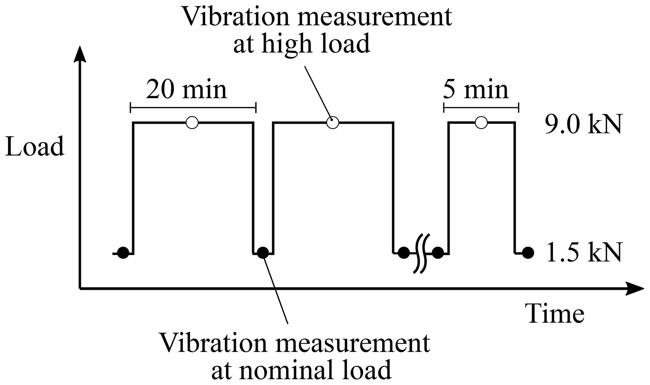
Figure 2 The load was temporarily increased from 1.5 to 9 kN to accelerate the lifetime of the bearing.

The applied radial load, the radial vibrations in the loading direction and the temperature of the bearing housing were measured during the test. The machine vibrations were measured using a piezo-film ACH-01-03 accelerometer and sampled at 12.8 kHz by an embedded acquisition platform. In each measurement, 20 s of data were acquired. The acquisition platform consists of a BeagleBone Black single-board computer with a Linux operating system, supplemented with a customized six-channel interface. This embedded platform is used as a compact, open, scalable and cost-effective data acquisition system.

The accelerated lifetime test was performed on a FAG 6205 ball bearing. Before the start of the test, a small indentation (see Fig. 3) with a diameter of 230 µm was created in the inner race using a Rockwell C hardness tester. This indentation is used as a local stress riser and represents a local plastic deformation caused by, for instance, a contamination particle. Subsequently, the accelerated lifetime test was performed for several hours. Although bearings can fail in many different ways, the indentation triggers the bearing to fail in a more repeatable way. The test was stopped when severe rolling contact surface fatigue occurred at the inner race (Halme and Andersson, 2009). The start and the end condition of the inner race of the test bearing are shown in Fig. 3.

Figure 3 The indentation at the bearing inner race was used as the start condition, and the surface fatigue fault at the inner race was introduced by the accelerated lifetime test.

Only a single dataset has been used in this paper. However, the accelerated lifetime test has been performed several times as part of other research by the authors. They have all resulted in similar surface fatigue faults at the inner race of the test bearing.

2.2 Gearbox test

The second test performed in this study was an industrially representative gearbox setup. Figure 4 shows a photograph and a schematic top view of the gearbox setup. The test setup consists of (i) an induction electric motor, (ii) a gearbox and (iii) a magnetic brake. The motor is controlled by a variable-frequency drive (VFD) with either a stationary mode or a transient mode (run-up or run-down mode). The motor speed can be controlled from 0 to 3000 rpm. The gearbox input shaft is connected to the motor through a flexible coupling, while the gearbox output shaft is directly coupled to the brake. The torque applied to the brake can be adjusted by the controller from 0 to 50 Nm.

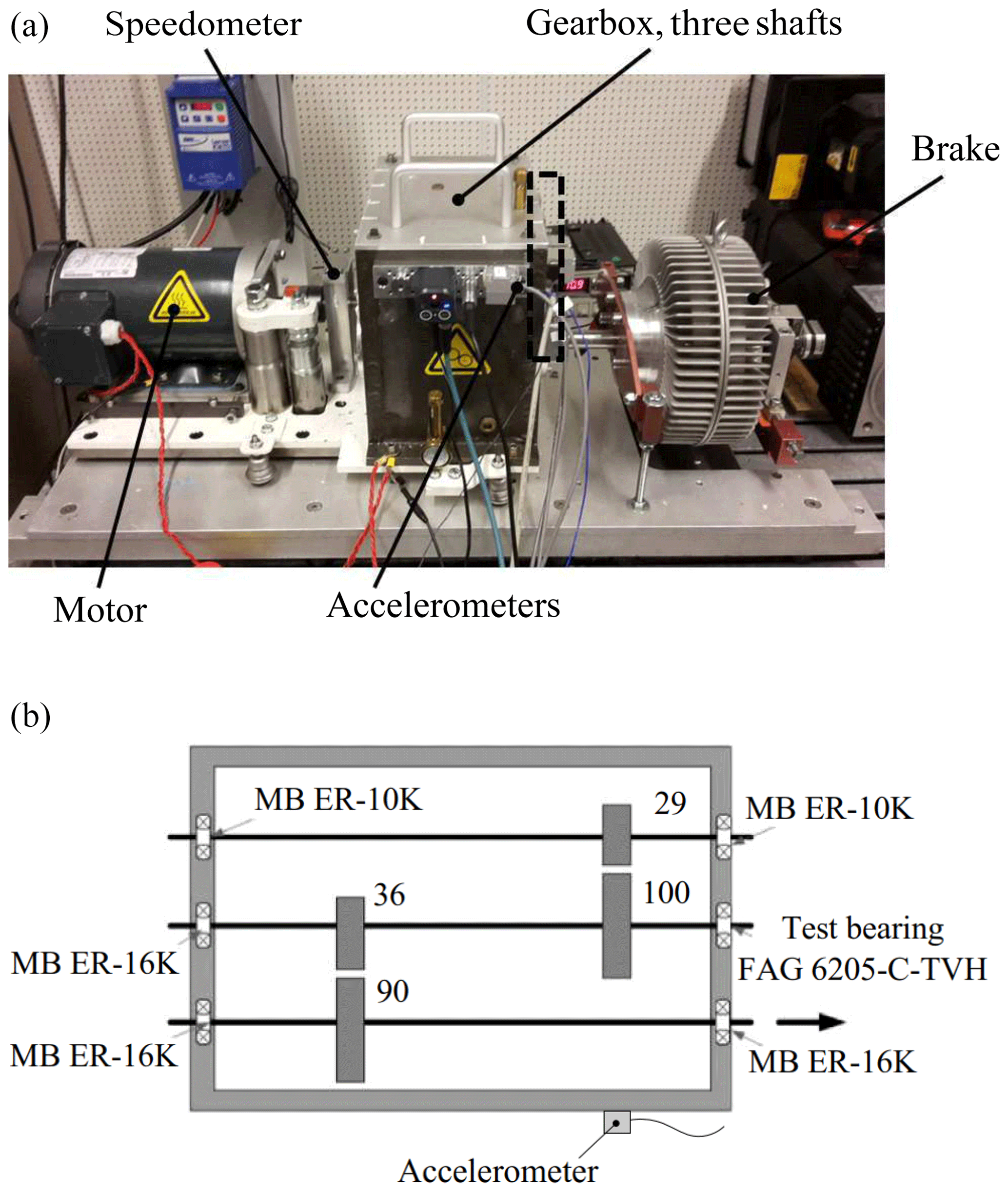
Figure 4 Gearbox setup comprising a motor, three-shaft gearbox and brake to introduce a load.

As illustrated in Fig. 4, the gearbox comprises of three parallel shafts connected through contacting spur gear pairs. Note that the number of gear teeth is indicated in the figure. Hence the total reduction factor from the input to the output shaft is equal to $(\mathrm{100}/\mathrm{29})\times (\mathrm{90}/\mathrm{36})=\mathrm{8.62}$. The input shaft is supported by MB ER-10K deep-groove ball bearings, while the other shafts are supported by MB ER-16K deep-groove ball bearings. For simulating a healthy or faulty state on the gearbox, the right-side bearing housing that supports the second shaft is equipped either with a healthy or a damaged FAG 6205-C-TVH ball bearing.

Two healthy bearings and three faulty bearings with different inner race faults were tested. An indentation fault with a diameter of 490 µm was created using an Rockwell C hardness tester. Two other bearings with operational faults were created using the accelerated lifetime test setup as described in Sect. 2.1. The healthy bearings are referred as “Healthy1” and “Healthy2”, while the faulty bearings are referred as “Indent”, “Faulty1” and “Faulty2”, in order of increasing severity; these are illustrated in Fig. 5.

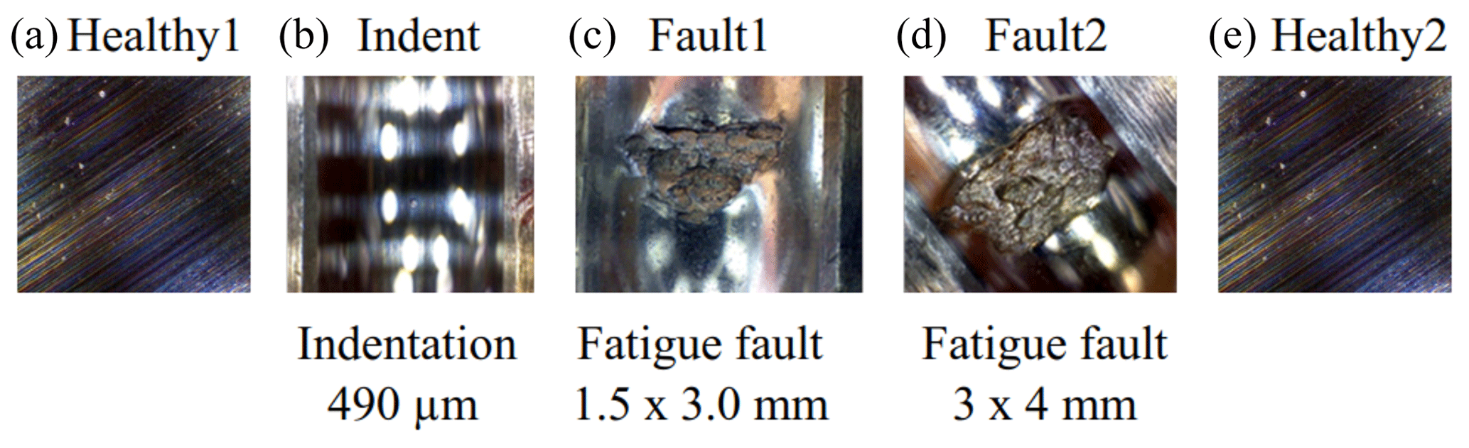
Figure 5 Five bearing states tested on the gearbox setup comprising two healthy bearings and three faulty bearings with different severities.

For each healthy or faulty state, two operating conditions were imposed on the gearbox setup, namely two different motor speeds of 1500 and 3000 rpm. The brake torque was kept constant at 50 Nm. Because of the transmission ratio, the rotational speed of the second shaft is 29∕100 lower than that of the motor speed, while the torque applied on the second shaft is 36∕90 lower than that of the brake torque. Hence, for the imposed operating conditions, the rotational speeds of the second shaft were 435 and 870 rpm, while the torque applied to the second shaft was 20 Nm. A high-end PCB (picocoulomb; manufacturer PCB Piezotronics) accelerometer and a low-cost MEMS (microelectromechanical-system) accelerometer were mounted on the gearbox housing as shown in Fig. 4. The vibration signals were sampled at 50 kHz using a Dewesoft data acquisition system. For each operating condition, 10 operations of 20 s each were repeated. Furthermore, for each of the five tested bearing states, three ramp-up measurements were conducted. In these ramp-up measurements, the motor speed was increased linearly from 0 to 3000 rpm within 40 s. The ramp-up measurements are used to investigate the first and main aim of this paper, i.e. reducing measurement effort for training data acquisition. It is obvious that conducting 40 s of ramp-up measurements saves a significant amount of time compared to conducting steady-state measurements for several seconds at many revolution levels. All data are then processed using scripts written in MATLAB.

3 Classification method

The fault diagnosis approach presented here is a purely data-driven one; i.e. it incorporates no physical knowledge about the monitored system. This makes it on one hand much more flexible and applicable to many other kinds of systems, machines or components. On the other hand, incorporating extra knowledge usually improves the diagnostic ability of a condition-monitoring system and reduces the necessary amount of training data.

The proposed method applies a supervised-learning approach to annotated measurement data. In the presented application, accelerometers measure vibrations that are caused by the bearing to be monitored. For this purpose, the accelerometer is mounted at the housing of the bearing (see for instance Fig. 1). Since the fault state in the gearbox setup is known, annotated data for classifier training are available.

The training procedure of the proposed method consists of three steps:

• feature extraction from annotated data

• feature selection

• classifier training.

The evaluation procedure for new data consists of two steps:

• extraction of the features selected in the training procedure

• classifier evaluation.

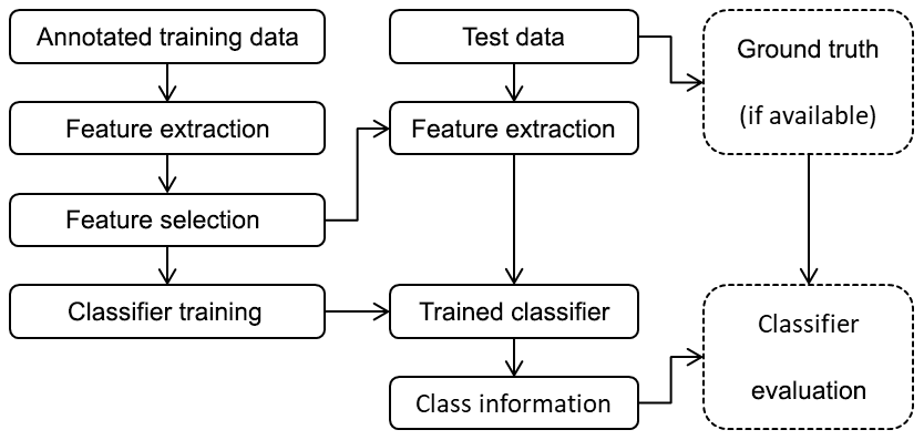
All steps are described in more detail in the following subsections. Moreover, the combination of training and test procedures is summed up in Fig. 6. From the annotated training data, features are extracted, and the most significant features for the classification task are selected. With these features, a classifier is trained. From the test data, the features that were selected before are extracted. The trained classifier is applied to the features to obtain the estimated class information for the test data. If the ground truth of the test data is available, it can be used together with the estimated class information to evaluate the classifier (confusion matrix, accuracy, etc.; de Ridder et al., 2017).

Figure 6 Block diagram of the proposed method.

3.1 Feature extraction

In the first step, a large number of features is extracted in a sliding-window approach from the raw accelerometer signals. Feature extraction for vibration analysis has been discussed in numerous publications; extensive reviews can be found for instance in Wang et al. (2017) and Singh and Vishwakarma (2015). The extraction of typical statistical features in the time domain is described in Sharma and Parey (2016), Lei et al. (2007), Shen et al. (2013), Decker and Lewicki (2003), Alattas and Basaleem (2007), Boldt et al. (2013), Jalil et al. (2013), Suma and Gurumurthy (2010), and Kollialil et al. (2013). Features in the time–frequency and frequency domains are proposed and investigated in Sharma and Parey (2016), Lei et al. (2007), Alattas and Basaleem (2007), and Boldt et al. (2013). Typical symptom parameters in the frequency domain for rotating machinery are extracted in Wang and Chen (2007). Adopting the spectral kurtosis for vibration monitoring is examined in Rao (2015) and Antoni and Randall (2006). In McClintic et al. (2000) and Assaad et al. (2014), features of residual and difference signals are extracted by using for instance autoregressive models. Features in the wavelet domain are introduced in Heidari Bafroui and Ohadi (2014), Jafarizadeh et al. (2008), Bajric et al. (2016), and Kollialil et al. (2013). Satyam et al. (1994) and Konstantin-Hansen and Herlufsen (2010) examine vibration analysis in the cepstral domain. The application of synchronous time averaging is demonstrated for instance in McFadden and Toozhy (2000). We implemented a broad selection of the proposed features to analyse the measured data. Overall, 83 features were extracted. Amongst the finally selected features of a time series $x=x_{\mathrm{1}},x_{\mathrm{2}},\mathrm{\dots },x_n$ were for instance the root mean square (RMS; Sharma and Parey, 2016) as

$$\begin{array}{}\text{(1)}& x_{\mathrm{rms}}=\sqrt{{\displaystyle \frac{\mathrm{1}}{n}}\cdot \sum _{i=\mathrm{0}}^n{x}_i^{\mathrm{2}}}\end{array}$$

or the interquartile range (Kollialil et al., 2013) as

$$\begin{array}{}\text{(2)}& x_{\mathrm{iqa}}={\widehat{x}}_{\mathrm{0.75}}-{\widehat{x}}_{\mathrm{0.25}},\end{array}$$

where

$$\begin{array}{}\text{(3)}& {\widehat{x}}_p=\left\{\begin{array}{ll}\frac{\mathrm{1}}{\mathrm{2}}\left(y_{n\cdot p}+y_{\left(n\cdot p\right)+\mathrm{1}}\right)& \text{if }n\cdot p\in \mathbb{N}\\ y_{⌊n\cdot p+\mathrm{1}⌋}& \text{if }n\cdot p\notin \mathbb{N}\end{array}\right.\end{array}$$

and $y_{\mathrm{1}}\le y_{\mathrm{2}}\le \mathrm{\dots }\le y_n$ are the sorted values of x.

Also the symptom parameters (Wang and Chen, 2007) of

$$\begin{array}{}\text{(4)}& p_{\mathrm{2}}=\sqrt{{\displaystyle \frac{{\sum }_{i=\mathrm{1}}^N{f}_i^{\mathrm{4}}\cdot S\left(f_i\right)}{{\sum }_{i=\mathrm{1}}^N{f}_i^{\mathrm{2}}\cdot S\left(f_i\right)}}}\end{array}$$

and

$$\begin{array}{}\text{(5)}& p_{\mathrm{4}}={\displaystyle \frac{\mathit{\sigma }}{\stackrel{\mathrm{‾}}{f}}},\end{array}$$

where f_i, $i=\mathrm{1},\mathrm{\dots },N$ are the frequency bins, S(f_i) is the power spectrum,

$$\begin{array}{}\text{(6)}& \mathit{\sigma }=\sqrt{{\displaystyle \frac{{\sum }_{i=\mathrm{1}}^N{\left(f_i-\stackrel{\mathrm{‾}}{f}\right)}^{\mathrm{2}}\cdot S\left(f_i\right)}{N-\mathrm{1}}}}\end{array}$$

and

$$\begin{array}{}\text{(7)}& \stackrel{\mathrm{‾}}{f}={\displaystyle \frac{{\sum }_{i=\mathrm{1}}^N{f}_i\cdot S\left(f_i\right)}{{\sum }_{i=\mathrm{1}}^{N}S\left(f_i\right)}},\end{array}$$

are amongst the top features. However, for confidentiality reasons we are not allowed to name the exact features that were chosen in each particular test. Therefore, we use abstract feature numbers in the following sections.

3.2 Feature selection

In the next step of the supervised-learning approach, the dimensionality of the feature space is reduced to avoid the curse of dimensionality (Bellman, 2003). Therefore, the significant features are identified by feature selection procedures as described in Guyon and Elisseeff (2003). In particular, a standard forward-selection-filter algorithm selecting one feature per step was applied. As the selection criterion in each step of forward selection, we use the robust Dy–Brodley distance measure (Dy and Brodley, 2004). Assuming a dataset with C∈ℕ classes in a k-dimensional feature space, the feature values for each class can be represented as a matrix of ${\mathbf{X}}_c\in {\mathbb{R}}^{n_c\times k}$, $c\in \left\{\mathrm{1},\mathrm{\dots },C\right\}$, with n_c∈ℕ denoting the number of samples for class c. Then μ_c∈ℝ^k and ${\mathbf{\Sigma }}_c\in {\mathbb{R}}^{k\times k}$, $c\in \left\{\mathrm{1},\mathrm{\dots },C\right\}$, denote the mean values and covariance matrices of each class c, and μ∈ℝ^k denotes the mean value over all classes. Defining the within-scatter ${\mathbf{S}}_{\mathrm{W}}\in {\mathbb{R}}^{k\times k}$ as

$$\begin{array}{}\text{(8)}& {\mathbf{S}}_{\mathrm{W}}=\sum _{c=\mathrm{1}}^C{\displaystyle \frac{n_c}{n}}\cdot {\mathbf{\Sigma }}_c\end{array}$$

and the between scatter ${\mathbf{S}}_{\mathrm{B}}\in {\mathbb{R}}^{k\times k}$ as

$$\begin{array}{}\text{(9)}& {\mathbf{S}}_{\mathrm{B}}=\sum _{c=\mathrm{1}}^C{\displaystyle \frac{n_c}{n}}\cdot {\left({\mathit{\mu }}_c-\mathit{\mu }\right)}^{\mathrm{T}}\cdot \left({\mathit{\mu }}_c-\mathit{\mu }\right),\end{array}$$

where

$$\begin{array}{}\text{(10)}& n=\sum _{c=\mathrm{1}}^C{n}_c,\end{array}$$

the Dy–Brodley distance measure is finally defined as

$$\begin{array}{}\text{(11)}& J=\text{tr}\left({\mathbf{S}}_{\mathrm{W}}^{-\mathrm{1}}\cdot {\mathbf{S}}_{\mathrm{B}}\right).\end{array}$$

Feature selection is stopped when the relative gain of the selection criterion falls below 1 %. We also performed tests with the Mahalanobis distance (McLachlan, 1999) as the selection criterion; however, both distance measures resulted in the same feature sets.

3.3 Classifier training

After feature extraction and selection, a classifier is trained in the feature space. For that purpose, we use linear and quadratic discriminant analysis (Hastie et al., 2009; de Ridder et al., 2017).

In this classification approach, the class conditional distributions of a new data sample x∈ℝ^k are modelled as $P\left(\mathit{x}|c=c_i\right)$ for each class $c_i\in \left\{\mathrm{1},\mathrm{\dots },C\right\}$. By using Bayes' rule of

$$\begin{array}{}\text{(12)}& \begin{array}{rl}P\left(c=c_i|\mathit{x}\right)& ={\displaystyle \frac{P\left(\mathit{x}|c=c_i\right)\cdot P\left(c=c_i\right)}{P\left(\mathit{x}\right)}}\\ & ={\displaystyle \frac{P\left(\mathit{x}|c=c_i\right)\cdot P\left(c=c_i\right)}{{\sum }_{c_j=\mathrm{1}}^{C}P\left(\mathit{x}|c=c_j\right)\cdot P\left(c=c_j\right)}}\end{array}\end{array}$$

and selecting the class c_i with highest conditional probability, a class prediction can be made. In the application example of this paper, the classes are “Healthy”, “Indent” and “Fault”. In discriminant analysis, P(x|c) is modelled as a multivariate normal distribution with density

$$\begin{array}{}\text{(13)}& \begin{array}{rl}P& \left(\mathit{x}|c=c_i\right)=\\ & {\displaystyle \frac{\mathrm{1}}{{\left(\mathrm{2}\mathit{\pi }\right)}^{\frac{k}{\mathrm{2}}}\cdot {\left|{\mathbf{\Sigma }}_{c_i}\right|}^{\frac{\mathrm{1}}{\mathrm{2}}}}}\cdot {\mathrm{e}}^{-\frac{\mathrm{1}}{\mathrm{2}}{\left(\mathit{x}-{\mathit{\mu }}_{c_i}\right)}^{\mathrm{T}}\cdot {\mathbf{\Sigma }}_{c_i}^{-\mathrm{1}}\cdot \left(\mathit{x}-{\mathit{\mu }}_{c_i}\right)},\end{array}\end{array}$$

where the prior probabilities P(c=c_i), the class mean values ${\mathit{\mu }}_{c_i}$ and the class covariance matrices ${\mathbf{\Sigma }}_{c_i}$ are estimated from training data. Equation (13) represents the quadratic case of discriminant analysis. In the linear case, the normal distributions for each class are assumed to have the same covariance matrix, i.e. ${\mathbf{\Sigma }}_{c_i}=\mathbf{\Sigma }$ for $c_i\in \left\{\mathrm{1},\mathrm{\dots },C\right\}$.

The validity of using normally distributed classifiers was checked by normal probability plots of the feature vectors (see for instance the feature interquartile range for two states in Fig. 7).

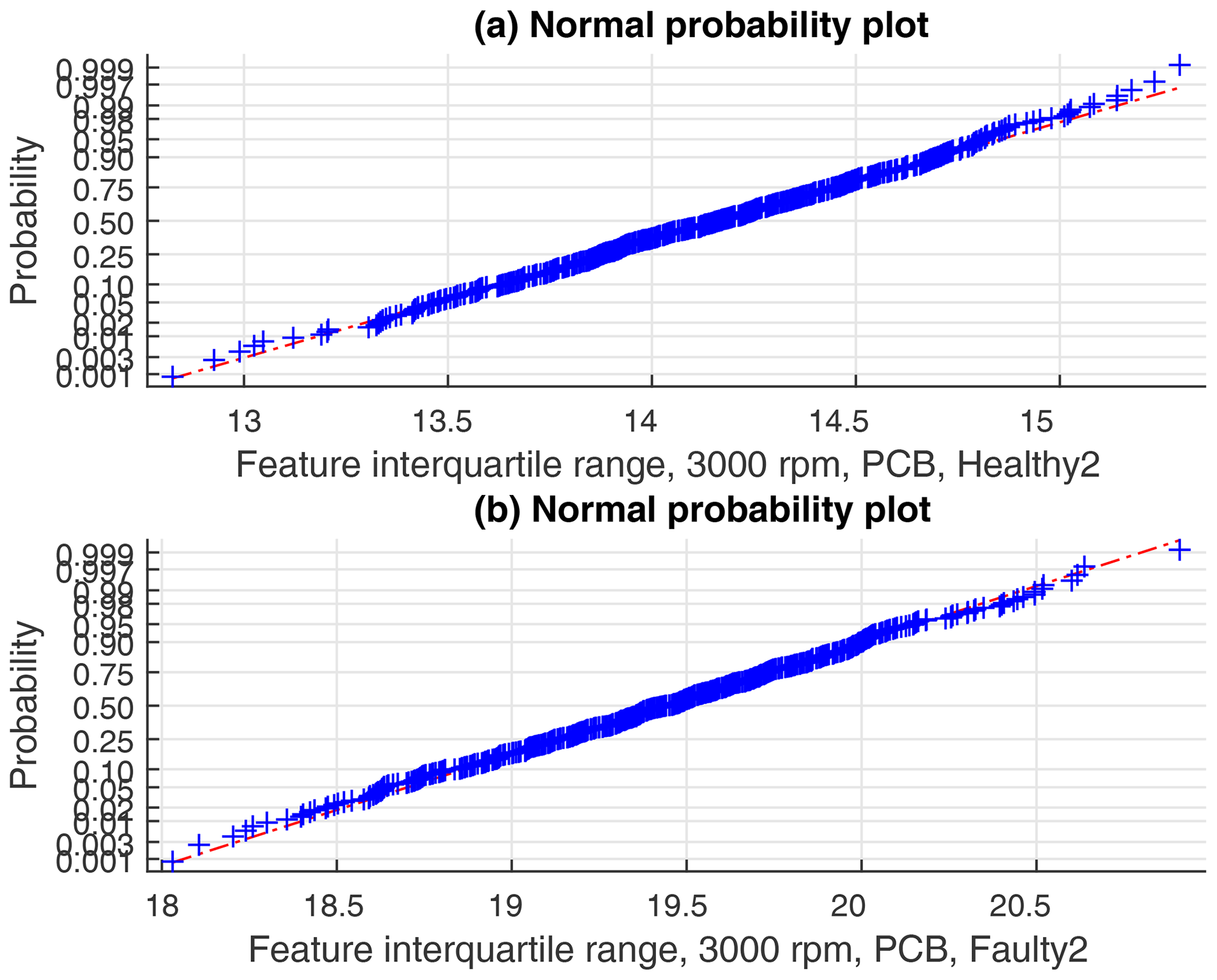
Figure 7 Normal probability plots of the feature interquartile range, 3000 rpm data, PCB sensor, and states Healthy2 and Faulty2.

The supervised-learning approach implies that the method depends on having a sufficient amount of annotated training data for all states (failure modes) to be monitored. There are also classifiers for one-class classification (also referred to as novelty detection) available (Tax, 2001). However, those techniques detect only a deviation from a nominal state and are thus prone to overdetection due to changing operation modes. Furthermore, the feature selection process depends on having an annotated dataset as well. For the ALT test no training data from different states were available; hence we used a novelty detection technique. For that purpose, the features selected in the gearbox test are observed by cumulative-sum (CUSUM) control charts (Hawkins and Olwell, 1998).

Given annotated training data, the whole process of feature extraction, feature selection and classification can be fully automated. The more useful the information in the training data is, the better the resulting feature subset and classifier are. In this context, information means different states, rotation speed, repeated measurements with different samples of the same bearing type and so on.

3.4 Evaluation of new data

The process of evaluating a new data sample is straightforward: the selected features are extracted in a sliding-window approach from the raw accelerometer signals, and the classifier is applied to those features. Since many classifiers are able to deliver class membership probabilities, it is generally also possible to determine instances lying between two distinct states. However, we restrict here the evaluation to crisp class decisions by detecting the maximum class probability for each observation.

If a set of new samples (i.e. the test dataset) contains the true class information (the ground truth), the estimated class can be compared to the ground truth to evaluate the quality of the classifier. For that purpose, many measures like accuracy, balanced accuracy, confusion matrices and receiver-operating-characteristic (ROC) curves are proposed in the literature (de Ridder et al., 2017).

4 Results

The results obtained by the proposed method are presented in this section. The accelerated lifetime test results are addressed first. This is followed by the results of the gearbox test.

4.1 Accelerated lifetime test

In the ALT test, the features were extracted from the raw accelerometer signals in an overlapping sliding-window approach (window length of 0.2 s and overlap of 0.1 s). That yields 199 observations per 20 s data batch. However, for final evaluation, only the mean value of those 199 observations of a data batch is observed. Unlike the gearbox setup, we had no data of different health states available for feature selection and classifier training in the accelerated lifetime test. Therefore we could not strictly follow the evaluation scheme proposed in Sect. 3. We were rather restricted to detect significant changes in the feature values. For that purpose, CUSUM control charts were applied to the behaviour of a feature over time. Due to the missing feature selection step, we evaluated the top-ranked features of the gearbox test. All of those features increased significantly towards the end of the test run for the 9.0 kN as well as for the 1.5 kN load conditions. For instance, feature 20 is depicted in Fig. 8. Due to the increasing feature value, the upper threshold of the CUSUM control chart is exceeded after approximately 7.3 h in the 9.0 kN case and 7.9 h in the 1.5 kN case, indicating a failure of the bearing. This result shows that the features identified in the gearbox test can be used to perform predictive maintenance of bearings by observing them using CUSUM control charts. For control purposes, Fig. 9 shows an arbitrarily chosen feature. The feature shows no significant trend, and the CUSUM control charts do not exceed the thresholds. This is a first indication that a wrongly chosen feature will no produce overdetections.

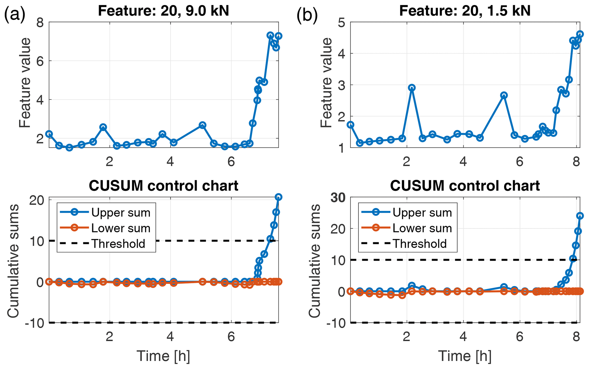
Figure 8 Feature values and CUSUM control charts for feature 20 in the ALT test for load 9.0 kN (a) and 1.5 kN (b).

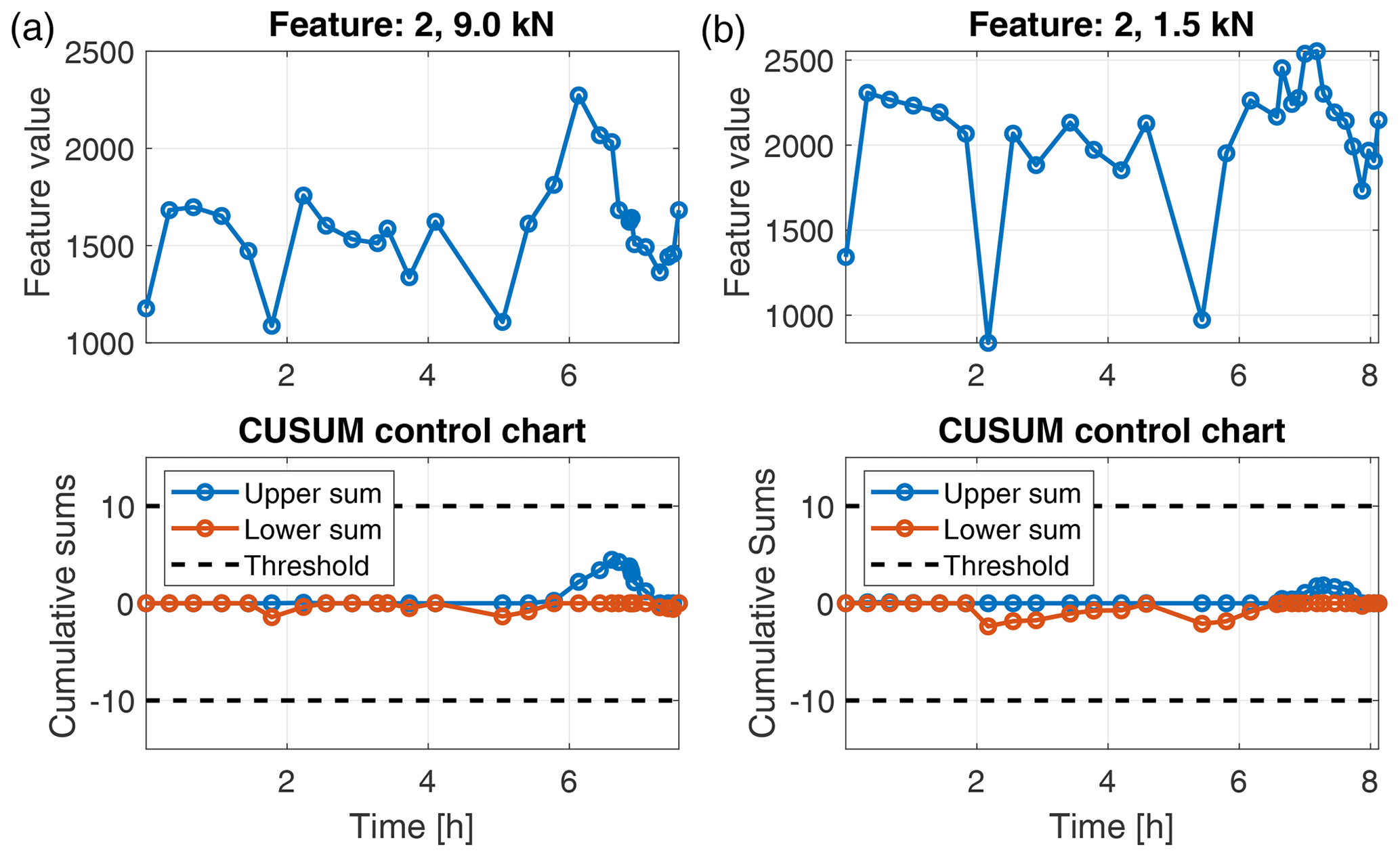
Figure 9 Feature values and CUSUM control charts for feature 2 in the ALT test for load 9.0 kN (a) and 1.5 kN (b).

4.2 Gearbox test

Just like in the ALT, the features for the gearbox test were extracted from the raw accelerometer signals in an overlapping sliding-window approach with a window length of 0.2 s and an overlap of 0.1 s, delivering again 199 observations for each 20 s data batch. After the extraction of all features, the feature selection algorithm was applied to the 3000 and 1500 rpm motor speed data independently. For feature selection, we did not use all available states. We used only the datasets of the states Healthy1, Healthy2 and Faulty2, but we did not use Indent and Faulty1. This procedure tests whether the method selects features that are suitable for the other two states as well or not. After feature selection, a quadratic-discriminant-analysis classifier, as described in Sect. 3.3, is trained in the space of the selected and annotated features. Only observations from the states Healthy2, Indent and Faulty2 are used for classifier training to test the generalizability of the proposed method. Moreover, for feature selection and classifier training, just two arbitrarily chosen data batches from each of the three states are used. That means that $\mathrm{199}\cdot \mathrm{2}\cdot \mathrm{3}=\mathrm{1194}$ observations were available for training. After training, validation was performed with another arbitrarily chosen 20 s data batch from all five bearing states, hence, $\mathrm{199}\cdot \mathrm{1}\cdot \mathrm{5}=\mathrm{995}$ observations. However, as the target class of the classifier we did not use those five states, but we only used the simplified states Healthy (containing Healthy1 and Healthy2), Indent and Faulty (containing Faulty1 and Faulty2). Since the states Healthy1 and Healthy2 and Faulty1 and Faulty2 are very similar, there is no reason to discriminate between them; in fact they are even supposed to produce similar feature values. As evaluation criteria, we use classification accuracy and the confusion matrix.

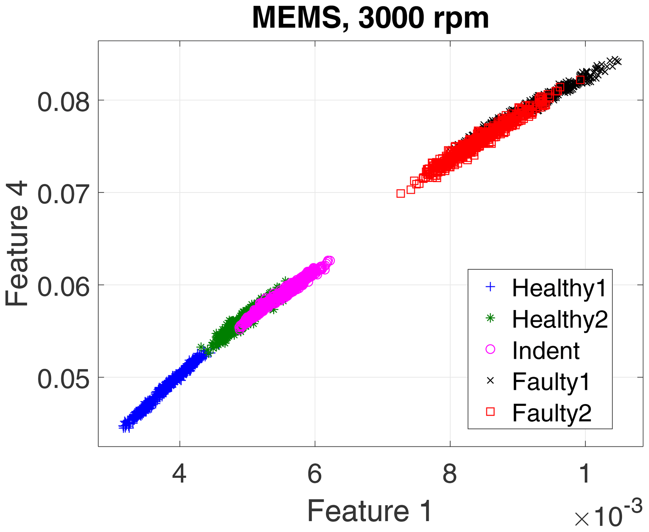
First, we evaluate the data of the high-end PCB accelerometer. For the 3000 rpm motor speed data, the algorithm selected three top-ranked features, and for the 1500 rpm data it selected four top-ranked features. However, for a first visual impression we show only the top two features for all recorded states and rotation speeds in a scatterplot in Fig. 10 (3000 rpm) and Fig. 11 (1500 rpm).

Figure 10 Scatterplot of top two features for the 3000 rpm PCB dataset.

Figure 11 Scatterplot of top two features for the 1500 rpm PCB dataset.

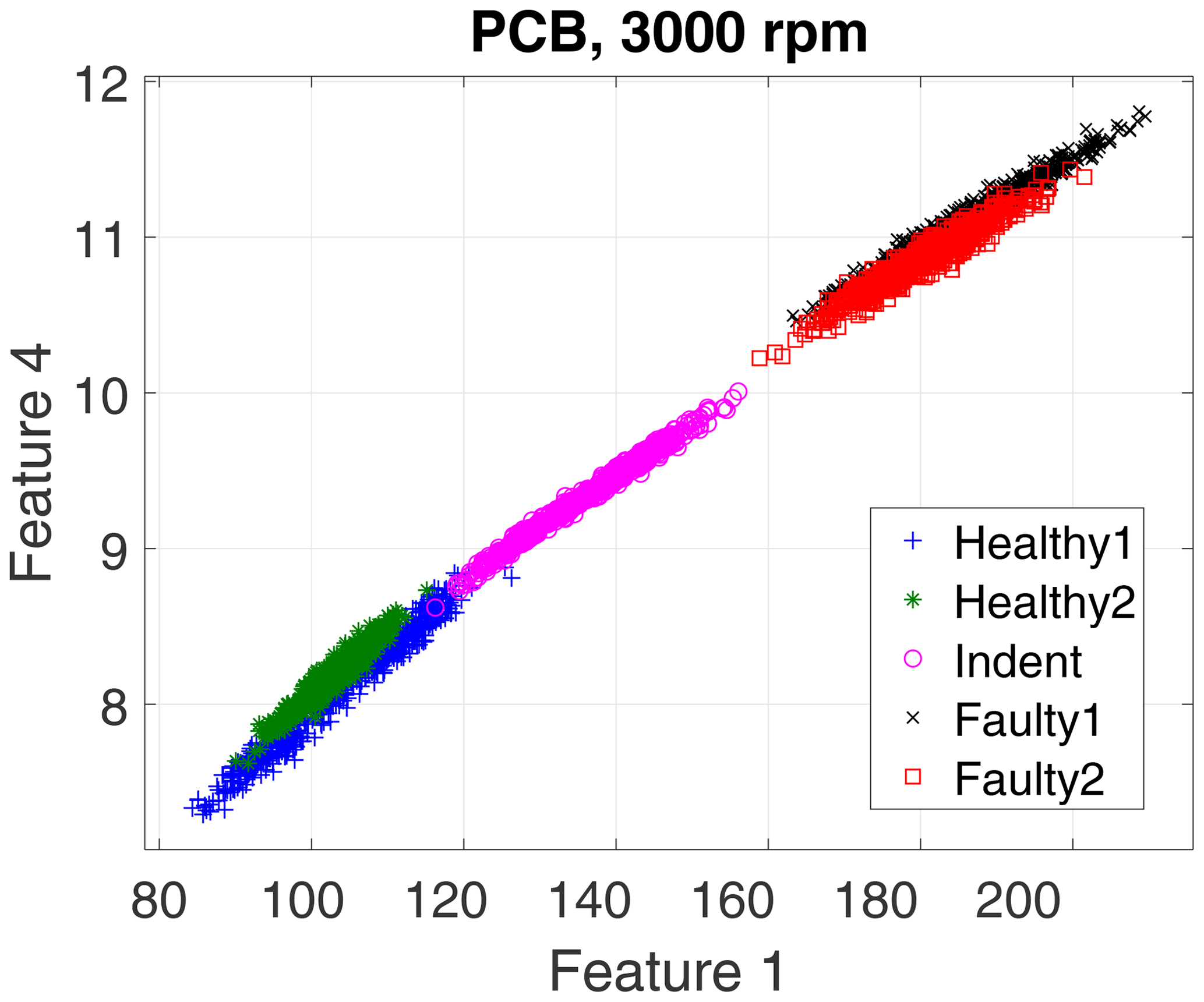
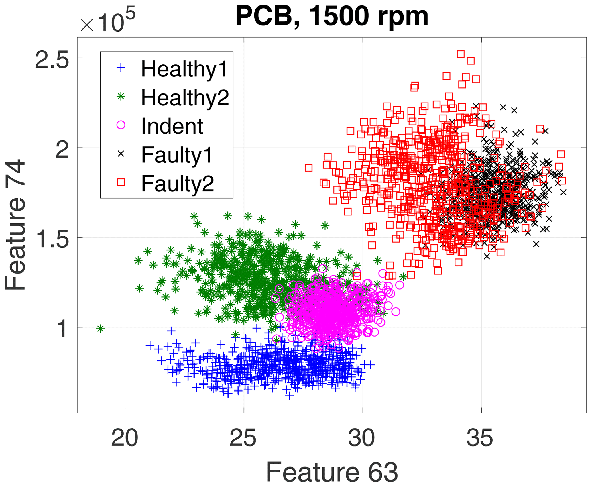
The scatterplots already indicate a few possible conclusions:

• Different top features were selected for the different rotation speeds.

• The 3000 rpm dataset revealed better separability.

• Faulty1 and Faulty2 produced similar feature values.

• In the 3000 rpm dataset, the Indent class lies somewhere in between the healthy and the faulty states.

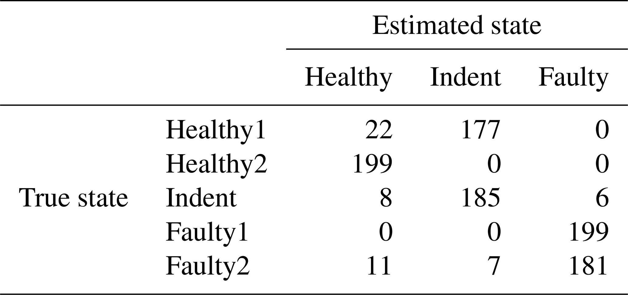
According to the feature selection step, the 3000 rpm data were validated with the top three features, and the 1500 rpm data were validated with the top four features. The validation yields 99.30 % accuracy for the 3000 rpm data (confusion matrix in Table 1) and 82.41 % accuracy (confusion matrix in Table 2) for the 1500 rpm data. That result confirms the first conclusion above: the separability of the states Healthy, Indent and Faulty in the 3000 rpm case is satisfying, while it is worse in the 1500 rpm case. Especially the state Healthy1 is misclassified in the 1500 rpm case. Since Healthy1 was not used for classifier training, it is obviously more likely to be misclassified.

Table 1 Confusion matrix for 3000 rpm PCB data and the top three features.

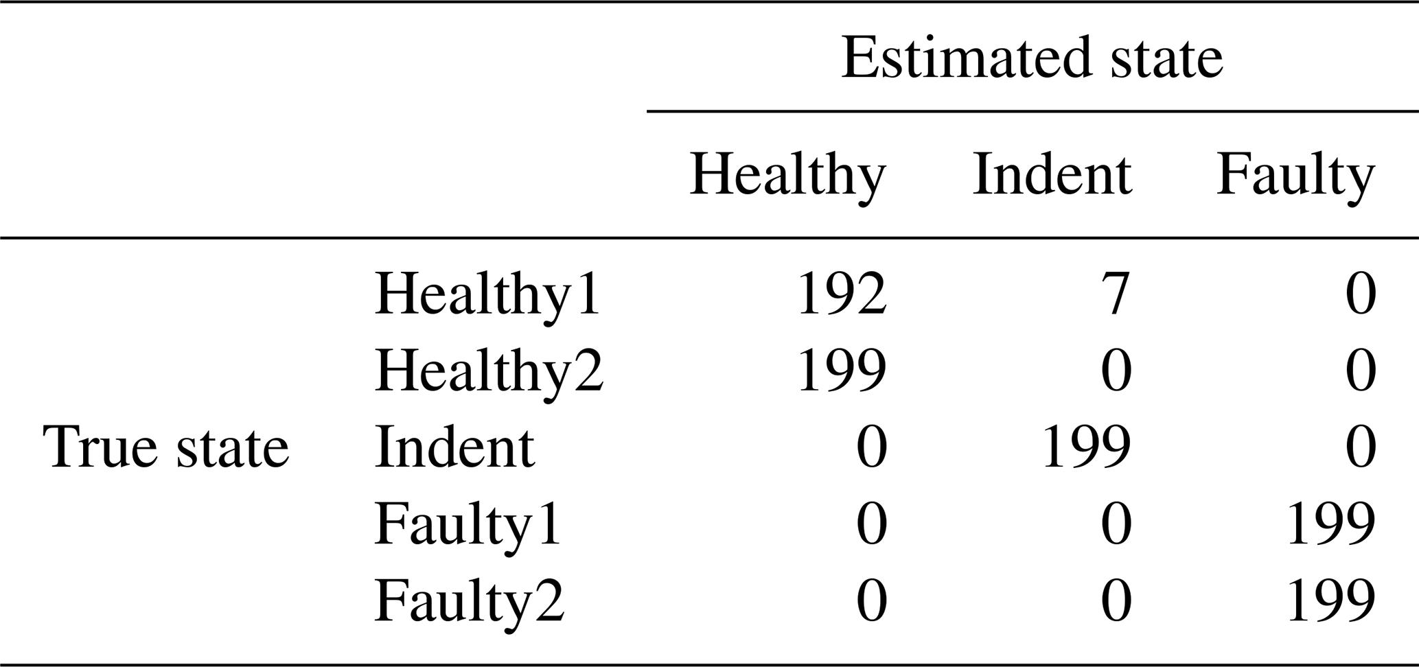
Table 2 Confusion matrix for 1500 rpm PCB data and the top four features.

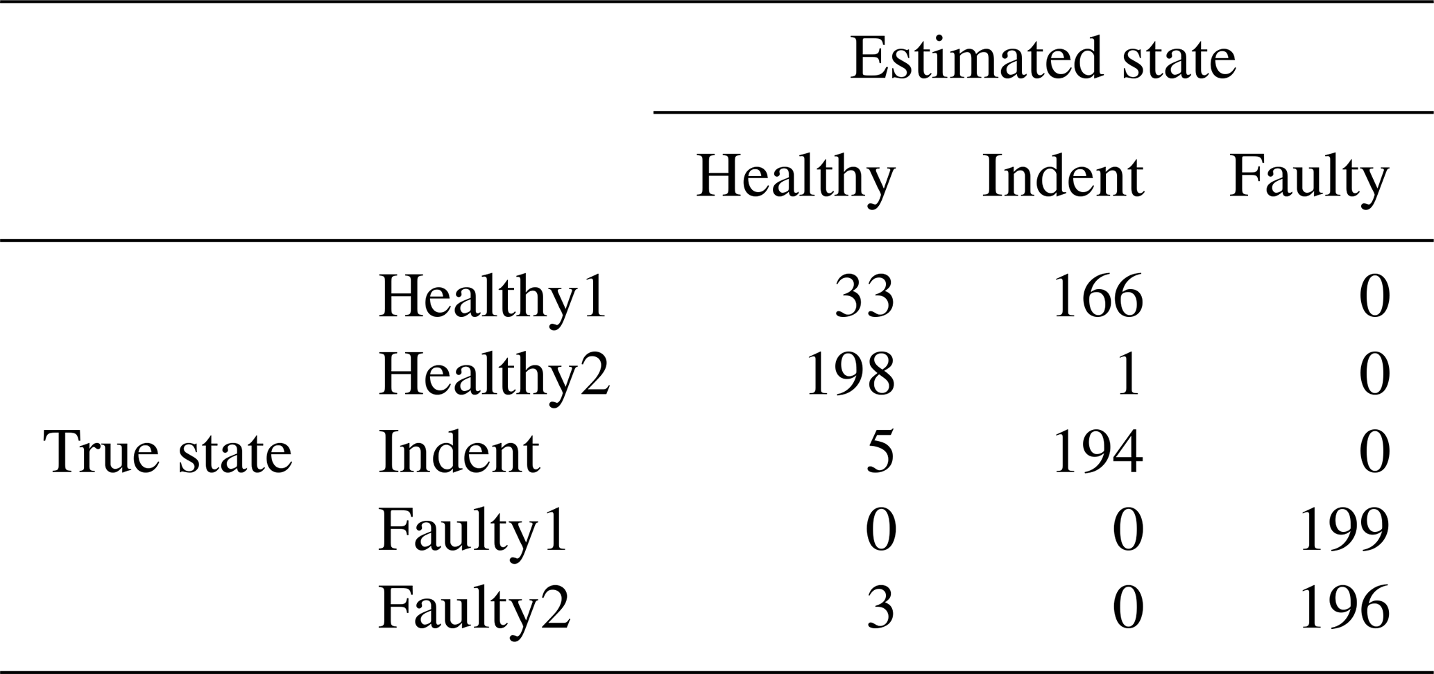
Table 3 Confusion matrix for 3000 rpm MEMS data and the top three features.

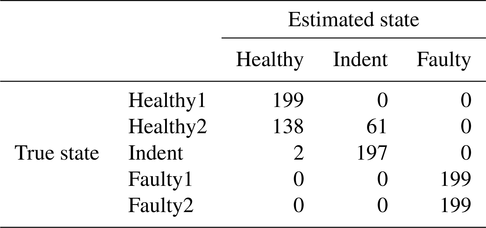
Table 4 Confusion matrix for 1500 rpm MEMS data and the top four features.

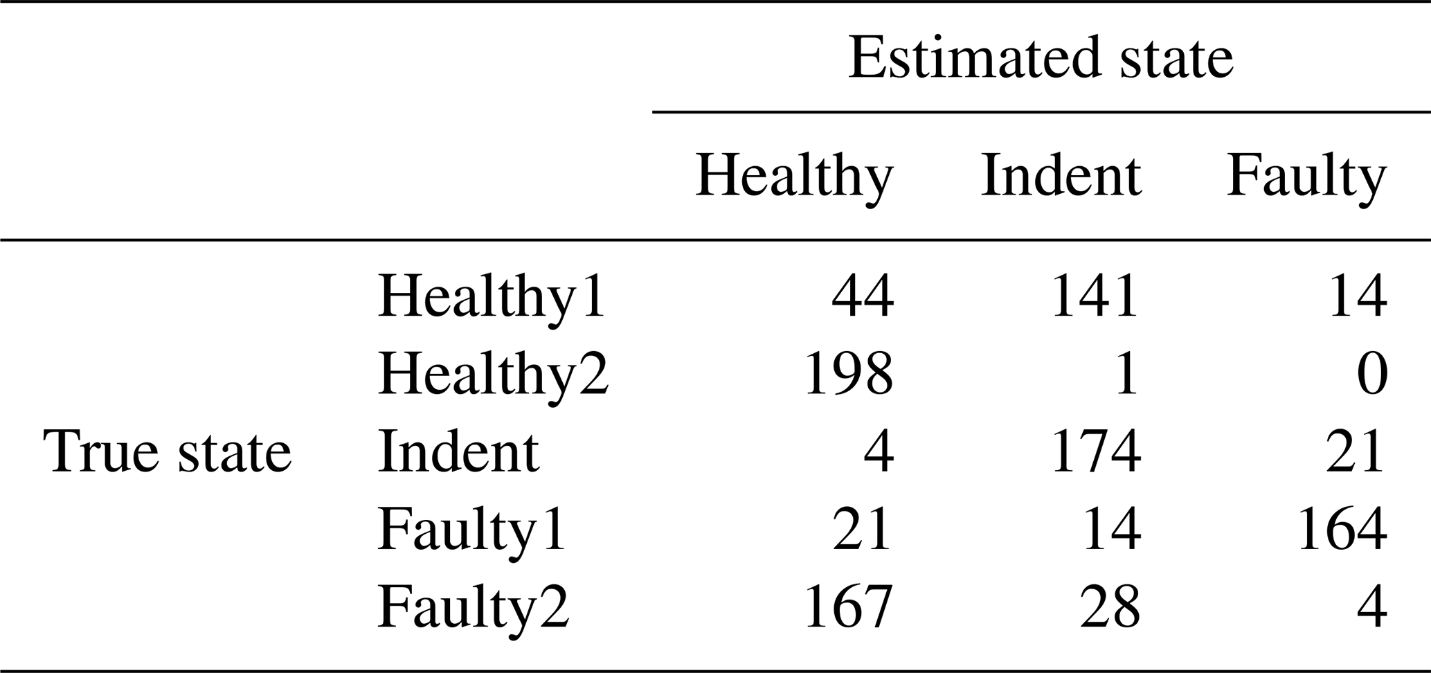
To compare the results of the PCB sensor with the MEMS sensor, we extracted the same features from the raw accelerometer data of the MEMS sensor and validated them in the same way. In the 3000 rpm case that yields 93.67 % accuracy (confusion matrix in Table 3; scatterplot of the top two features in Fig. 12), and in the 1500 rpm case that yields 78.99 % accuracy (confusion matrix in Table 4; the scatterplot of the top two features in Fig. 13). In both cases, the accuracy of the low-cost MEMS sensor data is lower than the accuracy of the high-end PCB sensor data. However, one might argue that the comparison is not fair, since the feature selection was performed with the PCB data. In our experiments, the MEMS sensor did not perform significantly better when the feature selection was performed using the MEMS data.

Figure 12 Scatterplot of top two features for the 3000 rpm MEMS dataset.

Figure 13 Scatterplot of top two features for the 1500 rpm MEMS dataset.

Since the effort for making steady-state speed measurements at every possible speed level is too high, it is desirable to have a less costly training data acquisition procedure. Therefore, we also tested the feasibility of using the ramp-up measurements for training a classifier. For that purpose, the target speed v_t rpm of the steady-state validation data is used to select a subset of the ramp-up data for classifier training. More specifically, we use the ramp-up data that represent a motor speed of $v=v_{\mathrm{t}}\pm \mathrm{20}$ rpm for training. With that data, the classifier is trained and applied to the steady-state validation data in the same way as described above. The accuracy values can be seen in Table 5, and the according confusion matrices are in Table 6 (3000 rpm PCB), Table 7 (3000 rpm MEMS), Table 8 (1500 rpm PCB) and Table 9 (1500 rpm MEMS). We see again that the high-end PCB sensor delivers better accuracy than the low-cost MEMS sensor. Moreover, a higher motor speed allows for more accurate classification than a lower motor speed. However, all accuracy values are too low for a reliable condition-monitoring system.

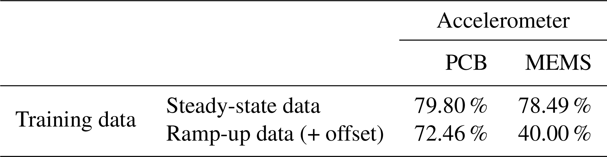
Table 5 Accuracy values for classifier training with ramp-up data.

Table 6 Confusion matrix for 3000 rpm PCB data and the top three features, classifier trained with ramp-up data.

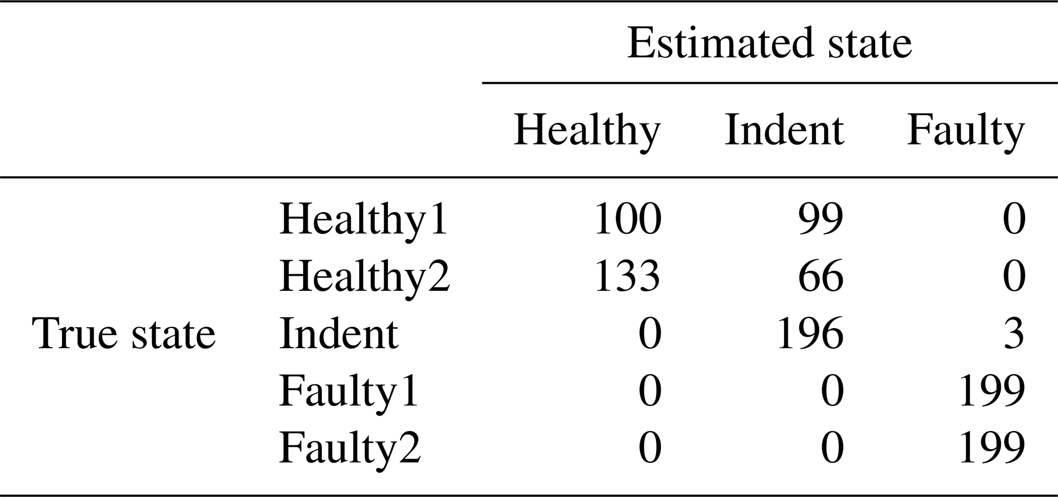
Table 7 Confusion matrix for 3000 rpm MEMS data and the top four features, classifier trained with ramp-up data.

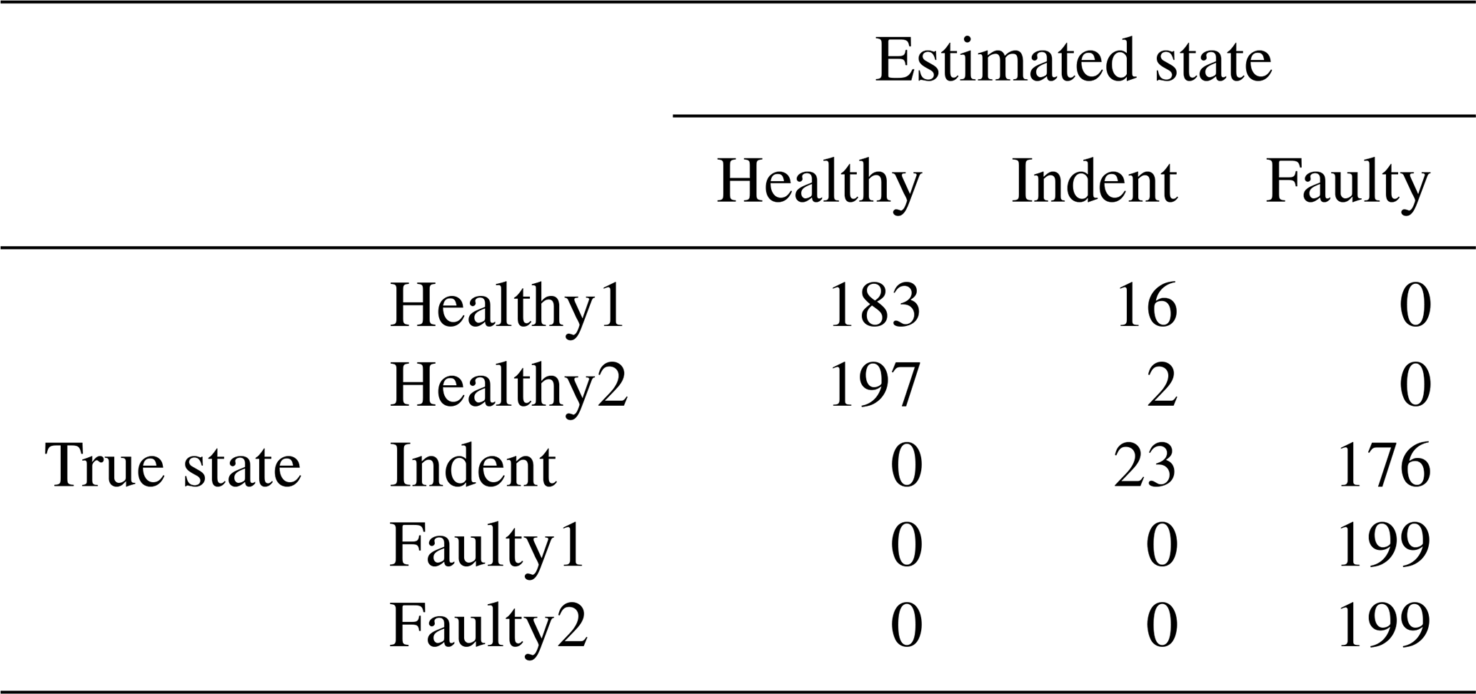
Table 8 Confusion matrix for 1500 rpm PCB data and the top three features, classifier trained with ramp-up data.

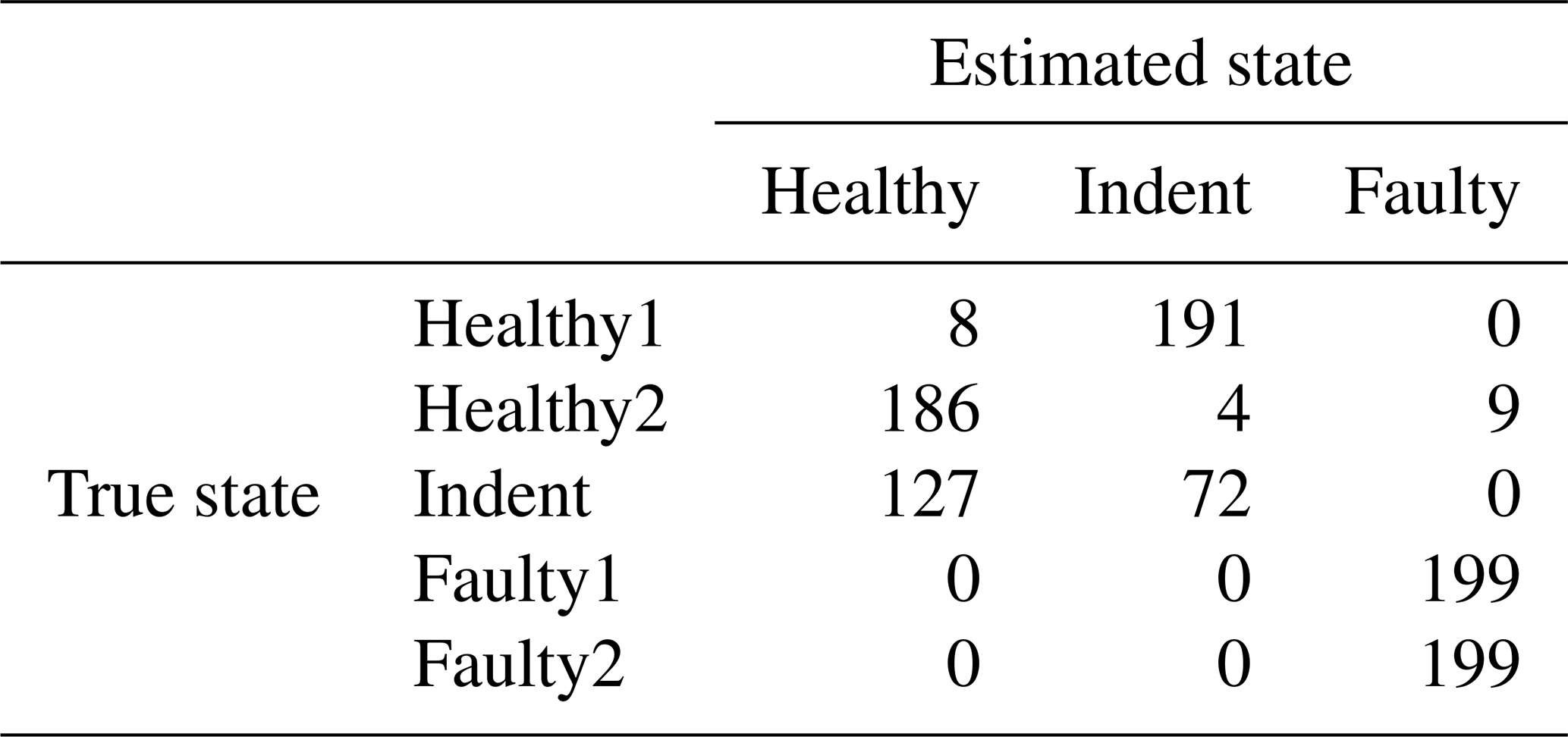
Table 9 Confusion matrix for 1500 rpm MEMS data and the top four features, classifier trained with ramp-up data.

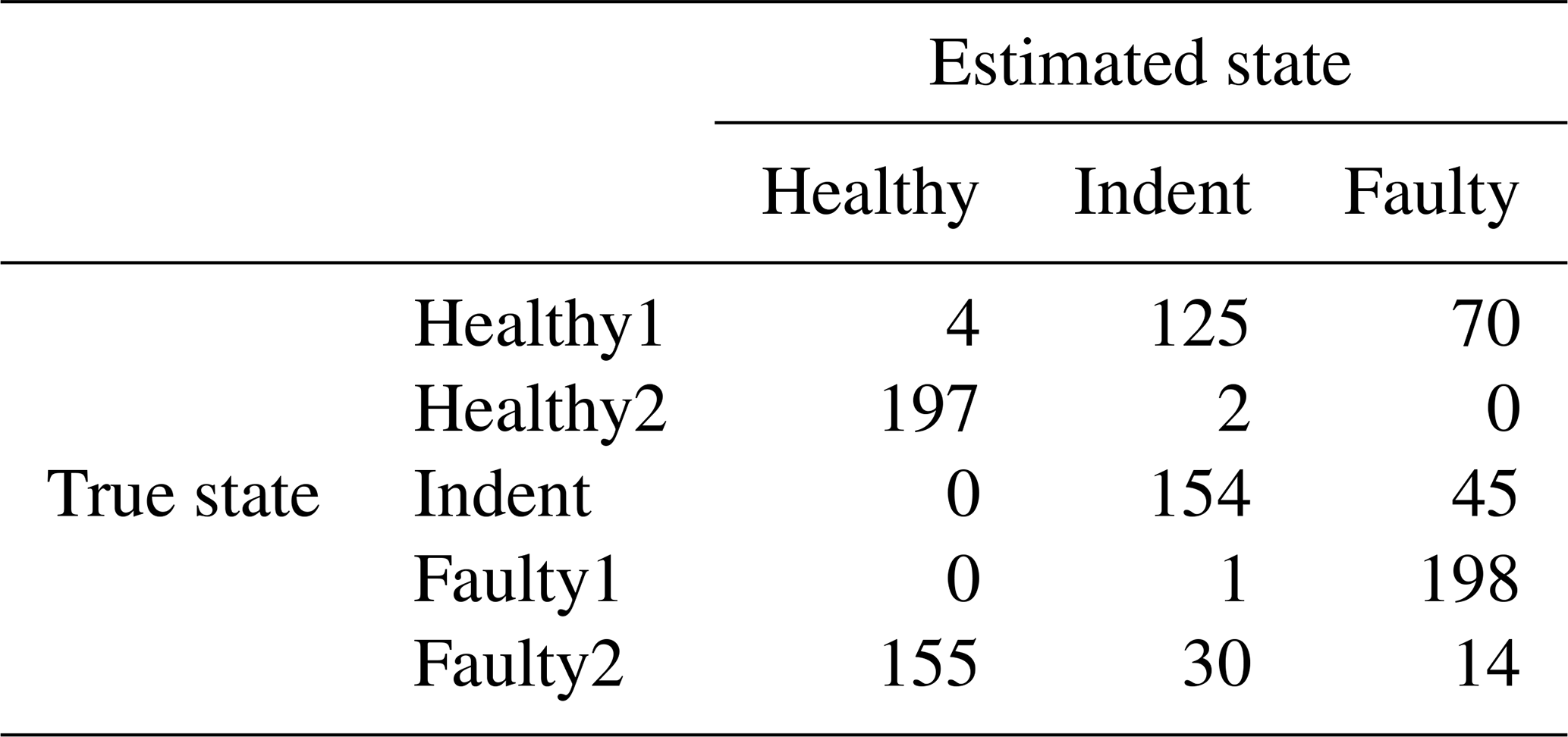
Interestingly, the accuracy increases significantly when an offset Θ is added to each dimension of the normalized feature space (normalizing each dimension of the feature space to μ=0 and σ=1 is a standard procedure in pattern recognition). For the PCB sensor data, an offset value of ${\mathrm{\Theta }}_{\mathrm{PCB}}=-\mathrm{0.25}$ is the best choice, while for the MEMS sensor data, an offset value of ${\mathrm{\Theta }}_{\mathrm{MEMS}}=-\mathrm{0.75}$ delivers the best results. The related accuracy values with the additional offsets can be seen in Table 10; the confusion matrices are found in Table 11 (3000 rpm PCB), Table 12 (3000 rpm MEMS data), Table 13 (1500 rpm PCB) and Table 14 (1500 rpm MEMS). In all cases, the accuracy increases by adding the offset to the normalized feature space. This fact might be due to dynamic effects of the ramp-up measurements; however, the exact reason will be the subject of further investigations of the data in the future. In this test, the same offset was added to all dimensions of the feature space. An individual offset for each dimension might further increase the accuracy. The offset was determined by a simple grid search approach using accuracy as the target value. For future applications it is desirable to find a way for a more sophisticated determination of an optimal offset.

Table 10 Accuracy values for classifier training with ramp-up data and additional offset.

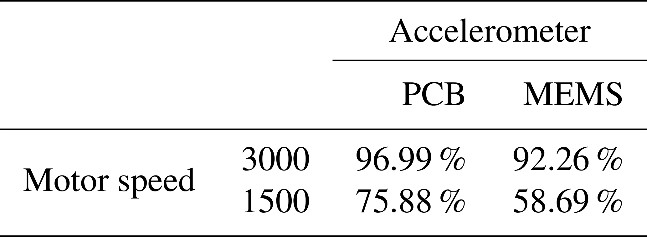
Table 11 Confusion matrix for 3000 rpm PCB data and the top three features, classifier trained with ramp-up data, with an additional offset in the steady-state validation data.

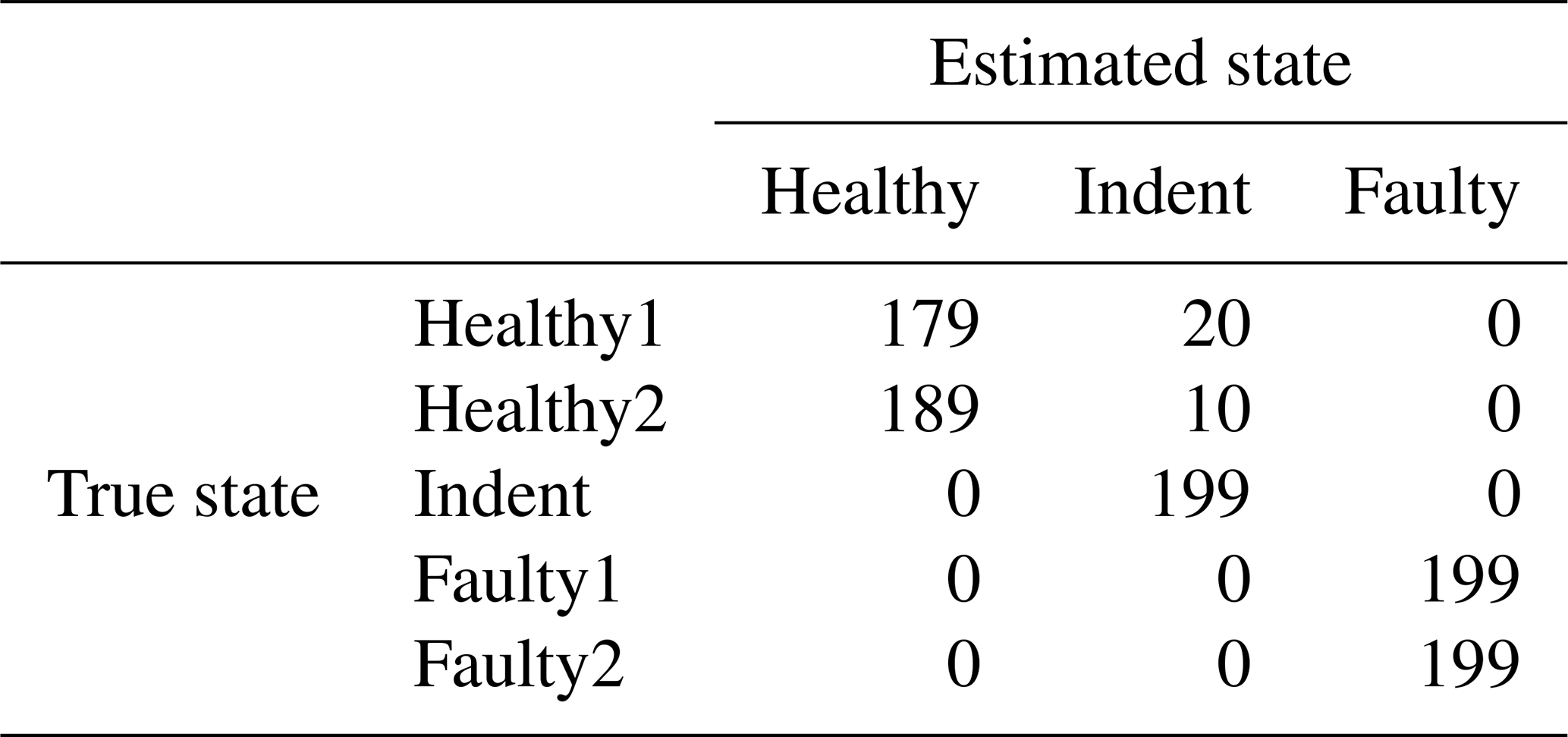
Table 12 Confusion matrix for 3000 rpm MEMS data and the top four features, classifier trained with ramp-up data, with an additional offset in the steady-state validation data.

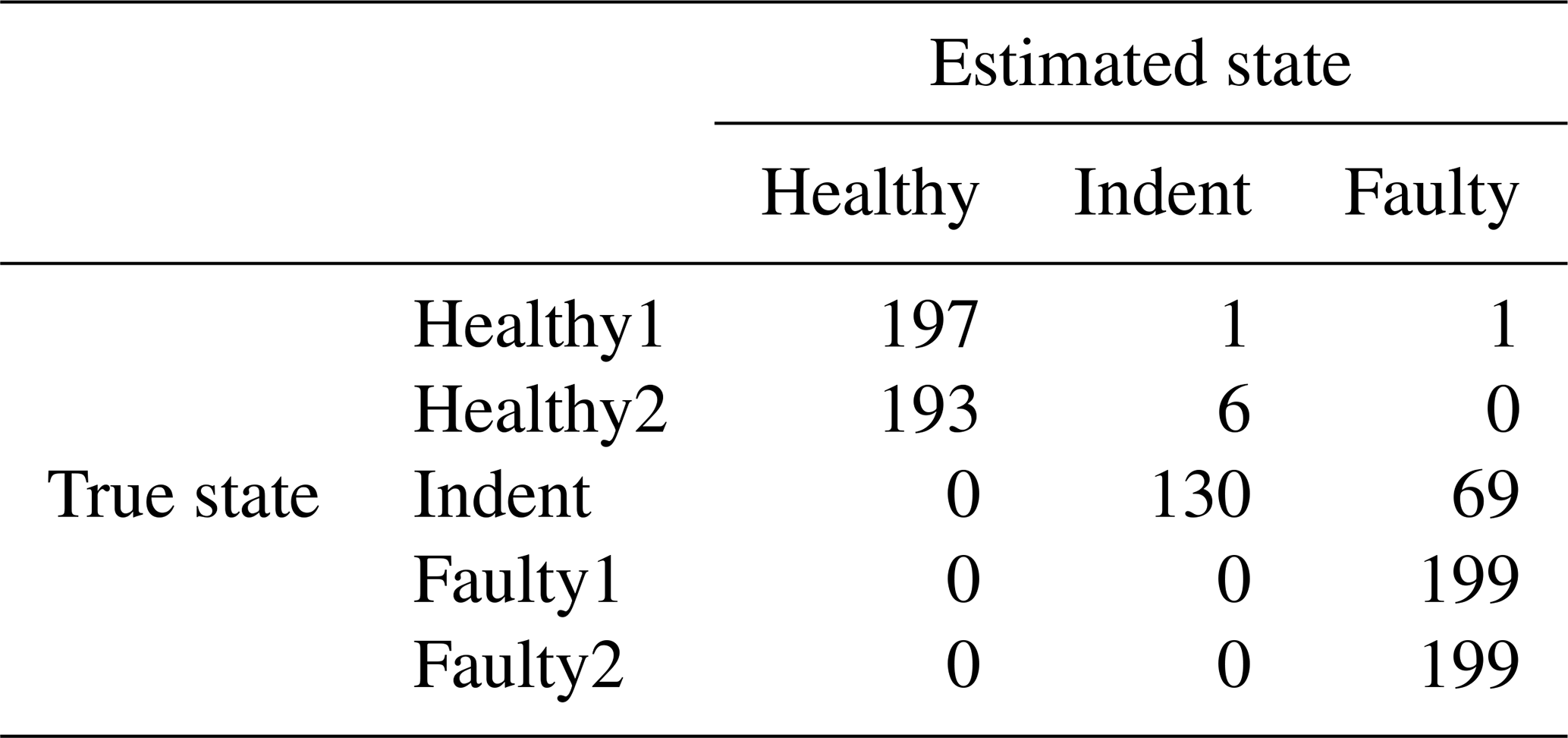
Table 13 Confusion matrix for 1500 rpm PCB data and the top three features, classifier trained with ramp-up data, with an additional offset in the steady-state validation data.

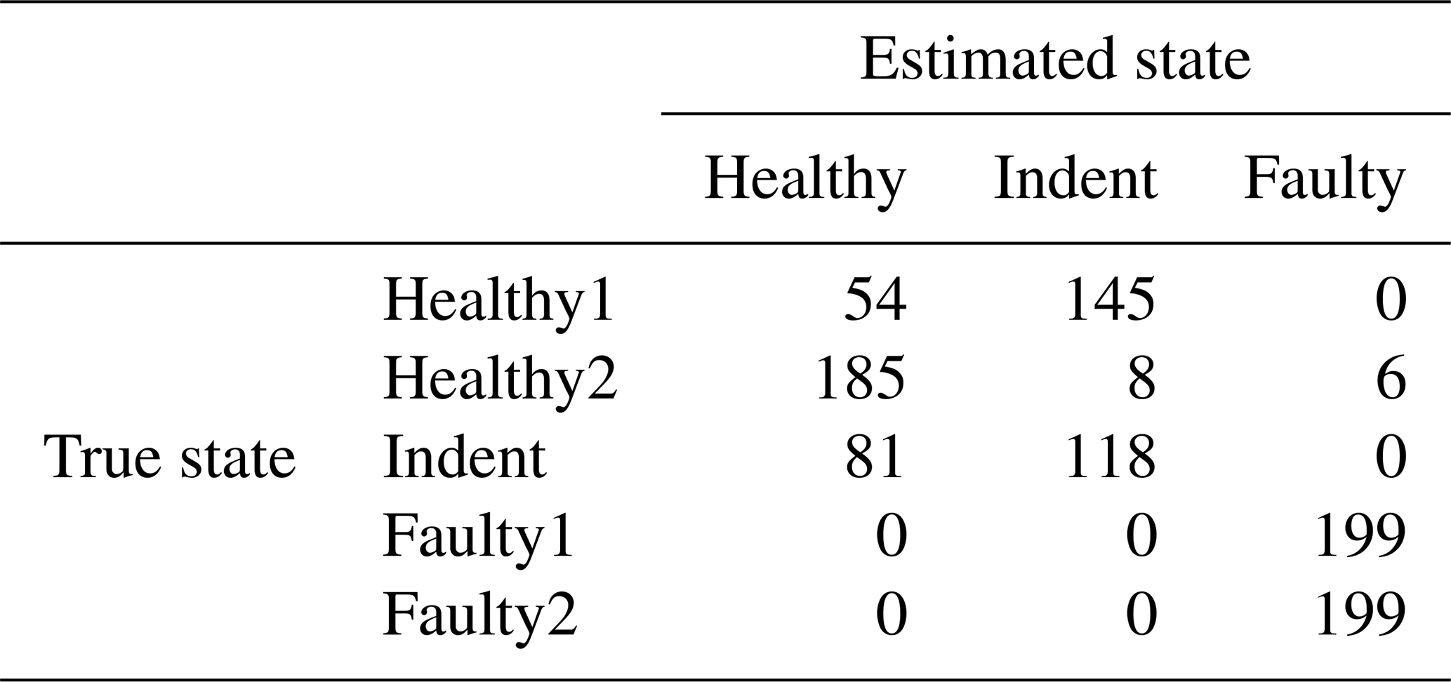
Table 14 Confusion matrix for 1500 rpm MEMS data and the top four features, classifier trained with ramp-up data, with an additional offset in the steady-state validation data.

As stated before, feature selection was performed for the 3000 rpm data and the 1500 rpm data separately. However, as stated in Sect. 1, it is desirable that the same feature set can be used for different revolution speeds to make the approach more universally applicable. Hence we also applied the features of the 3000 rpm data to the 1500 rpm data to assess the generalizability of those features. The resulting accuracy values for the test runs with steady-state and with ramp-up training data are shown in Table 15. In most cases (except the 1500 rpm MEMS data in the case of ramp-up training), the accuracy using the optimal feature set for 1500 rpm and the tested 3000 rpm feature set is rather similar. That implies that the 3000 rpm feature set is basically applicable to both cases. However, the accuracy values for the 1500 rpm case are too low for reliable bearing fault detection.

Table 15 Accuracy values for using the 3000 rpm feature set for the 1500 rpm data.

5 Conclusions

In this paper, we evaluate a previously proposed approach for the data-driven fault detection of bearings with regard to two main questions. Firstly, is it possible to train the proposed classifier even with non-steady-state measurements? Secondly, can the same feature sets be applied to different revolution speeds of the bearings? For that purpose, appropriate data have been acquired on a test bench and used for evaluation.

The results of this empirical study show that it is feasible to train the bearing fault diagnosis method with ramp-up data if the additional constant is added to the normalized feature space. The accuracy decrease is acceptable compared to steady-state training data, except for the case of the MEMS sensor and low revolution speed of 1500 rpm. A similar conclusion can be drawn regarding the other main goal of the paper. The 3000 rpm feature set performs acceptable even on the 1500 rpm data (compared to the 1500 rpm feature set). Again, the only exception is the 1500 rpm ramp-up data with the MEMS sensor, which delivers just the baseline accuracy. Overall, the accuracy of the 1500 rpm test is too low for a reliable fault diagnosis system.

Furthermore, it can be concluded that the classification accuracy increases with the higher rotational speed of the bearing, and the high-end PCB sensor allows for higher accuracy values than the low-cost MEMS sensor. Hence it is not possible to save costs by using less expensive sensors without accepting a ]significant decrease of detection accuracy.

The results of the ALT test show that an upcoming fault can be detected considerably before total failure of the bearing occurs. This leads to the conclusion that observing the selected features with CUSUM control charts is applicable for performing the predictive maintenance of bearings. In addition, a wrongly chosen feature does not lead to overdetections.

However, even though the results are promising, there are still investigations to be made. As mentioned before, the classifier can be trained with dynamic ramp-up data, and an additional offset in the normalized feature space allows for classification results that are almost as good as training with steady-state data. The exact reason for that offset will be topic of future analysis of the acquired data. The offset in the feature space was determined in a simple grid search approach. A more sophisticated choice of an optimal offset is desirable for the future. Moreover, we tested just two steady-state motor speeds. Further tests with more speeds will help to evaluate down to what speed the method delivers satisfying results and which features are best suited for different revolution speeds.