Compilation of training datasets for use of convolutional neural networks supporting automatic inspection processes in industry 4.0 based electronic manufacturing

Ensuring the highest quality standards at competitive prices is one of the greatest challenges in the manufacture of electronic products. The identification of flaws has the uppermost priority in the field of automotive electronics, particularly as a failure within this field can result in damages and fatalities. During assembling and soldering of printed circuit boards (PCBs) the circuit carriers can be subject to errors. Hence, automatic optical inspection (AOI) systems are used for real-time detection of visible flaws and defects in production.

This article introduces an application strategy for combining a deep learning concept with an optical inspection system based on image processing. Above all, the target is to reduce the risk of error slip through a second inspection. The concept is to have the inspection results additionally evaluated by a convolutional neural network. For this purpose, different training datasets for the deep learning procedures are examined and their effects on the classification accuracy for defect identification are assessed. Furthermore, a suitable compilation of image datasets is elaborated, which ensures the best possible error identification on solder joints of electrical assemblies. With the help of the results, convolutional neural networks can achieve a good recognition performance, so that these can support the automatic optical inspection in a profitable manner. Further research aims at integrating the concept in a fully automated way into the production process in order to decide on the product quality autonomously without human interference.

1 Introduction

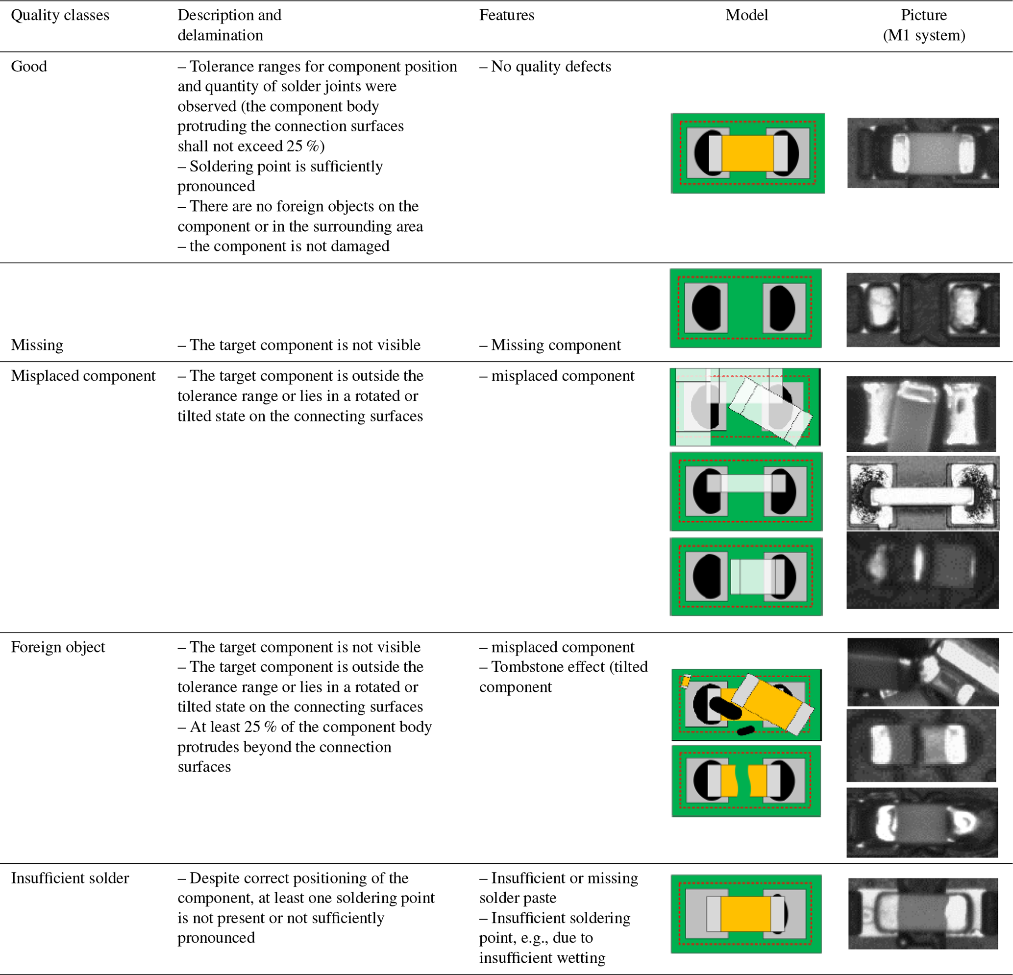
Electrical assemblies usually represent the core of electrical devices. Therefore, the manufacturing process of most electrical assemblies is fundamentally similar and is based on the assembly and soldering of components with a printed circuit board (PCB). Especially the quality of the solder joints between the component and the printed circuit board directly influences the durability and reliability of the products. During the assembly process, various flaws can occur on the components, the solder joints or the area surrounding the joints. Table 1 shows an overview of the possible defect patterns, their features and classification into quality classes (Berger, 2012).

Table 1 Definition of the quality classes of the chip component for the neural network (Berger, 2012).

In order to prevent further processing of defective assemblies, automatic optical inspection systems (AOIs) are integrated into the production lines as a non-invasive test method. An AOI system is usually equipped with several cameras and detects the defects using image-processing methods, such as local feature matching, morphological image comparison or blob detection. The circuit board is scanned for errors while the camera records an image of every component position. Thus, the prerequisite for the reliability of such a test is the complete visibility of the module subject to test. Due to technological change, a larger number of functions are being integrated into increasingly small installation spaces. Therefore, the rise in packing density means that solder joints can no longer be correctly identified, due to shadow effects or reflections from neighboring components. Consequently, the quality of the assemblies can no longer be adequately assessed as part of the optical inspection. This causes error slip and pseudo errors (non-genuine defects) in the test results. Another difficulty is based on the circumstances that the optical inspection can only determine the existence of defects but cannot recognize the exact type of error, such as a misplaced component. Hence, this problem results in the necessity to develop new automatic visual inspection systems. Therefore, there is a high demand for building an intelligent defect classification system to evaluate the assemblies from images of the inspection systems. The further development strategies include supporting the AOI system with deep learning to improve the accuracy of error check. The image capture of the solder joints needs to be evaluated once again with the help of a convolutional neural network (CNN) (Berger, 2012; Scheel, 1997).

The recognition performance of CNN is directly influenced by the composition of the training data. Nevertheless, literature research has shown that there is no uniform consensus in image preprocessing for the training of neural networks so far. Therefore, various approaches are available to balance the amount of training data within the classes (Frid-Adar et al., 2018; Roth et al., 2015; Zhang et al., 2019). In the context of the present work, the classification accuracy of the network is examined depending on different training datasets. For that reason, a suitable compilation of datasets is elaborated, which ensures the best possible error identification. Accordingly, various training datasets from original and artificially augmented images are developed. The purpose of this work is to determine which combination of training data is most suitable for the classification of an entire assembly.

2 Implementation of the network architecture

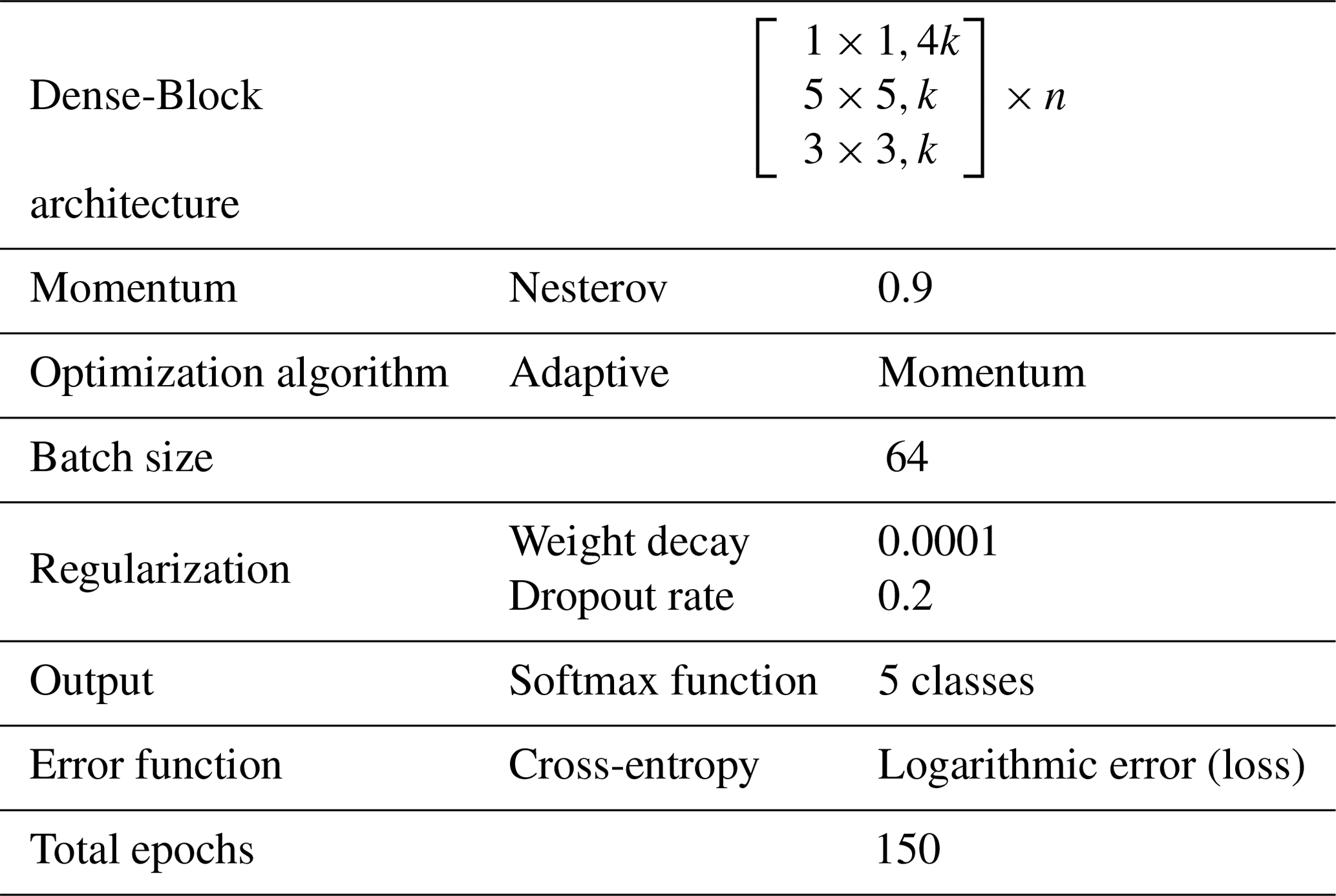
In preliminary investigations, various state-of-the-art image classification architectures are examined for their suitability with regard to the problem definition (He et al., 2015; Szegedy et al., 2014, 2016; Hu et al., 2017; Huang et al., 2018b). Therefore, the DenseNet architecture has proven to be the most suitable, due to the highest detection accuracy. The performance of DenseNet is highly attributed to the reuse of feature maps. Furthermore, all subsequent layers can access all feature maps learned by any of the layers (Huang et al., 2018a). In this study, a DenseNet with three Dense Blocks and two transition layers is used. Additionally, a 5×5 kernel to capture a larger value range is integrated into the Dense Blocks. The growth rate is set at k=24 and the three Dense Blocks have the configuration conditions n of $\mathrm{12}-\mathrm{24}-\mathrm{32}$. The training algorithm is the momentum optimizer with Nesterov momentum. The variables for the hyperparameters Nesterov momentum m=0.9, dropout rate d=0.2 and weight decay $w_{\mathrm{d}}={\mathrm{10}}^{-\mathrm{4}}$ were chosen according to the original publication and were adopted unchanged (Huang et al., 2018a). The initial learning rate is set to α=0.01 and is decreased by a factor of 10 every 50 epochs. In order to prevent the training progress from stagnating, the learning rate is reduced by a factor of f=0.94 if there is no decrease in error after 10 epochs (Szegedy et al., 2016). Furthermore, cross-entropy is used as the error function. At the end of the network, a fully connected layer of 1000 neurons connects the network with the Softmax classifier and the initial weights are initialized with random values. All experiments run for 150 epochs, using a batch size of 64 images. The CNN training is based on four graphical processing units (GPUs) of type PClex 16 NVIDIA TITAN V with 5120 Cuda-Cores, a clock rate of 1455 MHz and a frame buffer of 12 GB. The network is implemented in the Python programming language with the Tensorflow deep learning library. Table 2 below shows the software settings and implementation details for training the CNN.

Table 2 Implementation details of the used DenseNet version.

3 Presentation and selection of training data

The shortage of training data is mostly a limiting factor for the training of neural networks. Therefore, the main issue often lies in generating balanced datasets. In industrial practice, the datasets are usually obtained from production. The aim of quality assurance is to deliver products that meet the highest quality standards. Accordingly, there are often only a few images or small image data sizes of faulty assemblies available. In addition, some types of defects occur more frequently than others, for manufacturing reasons. The aim is to work out a suitable compilation of a training dataset for the classification of quality states of electrical assemblies, which fulfils the requirements in industrial applications. Consequently, surface-mounted chip components of different sizes are used for the investigations, which are represented by capacitors and resistors. For chip components, one letter and four digits define the designation of the component type. The letter indicates the component type (R for resistor, C for capacitor), while the first two digits denote the case length between the pins and the last two digits describe the width of the component. The unit is normally indicated in 1∕100 inch. Figure 1 provides an overview of the used components.

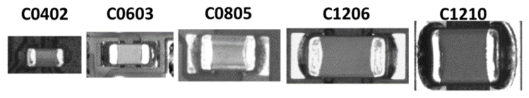
Figure 1 Overview of the capacitors (chip components) used as image recording of an M1 inspection system.

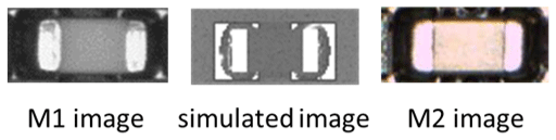
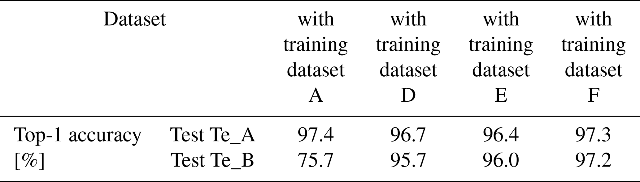
All images used in this study were taken by optical inspection systems from different manufacturers. In an anonymous form, the respective images are referred to below as “Manufacturer M1” or “Manufacturer M2”. Depending on the inspection system, grayscale or color images are captured (refer to Fig. 2). Accordingly, the network is trained with each of seven different datasets (refer to Table 3). The model with the lowest validation error during the training is selected and tested on six test datasets. These test datasets come from different sources and show various component types (refer to Table 3). In this article a concept is worked out, which is applicable to all component types. Besides, it is determined whether a global training dataset can be used or a separate model has to be trained for each component. In addition, a cross-plant or cross-line application is being examined. Test images are all original and unmodified. This way, it would be possible to integrate neural networks into the real production process to support optical quality assurance.

Figure 2 Overview of used image types.

Table 3 Overview of used datasets.

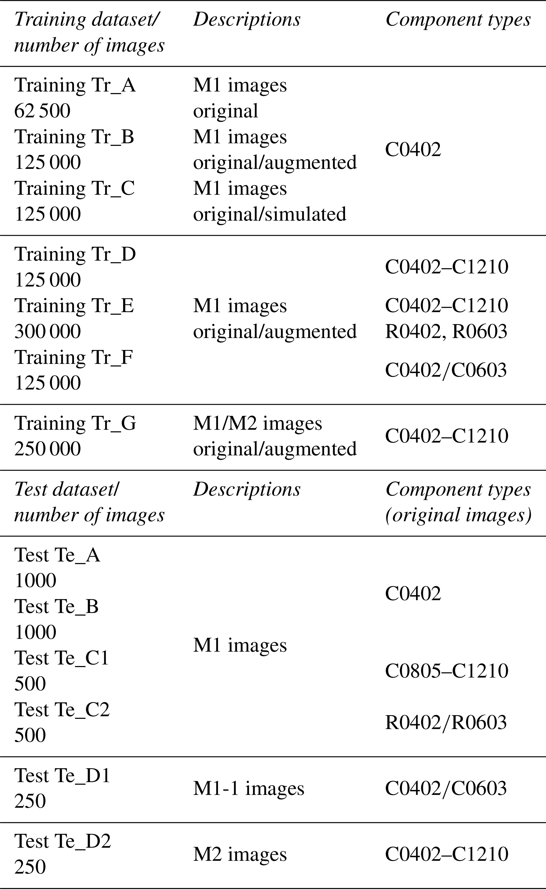
Test dataset Te_A contains images of capacitor C0402 captured by the inspection system of manufacturer M1. Most of the errors occur at this relatively small component, due to its size. As a result, most training data are available for C0402. Therefore, this dataset is used to evaluate the recognition of the individual quality classes in particular. Test datasets Te_B (C0603) and Te_C1 (C0805–C1210) contain larger capacitors, while resistors (R0402, R0603) are represented in test dataset Te_C2. Thus, these data are used to check whether the trained network can also be applied to unknown component types. Additionally, test dataset Te_D1 includes images captured by another M1 optical inspection system (M1-1) whose images are not part of the training data. For test dataset Te_D2, data from another inspection system of manufacturer M2 are used. It is examined whether the performance of the network is coupled to the camera module of the training data. The test datasets have 200, 100 or 50 test images per class. Since the test data must exclusively consist of original data, the dataset size is partly limited by the occurrence of errors in production. The exact composition and size of the datasets can be seen in Table 3. Since both grayscale images and color images are generated depending on the system, there are different dimensions with regard to the depth channel. For this reason, all images are fed into the network in three channels, which leads to an expansion of the input volume of the grayscale images. The size of the input is $\mathrm{120}\times \mathrm{120}\times \mathrm{3}\times \mathrm{8}$ bit for all datasets.

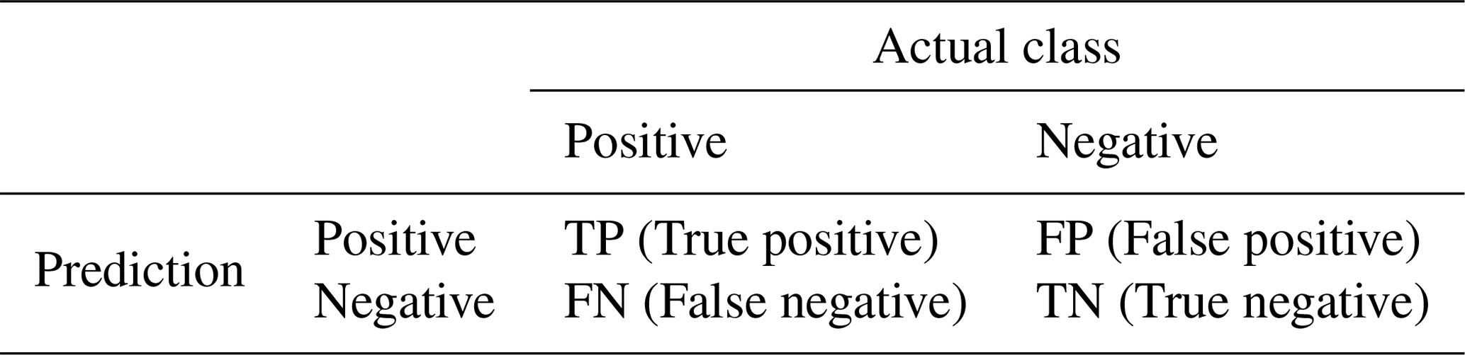
To compare the effects of the individual training datasets, uniform evaluation metrics are required. In industry, accuracy is one of the most important measurement parameters for evaluating an optical inspection system. Hence, the accuracy metric is used to measure the recognition performance of the CNN in an interpretable way (refer to Eq. 1). The accuracy of a neural network is usually calculated in the form of a percentage and is the measure of how accurate the model predictions are compared to the true data. Therefore, this intuitive metric is used below for a first, preliminary assessment. Based on further evaluation metrics, the detection performance of the individual classes can be assessed more accurately. In this context, a confusion matrix can be used to compare the classification results of the neural network with the actual classes (refer to Table 4). The precision shows (refer to Eq. 2) how many of the classes predicted to be positive are actually positive, while the recall indicates how many positive target expenditures are covered by the positive predictions (refer to Eq. 3). Since neither of the values provides a general statement, the combination is used to calculate the F1-Score. With the F1-Score (refer to Eq. 4), the recognition accuracy of each class can be assessed individually (Raschka and Mirjalili, 2018).

$$\begin{array}{}\text{(1)}& {\displaystyle }& {\displaystyle }\mathrm{Accuracy}={\displaystyle \frac{\mathrm{TP}+\mathrm{TN}}{\mathrm{TP}+\mathrm{TN}+\mathrm{FP}+\mathrm{FN}}}\text{(2)}& {\displaystyle }& {\displaystyle }\mathrm{Precision}={\displaystyle \frac{\mathrm{TP}}{\mathrm{TP}+\mathrm{FP}}}\text{(3)}& {\displaystyle }& {\displaystyle }\mathrm{Recall}={\displaystyle \frac{\mathrm{TP}}{\mathrm{TP}+\mathrm{FN}}}\text{(4)}& {\displaystyle }& {\displaystyle }\mathrm{F}{\mathrm{1}}_{\mathrm{Score}}=\mathrm{2}\cdot {\displaystyle \frac{\mathrm{Precision}\cdot \mathrm{Recall}}{\mathrm{Precision}+\mathrm{Recall}}}\end{array}$$

Table 4 Confusion matrix.

3.1 Component-homogenous training datasets

In the first instance, it has to be examined whether a component-homogeneous training dataset can be used to inspect an entire assembly. A component-heterogeneous dataset consists only of one component type. This would allow merely one model to be applied in each production line to classify the entire assemblies. Therefore, the classification accuracy is examined with three different training datasets. Each of the datasets contains the same basic data but is extended by different methods. Consequently, all training datasets contain exceptionally images of capacitor C0402, which were taken by the M1 inspection systems and are available as grayscale images. The data are collected from 15 different production lines at two manufacturing locations. Capacitor C0402 is a small component, whose features are difficult to extract because of its size. In case of high classification precision, the approach of C0402 can easily be applied to any other larger component.

Training dataset Tr_A consists exclusively of unchanged original inspection images and therefore is taken as a basic dataset and reference. Each class has 12 500 images, resulting in a total training dataset of 62 500. During the training, 2500 randomly selected images are used for validation. Training datasets Tr_B and Tr_C define an expanded version of training dataset Tr_A. Accordingly, for the generation of training dataset Tr_B, the basic dataset Tr_A is used and augmented to 125 000 images (25 000 per class) to double the data stock. A current practice for image data augmentation is to perform geometric and color variations (Perez and Wang, 2017; Shorten and Khoshgoftaar, 2019). In this work, rotations and translations were used to create geometric changes. The filtering techniques histogram equalization, various gamma filters, the Gaussian Blue filter and the artificial generation of noise were applied to change the color palette of the images. In this context, the influence of data size and diversity through the augmentation has to be examined. Training dataset Tr_C is doubled by adding simulated images to the basic dataset Tr_A. While the augmentation is based on a copy of the original images, a higher variance within the classes shall be created by simulation. The simulated images are not taken by an optical inspection system, but are artificially generated training data (refer to Fig. 2).

As depicted in Fig. 3 the performance of the network is most efficient for all training datasets on test dataset Te_A of C0402. Accordingly, there is a similarity between all training datasets in their general classification accuracy, with training dataset Tr_C achieving a maximum overall recognition performance of 97.6 %. Based on all datasets being component-homogeneous by the same component type, the network is able to focus specifically on this capacitor.

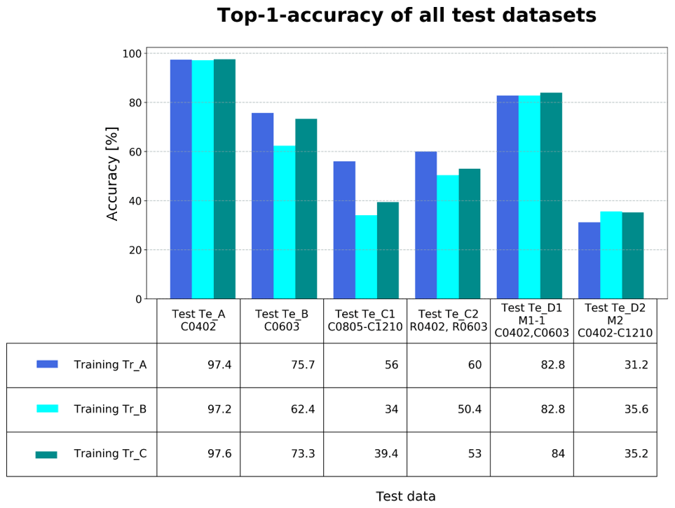
Figure 3 Top-1 accuracy of all test datasets with the homogeneous training datasets Tr_A, Tr_B, and Tr_C.

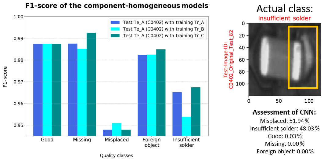
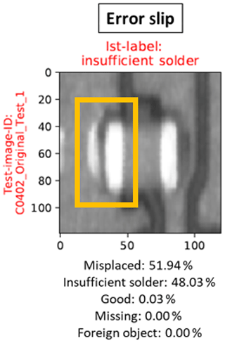
Figure 4 Classification results of test dataset Te_A with the homogeneous training datasets and prediction result of a misplaced C0402.

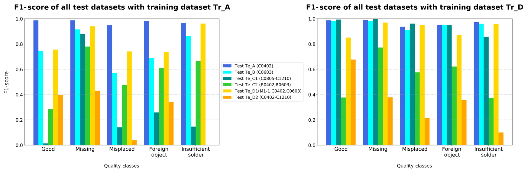
While the evaluation metrics (refer to Fig. 4) for the categories “Good”, “Missing” and “Foreign Object” of test dataset Tr_A indicate a comparatively good detection performance, the other two classes can be less well identified by the network – regardless of the training dataset. It can be particularly noted that class “Misplaced” has higher misclassifications for all test datasets (refer to Fig. 5). The F1-Score values at “Misplaced” and “Insufficient Solder” show that the two classes are often incorrectly predicted. Additionally, the low values at “Misplaced” indicate that other categories are frequently erroneously assigned to this class. In this context some defect scenarios – especially the incorrect placement of components – often occur in combination with other errors, and the network is able to recognize the feature correlation (refer to Fig. 4). This leads to the assumption that a misplaced component makes it difficult to classify the correct state of quality and that the dominant feature seems to influence the decision of the network. Since there is no component offset in classes “Good” and “Missing”, these categories are more clearly defined and have a comparatively higher recognition accuracy.

Figure 5 Error slip on C0402 of test dataset Te_A.

Failure type “Missing” has the highest detection accuracy regardless of the component type or the inspection system. The reason is that this failure type can be identified independently of the component. Due to the absence of the components, there are less complex features. It is noticeable that the addition of the simulated images has positive effects on the classification performance of this category compared to the other training datasets (refer to Fig. 4). Consequently, the simulated data adjust the network weights so that class “Missing” can be recognized independently of the component type or picture source.

The biggest challenge of quality assurance is to identify defective products. Besides, incorrectly valued non-defective products lead to unnecessary additional costs. For this reason, the behavior of the network with regard to error slip and pseudo errors must be considered more closely (refer to Table 5). The error slip is very low in all test data, which is probably due to the characteristics of class “Good”. The central component of this category differs more from the other classes: few erroneous test data classify it as “Good”. Usually the error slip can be observed at joints whose quality lies in the limit range of tolerance. Figure 5 shows a correctly placed component, whose left leg is not sufficiently pronounced. The component and its solder joints are assessed as functional, due to the dominant “Good” features, although defects on the left solder joint site can already be identified. A similar behavior can be observed with the pseudo errors. Therefore, the test datasets with larger components have particularly more pseudo-error rates. The components unknown to the network are often assigned to category “Foreign Object” regardless of their quality state, so that there is an increased pseudo-error occurrence (see Fig. 6).

Table 5 Error slip of the network on test dataset Te_A.

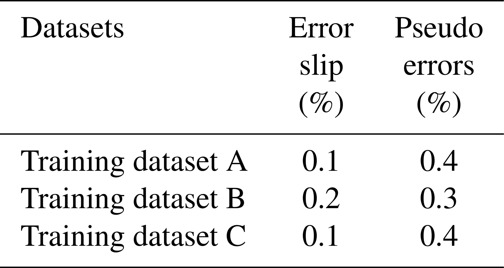
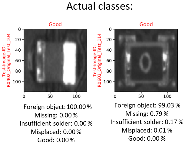
Figure 6 Classification results of resistors (test dataset Te_C2) with training dataset Tr_A.

While the quality classes of C0402 are comparatively well recognized, the recognition performance decreases with increasing component size (see Fig. 3). This is particularly evident from the low-accuracy score values for test datasets Te_B and Te_C1. It is remarkable that both the larger chip components and the resistors of the same size in test dataset Te_C2 are primarily identified as “Foreign Object” (refer to Fig. 6). The reason for this behavior is probably the unknown or larger manifestations of the components, since the network is primarily adjusted to the smaller C0402. The models trained with the extended training datasets Tr_B and Tr_C show less favorable results on test datasets Te_B, Te_C1 and Te_C2. It is anticipated that the additional data expansions are adjusting the weights of the network towards to the smaller C0402, whereby the quality states of the larger components will be recognized with more difficulty. Only recognition accuracies of test datasets Te_D1 and Te_D2 show similar results.

Compared to the capacitors, there are different types of chip resistors with regard to the component body. The resistors have an enhanced edged shape of body and some have additional imprints on their backs (see Fig. 6). While one type of resistor clearly resembles the capacitors in appearance (see Fig. 6 left), the other types of resistor have different features (see Fig. 6 right). For this reason, it should be investigated to what extent the component body type influences the detection performance of the network despite the same component size. Based on the results of test dataset Te_C2 it is obvious that especially the object shape plays an important role in the classification. Despite the same component size (C/R0402, C/R0603) the network models cannot correctly assign the quality states of the resistors. Since the assessment depends on all visible features and outward-facing surfaces, the network cannot make correct decisions for these component types, due to the lack of information. During the placement process, the C0402 is overlaid by larger components, due to occasional misplacements. This constellation is assigned to class “Foreign Object” in the training data. Due to the associated weight adjustment, the network tends to identify unknown or larger components as contaminations. Regardless of the component type, the image recordings of other AOI systems (test datasets Te_D1 and Te_D2), whose images are not part of the training data, are increasingly assigned to class “Foreign Object”. Furthermore, the metrics of test dataset Te_D1 show (refer to Fig. 3) that poor performance is achieved despite the identical inspection system from the same manufacturer. In this case, machine-specific influences such as deviating illumination conditions or camera noise change the representation of the relevant features. The lack of robustness of neural networks against noise effects has already been observed (Tang and Eliasmith, 2010). If there is insufficient image information for identification, the affected test image is classified to category “Foreign Object”.

It can be concluded that the augmentation and simulation of the training data have not led to a better recognition performance in terms of test dataset Te_A with the same component type. The reason may be that the augmentation increases the number of images, but not the information content of the images. Therefore, the augmentation only generates a modified copy of the original images, while the variance and manifestations of the individual quality classes are not increased. The simulated images of components and solder joints are only idealized scenarios. This means that the relevant features are not sufficiently or realistically represented to improve the network performance. Consequently, augmentation or simulating data should only be used if fewer training data are available or if there is an underrepresentation of individual classes. In view of the problem, this approach did not improve the detection performance overall.

Considering the results, a component-homogeneous training dataset cannot be used to inspect an entire assembly with components of different geometrical shapes and sizes. Unknown components cannot be classified correctly despite the same geometry and equivalent features of the quality classes. Therefore, the network not only extracts the bare characteristics of a failure type, but rather adjusts its weights according to the size distances and surface characteristics of the respective component. For this reason, a greater variance of training data by different component types is recommended for further investigations.

3.2 Component-heterogeneous training datasets

The previous chapter has shown that component-homogeneous training datasets are not suitable for the analysis of an entire assembly. For this reason, it should be investigated whether a component-heterogeneous dataset can be used to classify components of different sizes. For this purpose, two different training datasets diversely in the composition of the component types are examined.

Training dataset Tr_D (125 000 images) contains M1 images of capacitors C0402, C0603, C0805, C1206 and C1210. For each class 5000 images per component are used. The model trained with dataset Tr_D will be used for further retraining with different components to investigate whether it is possible to retrain the network without starting the training process again from the beginning. As new components, resistors (R) R0402 and R0603 are added to dataset Tr_D with 5000 images per quality class to generate training dataset Tr_E (Tr_D + R). Based on test dataset Te_C2, the success of the retraining will be evaluated subsequently. Since the frequency of defects decreases as the size of the components increases, the representation of the original data per class is determined by the occurrence of the respective failure type. Due to wider electrical connection surfaces, the error type “Insufficient Solder” occurs less frequently with larger components. For this reason, incomplete data are enriched by augmenting them to generate a balanced training dataset.

The results of the F1-Score metrics for training dataset Tr_D (especially on test datasets Te_B and Te_C1) show that the network can also recognize the quality states of the larger components C0603–C1210 (Fig. 7). Due to the higher variance of the component types, the classification performance of the larger capacitors of test datasets Te_B, Te_C1 and Te_D1 can be increased. In particular, the prominent classes “Good” and “Missing” are easily identified for all components. Consequently, the expansion of the training dataset leads to more complex kernels and made it possible to adjust the weights to all different chip components (Raschka and Mirjalili, 2018; Müller and Guido, 2017). The prerequisite for the recognition of the component and the quality class seems to depend on a component's presence in the training dataset. In this context, there is no difference in the classification performance between the individual components. By increasing the intra-class variance, the network can be tuned more accurately to classify different components (Wei et al., 2015).

Figure 7 F1-Score of all test datasets with training datasets Tr_A and Tr_D.

As has already been observed for training dataset Tr_A, the components cannot be classified correctly in the images taken by other inspection systems. This is illustrated by the weak F1-Score results (Fig. 7) of test datasets Te_D1 and Te_D2. Nevertheless, the actual recognition accuracy of test dataset Te_D1 compared to training dataset A could be increased. This effect is attributed to the high data variance of training dataset Tr_D. Besides, the increased data variance probably diminishes a camera-dependent adjustment of the network weights.

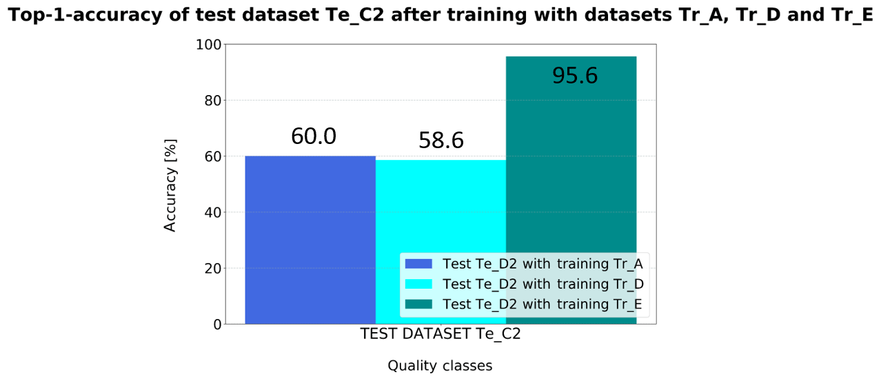
Training with dataset Tr_E enables the resistors to be recognized. This is due to the fact that the accuracy is substantially increased on test dataset Te_C2 compared to previous training datasets (refer to Fig. 8). Therefore, the retrained network is able to classify newly learned components. The retraining process seems to bring about an additional adjustment of the weights, so that the quality status of new components can be classified. The results have shown that with a high variety in the training dataset different components can be inspected.

Figure 8 Detection accuracy on the resistors depending on the different training datasets.

However, with increasing variance in different components in the training dataset, a slight decrease in the recognition performance is also observed in the individual component types (refer to Table 6). It is assumed that, due to the large variety of data, the network weights are in favor of all components, which have an adverse effect on the identification of the individual component. To investigate whether a trade-off between variance and detection performance can be found, training dataset Tr_F is exclusively composed of two capacitors of adjacent sizes. The aim is to benefit from the small difference in size or the similarity between components C0402 and C0603. For each class 12 500 M1 images per capacitor are available. Classes “Foreign Object” and “Insufficient Solder” of C0603 are enriched by augmentation, due to a slight deficit of these error types.

Table 6 Overview of the Top-1 accuracy depending on the data variance.

Although the component variance was increased, no losses of classification accuracy of test dataset Te_A can be observed in comparison to the homogeneous training datasets. Therefore, the expansion of dataset Tr_F has a particularly positive effect on the recognition performance of C0603. With training dataset Tr_F, comparable classification accuracies can be achieved for both component types C0402 and C0603 (Fig. 9). In this context, it is assumed that the small size difference of the capacitors enables an increased favorable adjustment of the filter weights for both components. The other test datasets have similar recognition results to the classification by the model trained with dataset Tr_A (refer to Fig. 3). This is probably due to the similarity of the two capacitors in the training dataset.

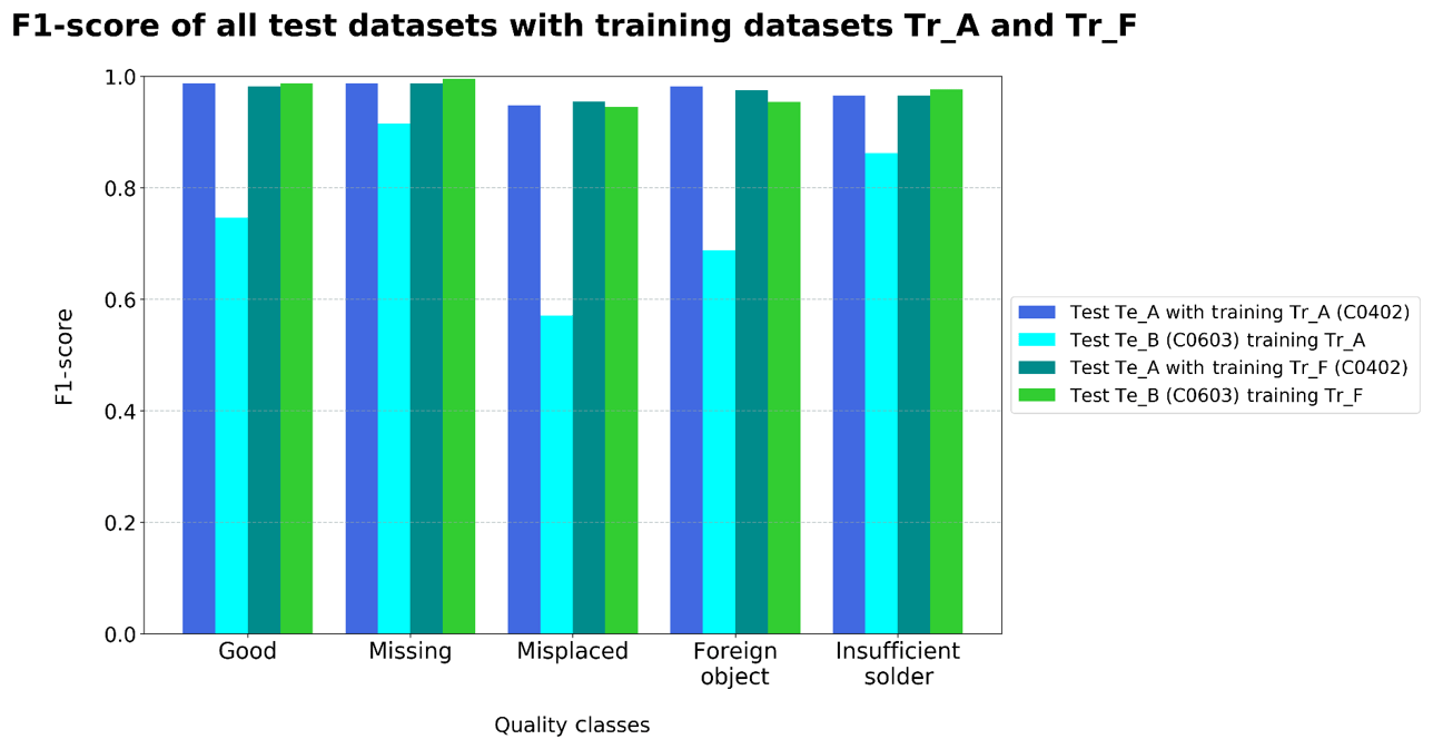
Figure 9 F1-Score on capacitors C0402 and C0603 depending on the different training datasets.

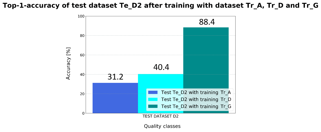
Figure 10 Detection accuracy on test dataset Te_D2 depending on the different training datasets.

Based on these results, it is assumed that the presence of the respective component size or component shape in the training datasets plays an important role in the recognition performance of the CNN. The quality classes are therefore taught in relation to size and appearance of the respective component. It is appropriate to use components of similar sizes to increase the variance or information content in the training data. Due to the comparatively small differences in size, the filter weights could be adapted better to the capacitors. In this way, a recognition performance comparable to that of the homogeneous training datasets can be achieved without a loss of classification accuracy in the individual component. For this reason, an increase in recognition accuracy could be reached compared to the training with datasets Tr_D and Tr_E (Wei et al., 2015).

3.3 Combination of training datasets from different inspection systems

In the following segment it will be examined whether a CNN can also be used across inspection systems. For this reason, the training dataset Tr_G is generated as an extension of the training dataset Tr_D to ensure a classification of images from different inspection systems. In order to meet this challenge, the training dataset Tr_G consists of the data from two types of AOI machines. Training dataset Tr_D of the M1 inspection systems served as the basic dataset, which is doubled by the addition of images of the M2 AOI type (50 000 images per class). Each capacitor (C0402, C0603, C0805, C1206 and C1210) is represented by 10 000 images per class (5000 images from each AOI system). Therefore, both component types as well as the images from the two inspection machine types M1 and M2 are available as a balanced dataset for each class. The images by M1 only show the assemblies in grayscale, whereas M2 produces three-channel color images (refer to Fig. 2). Due to a lack of data, the M2 images are partly augmented.

The expansion of the training data by adding the M2 images has a direct effect on the detection performance in classifying test dataset Te_D2 (Fig. 10). The results of the general accuracy show that mixed training datasets can compensate the recognition problem with images from other inspection systems. Error slippage and pseudo errors in particular are reduced. Due to the greater variance in the training dataset, more complex network kernels are generated for better classification of images from different sources (Wei et al., 2015). Besides, the heterogeneous data constellation prevents a camera-dependent adjustment of the network weights, which means the CNN can be used across different AOI systems.

It can be summarized that the results for test datasets Te_A–D1 are similar to those obtained with training datasets Tr_D and Tr_E. Nevertheless, the total misclassification rates of all test datasets with training dataset Tr_G are slightly higher than the rate of basic dataset Tr_D. The constellation of the network weights based on the additional M2 data has been adjusted in such a way that it has an adverse effect on the identification performance of the individual component types. However, the error slip of test datasets Te_A and Te_D1 could be minimized to zero. This effect is caused by the high variance of training dataset G. In particular, the concise classes “Good” and “Missing” are recognized well for all tested data. Nevertheless, the classes with an additional misplaced component were still poorly identified. Due to their different object geometry the resistors in dataset Te_C2 are difficult to classify even by this model and are highly likely to be assigned to the class “Foreign Object”.

The comparatively high recognition performance on test dataset Te_A is due to the high number of original data from C0402 in this training dataset. As fewer errors occur in production with increasing component size, fewer original image data are available for these components. Besides, fewer images could be obtained with the M2 AOI. By augmenting, the dataset can be increased, but not the variability of the individual quality classes. Because of the higher intra-class variance, due to the high proportion of original images, the training of the network can be improved with respect to C0402 or the images of the M1 inspection system.

4 Conclusion

The main aim of this research is to provide solutions for problems in the manufacturing industry. The major focus is on the generation of training datasets that can achieve a good recognition performance for the quality classes of the different components. It is particularly important to avoid error slippage and pseudo errors, so that the automatic optical inspection systems can be supported in the best possible way. Error slippage and pseudo errors occur more frequently if the component type to be evaluated is not represented in the training data or the image material was taken by an external inspection system. The results show that a trained model can be used across production lines or plants, provided that the training dataset contains images from the local inspection system. In this context, a single model can realize an inspection of different components as long as all component types to be evaluated are represented in the training dataset. If available, original images should be preferred over augmented data because the results show a connection between higher recognition performance and an increasing proportion of original data. Especially, original images have the advantage that they can represent the greatest variance and forms of features within the classes. Enrichment of the dataset by augmentation or simulation can be used for smaller or unbalanced datasets. It is observed that with increasing heterogeneity of the training dataset the recognition performance of the individual components decreases. A separate model does not have to be created for each component; it has proven to be effective to combine components of the same shape but different sizes into one training dataset or network model.