Calibrating a high-speed contact-resonance profilometer

A European EMPIR project, which aims to use large-scale, 5 mm × 200 µm × 50 µm ($L\times W\times H$), piezoresistive microprobes for contact resonance applications, a well-established measurement mode of atomic force microscopes (AFMs), is being funded. As the probes used in this project are much larger in size than typical AFM probes, however, some of the simplifications and assumptions made for AFM probes are not applicable.

This study presents a guide on how to systematically create a model that replicates the dynamic behavior of microprobes. The model includes variables such as air damping, nonlinear sensitivities, and frequency dependencies. The finished model is then verified by analyzing a series of measurements.

1 Introduction

The current trend of digitalizing industrial production creates a demand for high-speed methods to measure form, roughness, and mechanical properties of equipment and workpieces on-the-machine (Hofmann and Rüsch, 2017). Tactile microprobes show great promise for such measurements, as they have been shown to be able to scan surfaces at velocities up to 15 mm s⁻¹ (Wasisto et al., 2015; Doering, et al., 2017). To develop microprobes adapted to an industrial setting, a European EMPIR project is being funded (Physikalisch-Technische Bundesanstalt, 2018). As part of this project, new probes (Brand et al., 2019) and a prototype high-speed measurement setup are being developed.

Here, contact resonance techniques (Fu and Li, 2015; Bertke et al., 2018) are employed to obtain information about the mechanical properties of the sample under test. During the subsequent analysis, the values measured by the setup are traced back to mechanical surface properties. For this to be reliable and reproducible, the analysis has to account for multiple parameters which are generally unknown. Therefore, reference measurements are conducted to calibrate as many of these parameters as possible, i.e., sensitivities, air damping, and probe geometry.

2 Theory

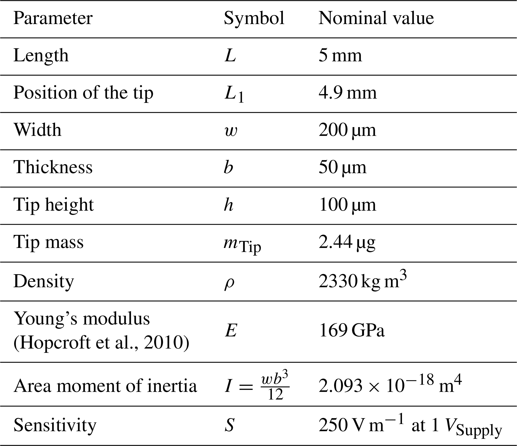
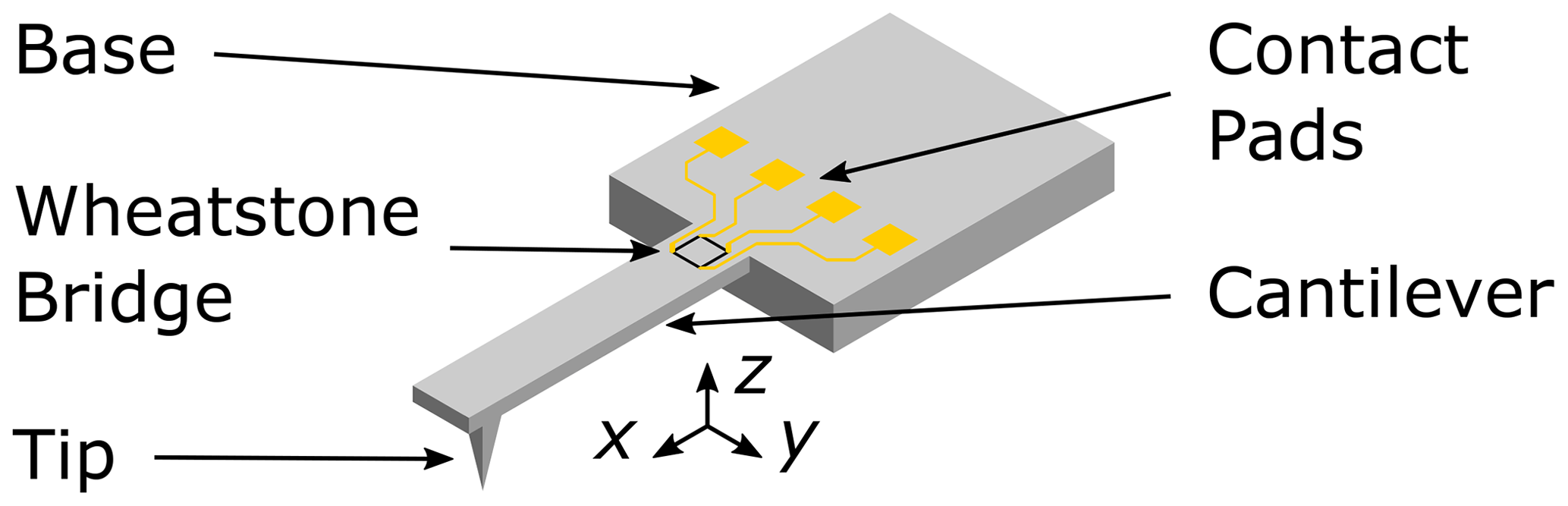
As shown in Fig. 1, the type of microprobe used in this study is a silicon cantilever with a tip at its free end and a Wheatstone bridge near the anchor point. These microprobes are commercially available (CAN50-2-5, CiS Forschungsinstitut für Mikrosensorik GmbH, 2019). Their nominal geometry is listed in Table 1.

The Wheatstone bridge of the sensors consists of four piezoresistors that are implanted into the cantilever close to its clamped end. At the output, the bridge supplies a voltage which is proportional to the strain (in the x direction) the resistor experiences. At low frequencies, i.e., when scanning the tip of the sensor across the surface of a sample, time-dependent behavior can be neglected, and the strain in the cantilever is proportional to the deflection of the tip. It is therefore possible to measure the height profile of a surface by recording the output voltage of the sensor.

Table 1 Geometrical and mechanical parameters of the microprobe (CiS Forschungsinstitut für Mikrosensorik GmbH, 2018).

Figure 1 Schematic of the microprobe.

2.1 Dynamic behavior of the microprobe

To additionally acquire information about the mechanical properties of the surface, the effects of the dynamic interaction between tip and surface are analyzed. As shown in Fig. 2, it is considered that the tip of the probe is in contact with the surface of the sample while the base is actuated harmonically. An actuation in the z direction shall create flexural vibrations in the cantilever, to which the surface of the sample will react via both its elasticity and viscosity. Elastic behavior is modeled by the normal and lateral contact stiffnesses k^* and $k_{\mathrm{Lat}}^{*}$; viscous behavior is modeled by the normal and lateral contact damping parameters γ^* and ${\mathit{\gamma }}_{\mathrm{Lat}}^{*}$. According to the Hertz theory, the normal contact stiffness is given by

$$\begin{array}{}\text{(1)}& k^{*}={\displaystyle \frac{\mathrm{3}}{\mathrm{2}}}{E}_{\mathrm{tot}}\times \sqrt{R}\times \sqrt{D},\end{array}$$

where R is the radius of the tip if the probe D is the deformation of the sample, and E_tot is the reduced elastic modulus given by

$$\begin{array}{}\text{(2)}& {\displaystyle \frac{\mathrm{1}}{E_{\mathrm{tot}}}}={\displaystyle \frac{\mathrm{3}}{\mathrm{4}}}\left({\displaystyle \frac{\mathrm{1}-{\mathit{\nu }}^{\mathrm{2}}}{E}}+{\displaystyle \frac{\mathrm{1}-{\mathit{\nu }}_{\mathrm{t}}^{\mathrm{2}}}{E_{\mathrm{t}}}}\right).\end{array}$$

Here, ν and E are Poisson's ratio and Young's modulus of the surface of the sample, respectively, while ν_t and E_t are Poisson's ratio and Young's modulus of the tip of the probe, respectively (Cappella, 2016).

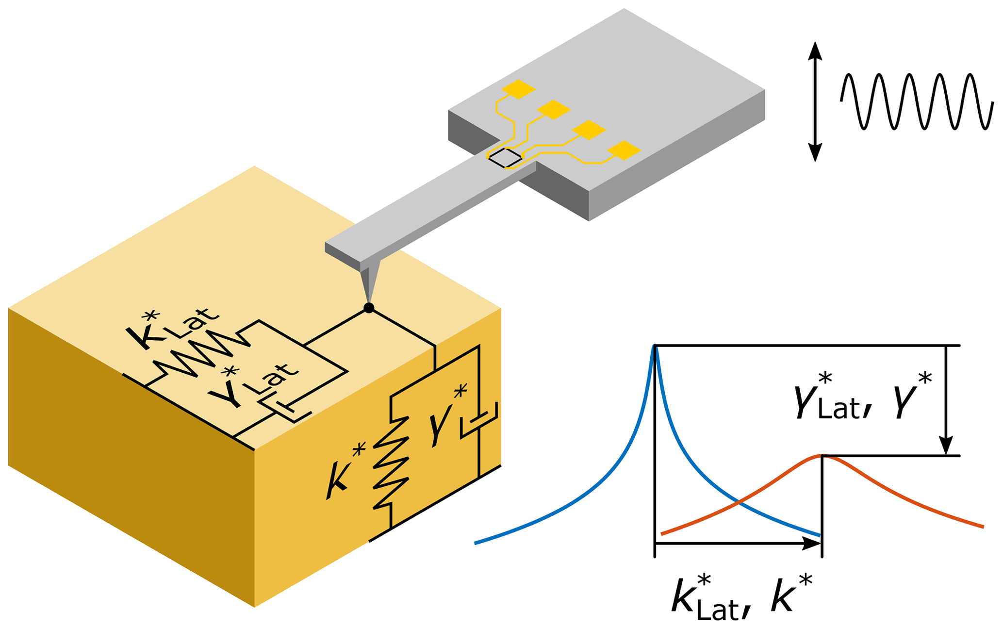
Figure 2 Schematic of the tip–surface interaction during out-of-plane bending vibration of the cantilever. The interaction is split into normal forces and lateral forces (with respect to the surface of the sample). Elastic behavior of the sample is modeled by the contact stiffnesses k^* and $k_{\mathrm{Lat}}^{*}$, respectively, while the viscous behavior is modeled by the contact damping parameters γ^* and ${\mathit{\gamma }}_{\mathrm{Lat}}^{*}$, respectively. Increasing the stiffness will lead to an increase in resonance frequency, while increasing the damping will reduce the resonance quality factor. Representation inspired by Kocun and Ohler (2013).

In her publication (Rabe, 2006), Rabe derived a model, which predicts the dynamic behavior of such a surface-coupled beam when excited into out-of-plane bending-mode vibrations. According to the procedure described there, the theoretical behavior of the setup used in this study is analyzed. Generally, a cantilever beam has to conform to the equation of motion

$$\begin{array}{}\text{(3)}& {\displaystyle \frac{EI}{\mathit{\rho }wb}}{\displaystyle \frac{{\partial }^{\mathrm{4}}z}{\partial x^{\mathrm{4}}}}+{\displaystyle \frac{{\partial }^{\mathrm{2}}z}{\partial t^{\mathrm{2}}}}+{\mathit{\eta }}_{\mathrm{Air}}{\displaystyle \frac{\partial z}{\partial t}}=\mathrm{0},\end{array}$$

where E is Young's modulus of the cantilever, I is the area moment of inertia, ρ is the mass density, w is the width, b is the thickness, z is the deflection of the neutral fiber of the cantilever at the position x and the time t, and η_Air is a damping constant that describes energy dissipation by air. The equation of motion is solved by

$$\begin{array}{}\text{(4)}& z(x,t)=R\left\{Z\left(x\right)\times e^{i\mathit{\omega }t}\right\},\end{array}$$

where Z(x) is a complex-valued shape function that describes the dependence of the deflection on the position and ω is the angular frequency of the excitation. As the tip of the probe is located though close to, but not exactly at, the free end of the cantilever, two different shape functions Z₁ and Z₂ have to be considered in their respective regions according to

$$\begin{array}{}\text{(5)}& Z\left(x\right)=\left\{\begin{array}{ll}{Z}_{\mathrm{1}}\left(x\right)& \mathrm{0}\le x\le L_{\mathrm{1}}\\ Z_{\mathrm{2}}(L-x)& L_{\mathrm{1}}<x\le L\end{array}\right..\end{array}$$

The function Z₁(x) begins at the anchor point at x=0 and ends at the position of the tip at x=L₁, while $Z_{\mathrm{2}}(L-x)=Z_{\mathrm{2}}\left(x^{\prime }\right)$ begins at the free end of the cantilever and ends at the position of the tip at x=L₁. For simplicity x^′ and L₂ are defined as follows:

$$\begin{array}{}\text{(6)}& x^{\prime }=L-x\mathrm{and}{L}_{\mathrm{2}}=L-L_{\mathrm{1}}.\end{array}$$

Using these conventions, the shape functions Z₁(x) and Z₂(x^′) are given by

$$\begin{array}{}\text{(7)}& {\displaystyle }& {\displaystyle }{Z}_{\mathrm{1}}\left(x\right)=c_{\mathrm{1}}\cosh \mathit{\alpha }x+c_{\mathrm{2}}\sinh \mathit{\alpha }x+c_{\mathrm{3}}\cos \mathit{\alpha }x+c_{\mathrm{4}}\sin \mathit{\alpha }x,\text{(8)}& {\displaystyle }& {\displaystyle }{Z}_{\mathrm{2}}\left(x^{\prime }\right)=c_{\mathrm{5}}\cosh \mathit{\alpha }{x}^{\prime }+c_{\mathrm{6}}\sinh \mathit{\alpha }{x}^{\prime }+c_{\mathrm{7}}\cos \mathit{\alpha }{x}^{\prime }+c_{\mathrm{8}}\sin \mathit{\alpha }{x}^{\prime },\end{array}$$

where c₁–c₈ are constants and α is the wave number of the flexural waves given by

$$\begin{array}{}\text{(9)}& {\mathit{\alpha }}^{\mathrm{4}}={\displaystyle \frac{\mathit{\rho }wb}{EI}}\left({\mathit{\omega }}^{\mathrm{2}}-i{\mathit{\eta }}_{\mathrm{Air}}\mathit{\omega }\right).\end{array}$$

To solve these equations, a set of eight boundary conditions is required. As the cantilever is clamped to the base of the probe at the anchor point, the excitation that is applied to the base acts on the clamped end of the beam as well. Therefore, the position of the beam is given by the amplitude z₀ of the excitation. Additionally, the clamping causes the slope of the beam to be zero:

$$\begin{array}{}\text{(10)}& Z_{\mathrm{1}}\left(\mathrm{0}\right)=z_{\mathrm{0}}\mathrm{and}{\displaystyle \frac{\partial Z_{\mathrm{1}}}{\partial x}}\left(\mathrm{0}\right)=\mathrm{0}.\end{array}$$

At the position of the tip, the partial solutions Z₁(x) and Z₂(x^′) have to merge continuously:

$$\begin{array}{}\text{(11)}& Z_{\mathrm{1}}\left(L_{\mathrm{1}}\right)=Z_{\mathrm{2}}\left(L_{\mathrm{2}}\right)\mathrm{and}{\displaystyle \frac{\partial Z_{\mathrm{1}}}{\partial x}}\left(L_{\mathrm{1}}\right)=-{\displaystyle \frac{\partial Z_{\mathrm{2}}}{\partial x^{\prime }}}\left(L_{\mathrm{2}}\right).\end{array}$$

The negative sign in the right-hand part of Eq. (11) appears because x^′ is defined in the negative direction of x. Furthermore, the interaction between tip and sample has to be considered at this position, i.e., at x=L₁. Equation (12) couples the bending moment of the cantilever and the tip with the lateral reactionary forces at the surface of the sample. Here, h is the height of the tip, m_Tip is its mass, and r is the distance between the neutral fiber of the cantilever and the center of mass of the tip. Equation (13) describes the equilibrium of shear forces at the tip.

$$\begin{array}{}\text{(12)}& {\displaystyle }\begin{array}{rl}{\displaystyle \frac{{\partial }^{\mathrm{2}}{Z}_{\mathrm{1}}}{\partial x^{\mathrm{2}}}}& \left(L_{\mathrm{1}}\right)-{\displaystyle \frac{{\partial }^{\mathrm{2}}{Z}_{\mathrm{2}}}{\partial {x^{\prime }}^{\mathrm{2}}}}\left(L_{\mathrm{2}}\right)=-{\displaystyle \frac{h^{\mathrm{2}}}{EI}}\\ & \times \left(k_{\mathrm{Lat}}^{*}+i\mathit{\omega }{\mathit{\gamma }}_{\mathrm{Lat}}^{*}-m_{\mathrm{Tip}}{\mathit{\omega }}^{\mathrm{2}}{\displaystyle \frac{L_{\mathrm{1}}}{L}}{\displaystyle \frac{r^{\mathrm{2}}}{h^{\mathrm{2}}}}\right)\times {\displaystyle \frac{\partial Z_{\mathrm{1}}}{\partial x}}\left(L_{\mathrm{1}}\right)\end{array}\text{(13)}& {\displaystyle }\begin{array}{rl}{\displaystyle \frac{{\partial }^{\mathrm{3}}{Z}_{\mathrm{1}}}{\partial x^{\mathrm{3}}}}& \left(L_{\mathrm{1}}\right)+{\displaystyle \frac{{\partial }^{\mathrm{3}}{Z}_{\mathrm{2}}}{\partial {x^{\prime }}^{\mathrm{3}}}}\left(L_{\mathrm{2}}\right)={\displaystyle \frac{\mathrm{1}}{EI}}\\ & \times \left(k^{*}+i\mathit{\omega }{\mathit{\gamma }}^{*}-m_{\mathrm{Tip}}{\mathit{\omega }}^{\mathrm{2}}{\displaystyle \frac{L_{\mathrm{1}}}{L}}\right)\times Z_{\mathrm{1}}\left(L_{\mathrm{1}}\right)\end{array}\text{(14)}& {\displaystyle }r={\displaystyle \frac{b}{\mathrm{2}}}+{\displaystyle \frac{h}{\mathrm{3}}}\end{array}$$

Equations (12) and (13) can be extended to include the effect of a tilt of the cantilever with respect to the surface of the sample. In this study, however, this effect is neglected, as during measurements the tilt only amounts to approximately 1^∘. At the free end of the beam both the bending moment and the shear force must be zero. The boundary conditions here are consequently

$$\begin{array}{}\text{(15)}& {\displaystyle \frac{{\partial }^{\mathrm{2}}{Z}_{\mathrm{2}}}{\partial {x^{\prime }}^{\mathrm{2}}}}\left(\mathrm{0}\right)=\mathrm{0}\mathrm{and}{\displaystyle \frac{{\partial }^{\mathrm{3}}{Z}_{\mathrm{2}}}{\partial {x^{\prime }}^{\mathrm{3}}}}\left(\mathrm{0}\right)=\mathrm{0}.\end{array}$$

Finally, a computer algebra system is used to determine the constants in the shape functions given in Eqs. (7) and (8) (Rabe, 2006).

2.2 Replicating the output signal of the microprobe

As mentioned in Sect. 2, the output voltage of the sensor is proportional to the strain that the piezoresistors experience. For practical purposes, however, the sensitivity of the sensor is not given in relation to strain, but in relation to the static deflection of the tip. The output voltage of the sensor follows as

$$\begin{array}{}\text{(16)}& U_{\mathrm{Out}}=U_{\mathrm{Supply}}\times S\times \mathit{\delta },\end{array}$$

where U_Supply is the supply voltage of the Wheatstone bridge and δ is the deflection of the cantilever at the position of the tip. To analyze dynamic behavior, it is necessary to calculate the sensitivity of the sensor in relation to the time-dependent strain:

$$\begin{array}{}\text{(17)}& U_{\mathrm{Out}}\left(t\right)=U_{\mathrm{Supply}}\times S_{\mathit{ϵ}}\times {\mathit{ϵ}}_x\left(t\right).\end{array}$$

Here, S_ϵ is the sensitivity in relation to strain and ϵ_x is the strain in the x direction the resistors, located at x_Bridge, experience. This equation also holds true during static operation. Therefore, combining the strain ϵ_x,Static caused by static deflection with Equ. (17) yields the strain sensitivity of the probe.

$$\begin{array}{}\text{(18)}& {\displaystyle }& {\displaystyle }{U}_{\mathrm{Out}}=U_{\mathrm{Supply}}\times S\times \mathit{\delta }=U_{\mathrm{Supply}}\times S_{\mathit{ϵ}}\times {\mathit{ϵ}}_{x,\mathrm{Static}}\text{(19)}& {\displaystyle }& {\displaystyle }{S}_{\mathit{ϵ}}={\displaystyle \frac{S\times \mathit{\delta }}{{\mathit{ϵ}}_{x,\mathrm{Static}}}}\text{(20)}& {\displaystyle }& {\displaystyle }{\mathit{ϵ}}_{x,\mathrm{Static}}=-{\displaystyle \frac{\mathrm{3}b\mathit{\delta }}{\mathrm{2}{L}_{\mathrm{1}}^{\mathrm{3}}}}\times \left(L_{\mathrm{1}}-x_{\mathrm{Bridge}}\right)\text{(21)}& {\displaystyle }& {\displaystyle }{S}_{\mathit{ϵ}}=-{\displaystyle \frac{\mathrm{2}{L}_{\mathrm{1}}^{\mathrm{3}}S}{\mathrm{3}b\left(L_{\mathrm{1}}-x_{\mathrm{Bridge}}\right)}}\end{array}$$

Now, the time-dependent strain is calculated to replicate the behavior of the probe:

$$\begin{array}{}\text{(22)}& {\mathit{ϵ}}_x\left(t\right)=-{\displaystyle \frac{b}{\mathrm{2}}}\times {\displaystyle \frac{{\partial }^{\mathrm{2}}z}{\partial x^{\mathrm{2}}}}\left(x_{\mathrm{Bridge}},t\right).\end{array}$$

This formula also includes the actuation amplitude, as it is contained in one of the boundary conditions presented in Sect. 2.1. The actuation amplitude is given by

$$\begin{array}{}\text{(23)}& z_{\mathrm{0}}=S_{\mathrm{Actuator}}\times U_{\mathrm{Actuator}},\end{array}$$

with the actuation sensitivity S_Actuator and the actuation voltage U_Actuator. Here, the actuation sensitivity is the relation between the applied voltage and the resulting displacement. Finally, a preamplifier with the gain G is considered, resulting in the measured voltage U_Measured(t) given by

$$\begin{array}{}\text{(24)}& U_{\mathrm{Measured}}\left(t\right)=G\times U_{\mathrm{Supply}}\times S_{\mathit{ϵ}}\times {\mathit{ϵ}}_x\left(t\right)\end{array}$$

(Gross et al., 2014).

Although the formula to replicate measured behavior is finished, it cannot be used, yet. Some parameters, like η_Air and S_Actuator, are still unknown, while geometrical parameters might need to be adjusted as idealizations of the model can lead to discrepancies between measured and calculated values (Hurley, 2009). Furthermore, using four independent parameters to describe the interaction between tip and surface is not practical. For every frequency that is tested, only two values can be extracted: the vibration amplitude and the vibration phase. Therefore, only two independent values, which describe the interaction, can be obtained. For this reason, the lateral elements $k_{\mathrm{Lat}}^{*}$ and ${\mathit{\gamma }}_{\mathrm{Lat}}^{*}$ are coupled to their normal counterparts k^* and γ^*:

$$\begin{array}{}\text{(25)}& {\displaystyle \frac{k_{\mathrm{Lat}}^{*}}{k^{*}}}={\displaystyle \frac{{\mathit{\gamma }}_{\mathrm{Lat}}^{*}}{{\mathit{\gamma }}^{*}}}=\mathrm{const}.\end{array}$$

However, the constant of proportionality is unknown as well. Procedures to obtain numerical values of these unknown parameters are discussed in Sect. 4.

3 Measurement setup

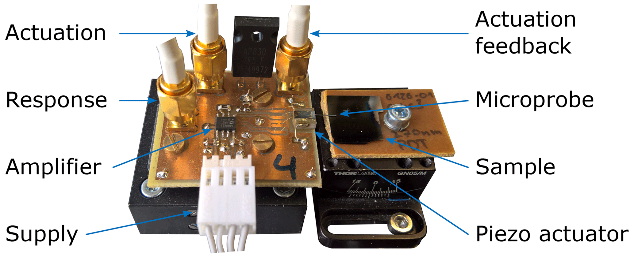
Before measurements can be conducted, the probes have to be connected both mechanically and electrically to a measurement setup. As shown in Fig. 3, the microprobes are mounted on so-called carrier PCBs that incorporate a piezoactuator (5 mm × 5 mm × 2 mm, PL 055.30 PICMA^® Chip Actuator, PI Ceramic) to excite the probe and a preamplifier (AD8421, Analog Devices Inc.) to buffer and boost the output signal of the sensor. The actuation and response signals are supplied and measured, respectively, by custom measurement electronics (Fahrbach et al., 2018) that are connected to the carrier PCB via SMA ports. Additionally, a pin header is used to supply power to the amplifier and the sensor.

Figure 3 Photograph of a microprobe carrier PCB next to a sample under test.

The carrier PCB is mounted on a positioning system, shown in Fig. 4, which allows for positioning in the xy plane using manual stages and positioning in the yz plane using piezo stages (PI P-518.ZCD and PI P-621.1CD, Physik Instrumente (PI) GmbH & Co.KG). The sample under test is mounted on a separate manual xyz stage next to the microprobe.

Figure 4 Photograph of the homemade positioning and scanning table with a microprobe carrier PCB mounted on top. The tip of the probe is in contact with the surface of a sample, which is mounted on a manual xyz stage.

In the beginning of a measurement, the probe is positioned close to the surface of the sample using the manual stages. Afterwards, the probe is moved in the direction of the sample using the piezo z stage, until contact between tip and surface is established and the cantilever begins to bend. This movement is continued until the force the cantilever exerts on the sample, which is equal to the product of stiffness and deflection of the beam, reaches a set value. Hereafter, the piezoactuator beneath the probe is used to excite the cantilever into out-of-plane bending-mode vibrations.

4 Calibration

The first variable of the vibration model to be calibrated is the sensitivity of the sensor. The sensitivity can be measured by deflecting the cantilever in a quasi-static manner against a silicon wafer considered an indeformable sample. While displacing the cantilever, the position and output voltage of the probe are recorded. A typical sensitivity-calibration curve is shown in Fig. 5.

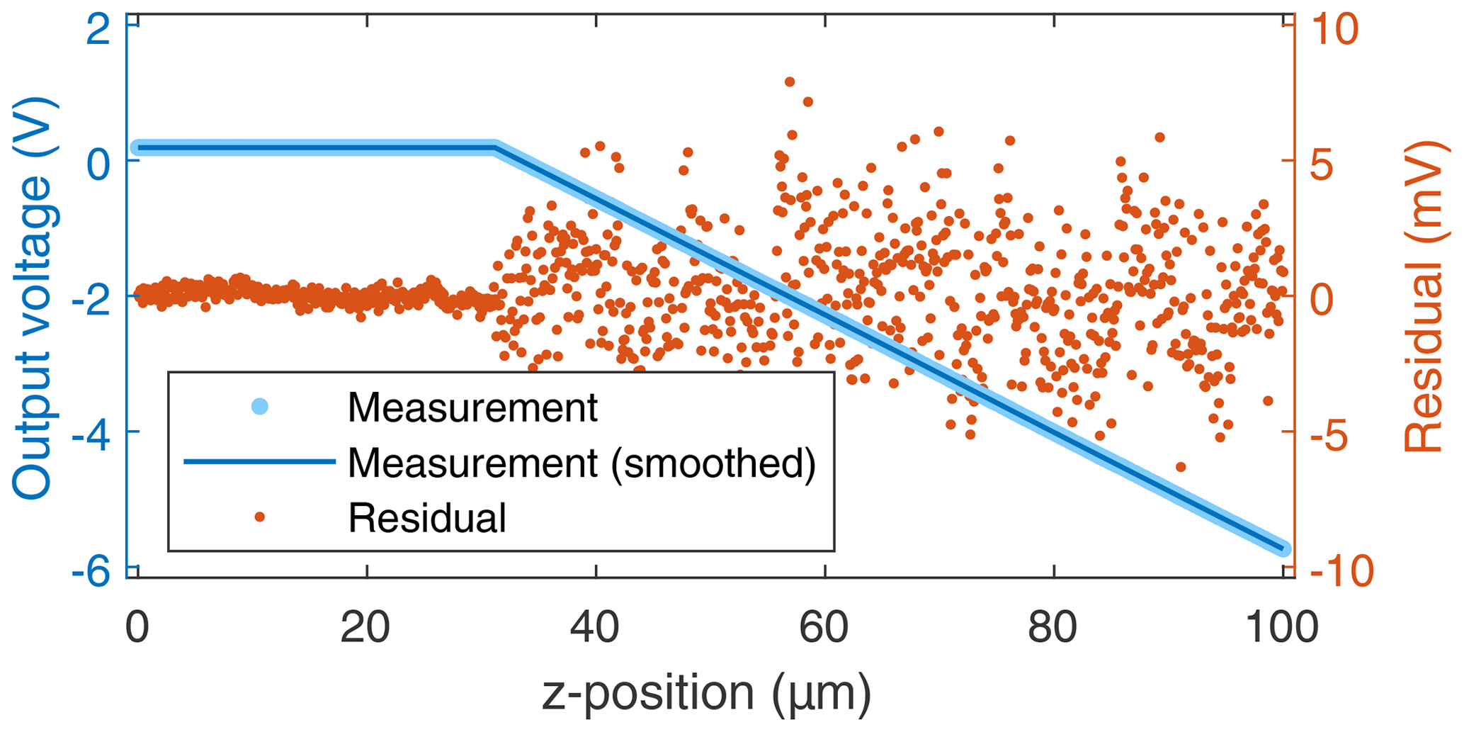
Figure 5 Quasi-static voltage-displacement curve. Measured values (light blue dots) and smoothed curve (dark blue line). To illustrate the agreement between measurement and extracted information, residuals are shown as red dots on a magnified scale given on the right ordinate.

In the beginning of the measurement the tip of the probe has yet to touch the surface of the sample. Therefore, the output voltage remains at a constant value. Once contact has been established, the voltage decreases with increasing displacement. When using a supply of U_Supply=3.4 V and an analog gain of G=100, the output of the carrier PCB should drop by ca. 85 mV for every micrometer of deflection, according to the datasheet. As depicted in Fig. 6, the measured sensitivity deviates from the nominal value by up to 2.3 mV µm⁻¹ and averages out at 86 mV µm⁻¹, which is well within production tolerance. However, a dependence of the sensitivity from the deflection of the beam is observed.

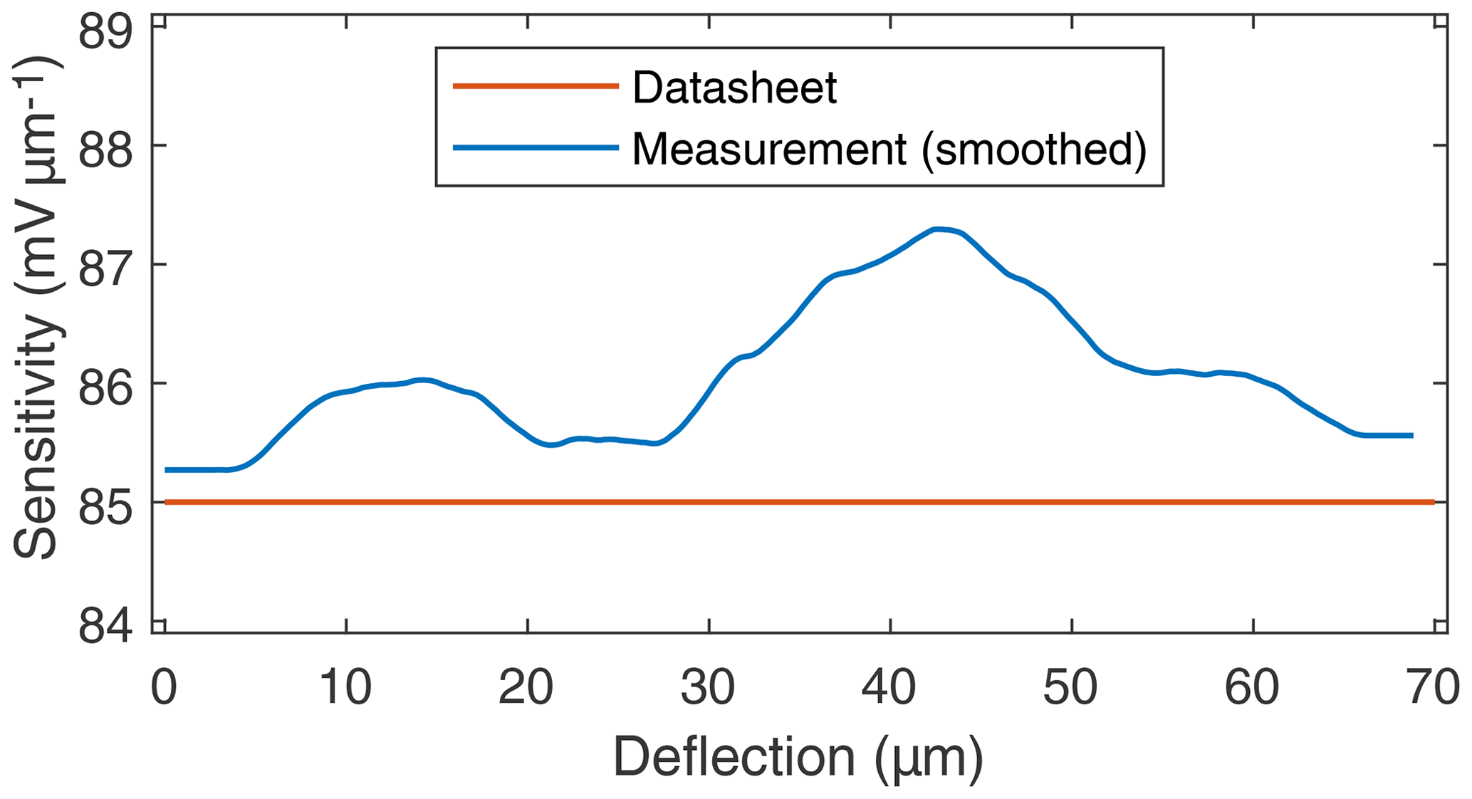
Figure 6 Sensitivity of the microprobe. Value given in datasheet (red) and measured values (blue).

When analyzing a deformable sample, a displacement curve similar to Fig. 5 is measured. Here, the deformation of the sample is given by Cappella (2016):

$$\begin{array}{}\text{(26)}& D=z-z_{\mathrm{contact}}-\mathit{\delta },\end{array}$$

where z is the position of the probe, z_contact is the point where contact between tip and surface is first established, and δ is the deflection of the cantilever. Using the reference measurement, the measured voltage is related to the deflection of the beam:

$$\begin{array}{}\text{(27)}& \mathit{\delta }={\mathit{\delta }}_{\mathrm{reference}}\left(U_{\mathrm{Measured}}\right).\end{array}$$

Thus, the deformation of the sample under test is calculated as

$$\begin{array}{}\text{(28)}& D=z-z_{\mathrm{contact}}-{\mathit{\delta }}_{\mathrm{reference}}\left(U_{\mathrm{Measured}}\right).\end{array}$$

For this procedure to yield reasonable data, the non-constant sensitivity, i.e., the deviation from linearity shown in Fig. 6, has to be determined for each sensor.

In the next step, measurements of the out-of-plane vibration modes are conducted. Figure 7 shows a Bode plot of the first vibration mode. From these curves, the resonance frequency, Q factor, and amplitude can be extracted to gain information about the geometry of the cantilever, air damping, and the sensitivity of the actuator.

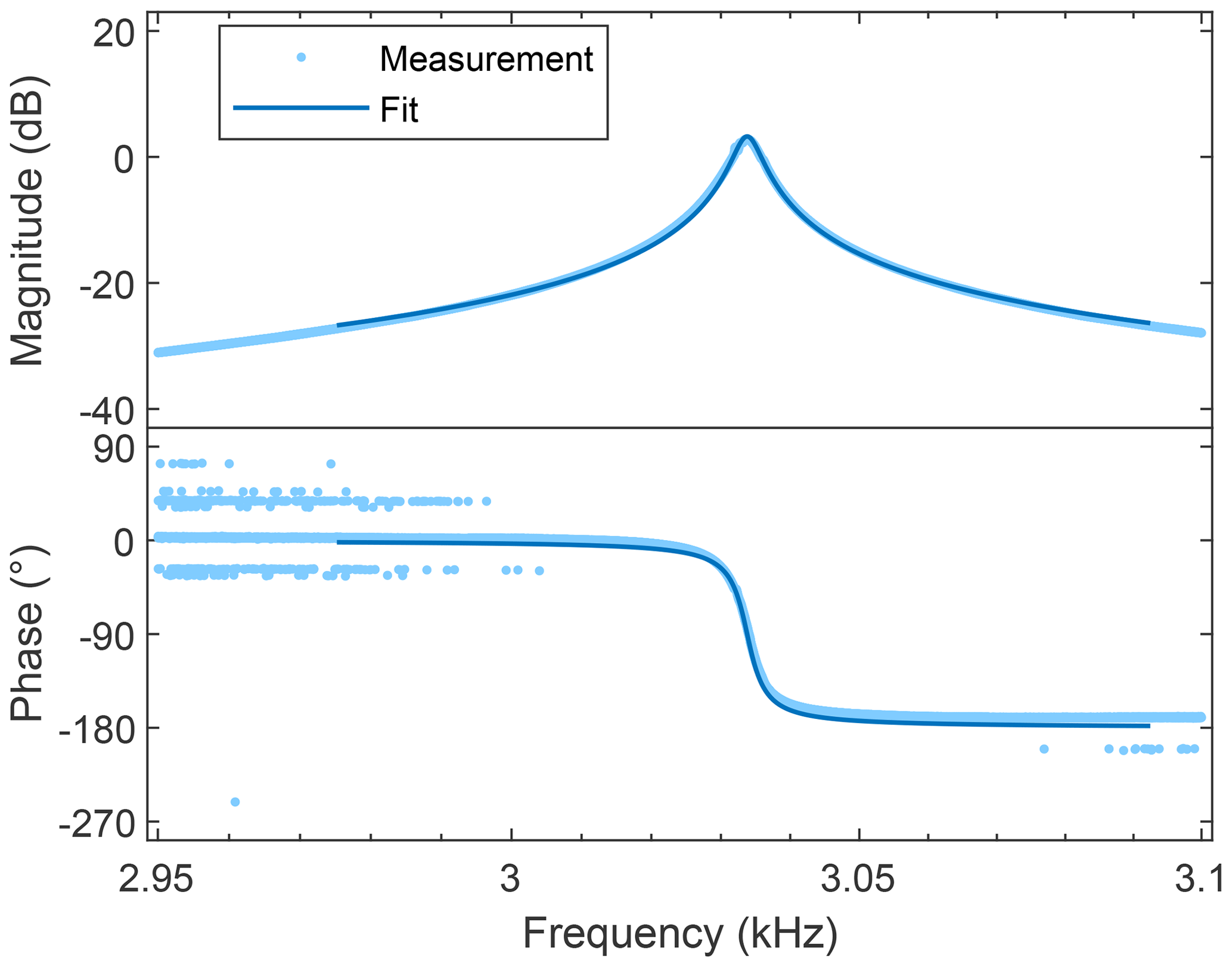
Figure 7 Bode plot of the first out-of-plane bending-mode resonance peak. Measured values (light blue dots) and fit of the model (dark blue line).

At first, the measured resonance frequency values are used to check and, if necessary, adjust the geometry of the cantilever (in the model). As the length and width of the beam can be controlled precisely during production, errors between nominal and real values are assumed to be negligible. Most likely, the deviations between measured resonance frequencies and calculated values are the result of the thickness deviating from its nominal value.

As shown in Fig. 8, the resonance frequencies calculated using the nominal geometry are consistently lower than measured values. By increasing the assumed thickness of the cantilever to 56.6 µm, the deviations between calculations and measurements decrease to less than 1 %. The remaining errors can be explained by geometric deviations that are not yet accounted for, like the shape of the tip, and by the fact that idealizations of the model only describe reality by approximation. To consider the remaining deviations, a compensating curve to rescale the frequency axis of the vibration model is used. Otherwise it would not be possible to precisely fit the model to all measured resonance modes.

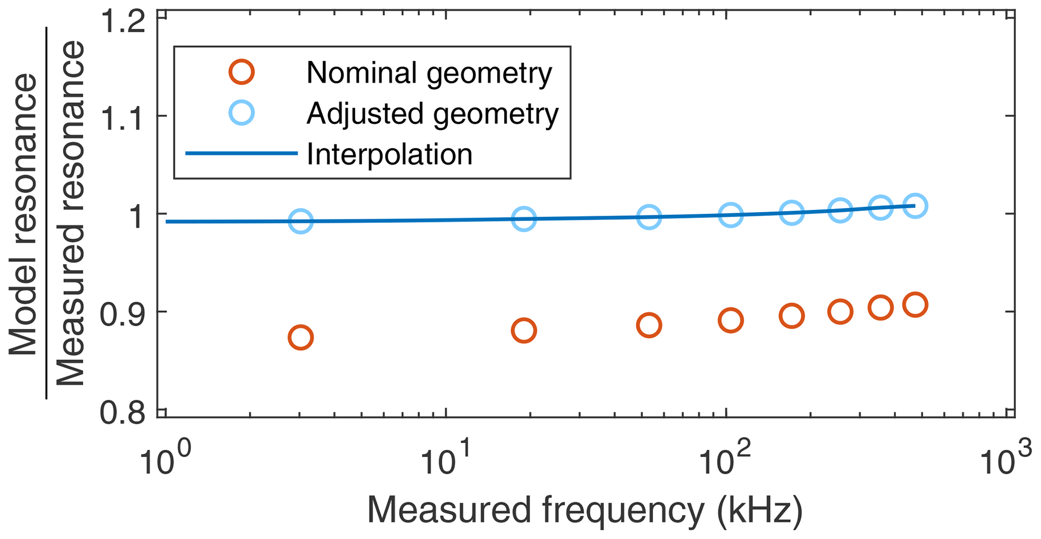
Figure 8 Resonance frequencies of the model in relation to the measured values. Nominal values are calculated using the geometry of the sensor given in the datasheet, and adjusted values are calculated after adjusting the geometry to minimize the error. Additionally, a compensating curve is shown which is used for subsequent calculations.

After ensuring that the calculated resonance frequencies match the measured values, the model is fitted to the measured resonance curves, as shown in Fig. 7. Thus, one value each of the air-damping constant and the sensitivity of the actuator is extracted from every resonance peak, respectively. The values of the air-damping constant are shown in Fig. 9. They are used to generate a compensating curve to calculate damping values for arbitrary frequencies. As described by Rabe (2006), the damping increases with the frequency. Since the value of this constant is not known in advance, however, it is not possible to draw any conclusions from the data obtained.

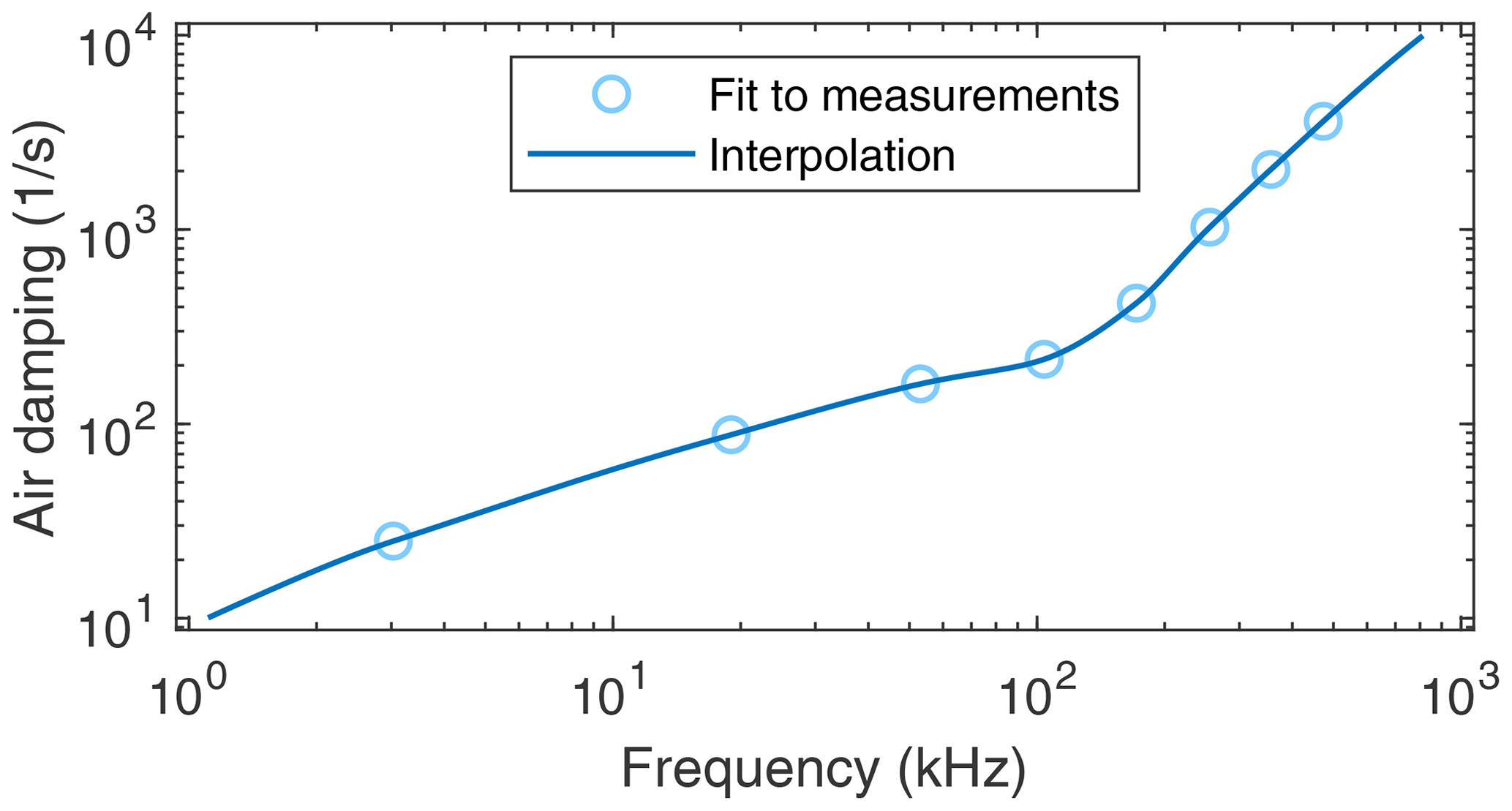
Figure 9 Frequency response of air damping, as determined by fitting the vibration model to resonance peaks of eight out-of-plane bending-vibration modes.

Now, resonance peaks of the microprobe in contact with a sample, as shown in Fig. 10, are measured. The polymer Poly(n-butyl methacrylate), short PnBMA, is chosen as the sample material, as it shows no frequency dependence in the frequency range that is to be analyzed. All contact resonance modes are measured on the same sample under the same conditions. As with the previous resonance curves, the vibration model is fitted to these peaks. For every resonance peak, respectively, this results in one value each of the contact stiffness, the contact damping, and the sensitivity of the actuator. As all resonance modes are analyzed under the same conditions, the fits should yield the same contact stiffnesses (Hurley, 2009). If this is not the case, the position of the tip, which is used for the calculations, and the constant that couples the normal and lateral forces must be adjusted. As discussed in Sect. 2.2, the geometry used for calculations does not have to match the physical dimensions of the probe.

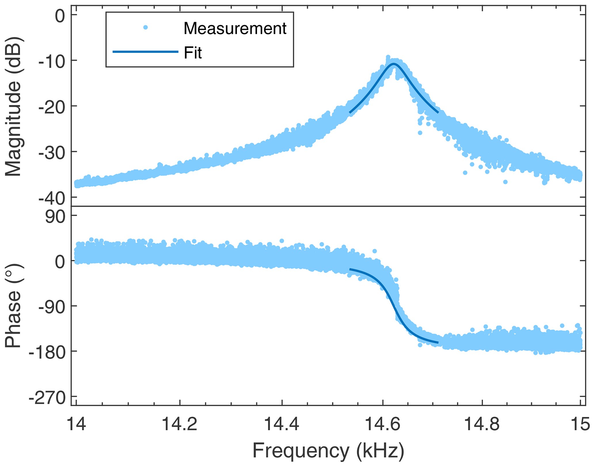
Figure 10 Bode plot of the first out-of-plane bending-mode contact resonance peak, measured on a thin film of PnBMA polymer (light blue dots) and a fit of the model (dark blue line).

In the next step, the frequency response of the sensitivity of the actuator, i.e., the relation between the applied voltage and the resulting displacement, is evaluated. Several values of the sensitivity are computed when fitting the measured peaks of the resonance modes. The resulting data are shown in Fig. 11. To ensure the validity of the calculated values, all resonance peaks are measured multiple times. When the cantilever is vibrating in air, these curves are highly reproducible. Here, errors of the sensitivity below 3 % are observed (e.g., 2.38 %) when comparing two measurements of the second out-of-plane resonance mode taken at a time interval of 230 d. This error is assigned to ambient-temperature changes between the measurements, thereby shifting the sensitivity of the probe slightly. It can be removed by calibrating the sensitivity of the probe at different temperatures. When in contact with a sample, the standard deviation of the mean of the sensitivity of the piezoactuator increases to 3 %, 6 % and 3 % for the first, second, and third contact resonance modes, respectively. As shown in Fig. 11, the computed values are lower than the nominal value given in the datasheet. This might be due to carrier–PCB-induced damping of the vibration. It is unknown, however, whether damping alone can explain a decline in sensitivity by 2 orders of magnitude.

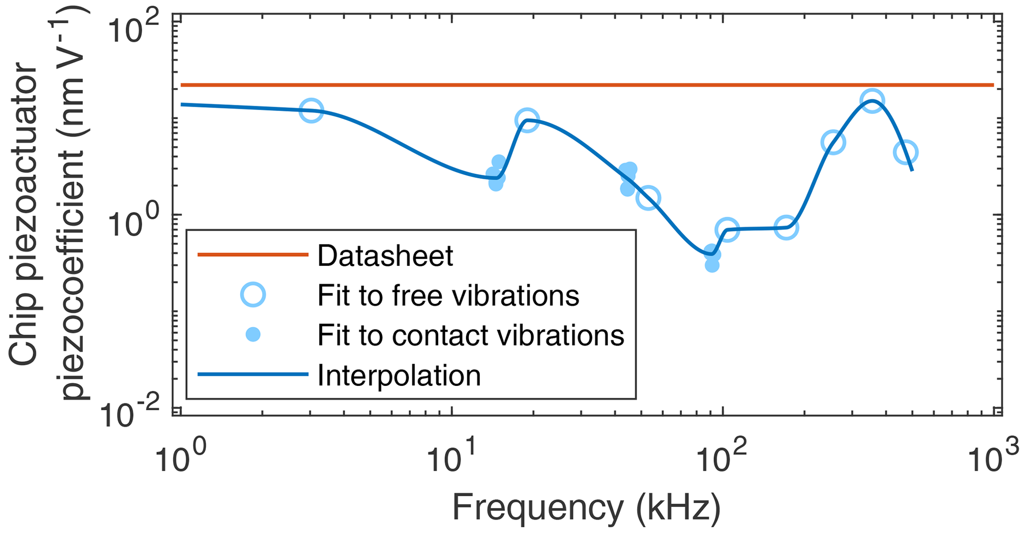
Figure 11 Frequency response of the sensitivity of the piezoactuator used in this work: sensitivity given in the datasheet (red line); values obtained by fitting the vibration model to measured resonance peaks of the sensor without contact (open blue circles) and with contact (filled blue circles) and interpolation through these values (blue line). The data points with contact represent 14, 10, and 10 measurements for the first, second, and third modes with standard deviations of the mean values of 3 % to 6 %.

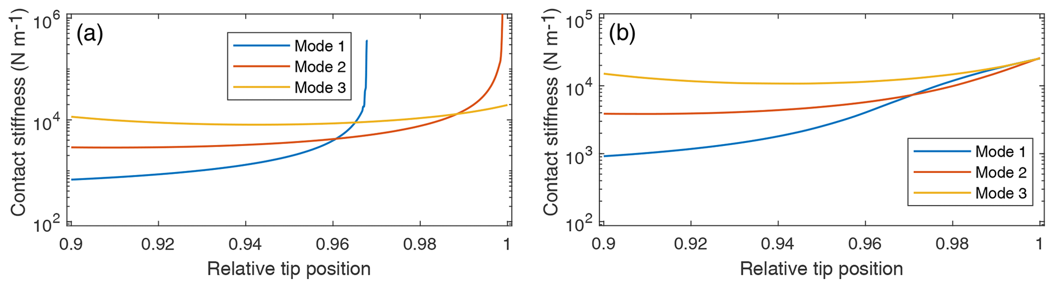
Figure 12 Calculated contact stiffness of the measured lowest three resonance peaks in dependence on the position of the tip for finding its most consistent value with (a) the length of the cantilever set to the specified value of L=5 mm (Table 1), whereby lateral forces are neglected. Here, the optimum tip position is $L_{\mathrm{1}}/L=\mathrm{0.964}$. (b) If the lengths of the cantilever and lateral elements are set to L=5.555 mm and $k_{\mathrm{Lat}}^{*}/k^{*}={\mathit{\gamma }}_{\mathrm{Lat}}^{*}/{\mathit{\gamma }}^{*}=\mathrm{0.444}$, respectively, intersecting curves for all three modes are found at an optimum tip position of $L_{\mathrm{1}}/L=\mathrm{0.999}$.

On the other hand, if the sensitivity is not adjusted according to the fits, measured resonance amplitudes (e.g., in Fig. 10) cannot be reproduced by the model. Contact damping parameters calculated under these conditions are not further used. When applying the calibration and taking the error of the calibrated values into account, the error of the contact damping parameter is approximately ±15 %. The effect of calibration on the contact stiffness is negligible; i.e., contact stiffness only deviates by less than 1 % from values calculated without calibrating the sensitivity. To be able to reproduce measured amplitude and phase characteristics (cf., Fig. 10), the calibrated values of piezoactuator sensitivity in Fig. 11 are used for the subsequent calculations. Interpolation of the data points is used to provide values of the sensitivity at arbitrary frequencies in the range of 1 to 500 kHz.

The subsequent step in the calibration is to calculate a position of the tip, which results in the best agreement of the contact stiffnesses of all contact resonance peaks used for the calibration. This is done by choosing a selection of different positions, performing all previous steps of calibration for them, and, as shown in Fig. 12a, comparing the calculated contact stiffnesses. The position with the lowest deviation between the modes is assumed to be the most consistent.

There are several shortcomings resulting from this procedure, nevertheless. Firstly, not all modes yield usable data for the entire range of selected tip positions. In the case of the first resonance mode, for example, using values above 0.97, the calculated stiffness increases to infinity; i.e., the model cannot reproduce the measured frequency. Furthermore, there is no unique point of intersection of all three curves.

To achieve better agreement between the modes, the length of the cantilever is taken as a further adjustable parameter. As with the calibration of the position of the tip, a range of values is considered for the length of the cantilever. Afterwards, all previous calibrations are repeated and the resulting contact stiffnesses are evaluated. The length that results in the best agreement of the three modes is chosen as the optimal value. As shown in Fig. 13a, lateral forces have a decisive effect; i.e., when they are neglected, no intersection is detected between the modes. To achieve this, the lateral forces acting on the tip are included.

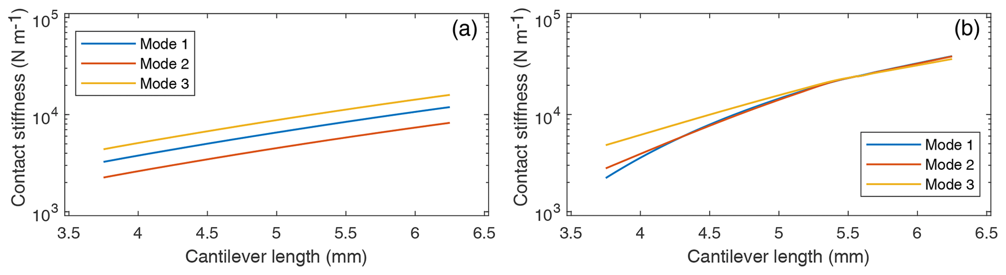
Figure 13 Calculated contact stiffness of the measured lowest three resonance peaks. Varying the assumed length of the cantilever improves the consistency of the model calculations. (a) Lateral forces are neglected in this evaluation. No clear optimum cantilever length is found in this case. (b) Lateral elements are set to $k_{\mathrm{Lat}}^{*}/k^{*}={\mathit{\gamma }}_{\mathrm{Lat}}^{*}/{\mathit{\gamma }}^{*}=\mathrm{0.444}$. Here, an optimum cantilever length is visible at L=5.555 mm.

The procedure of finding the optimum value of the lateral forces is similar to the previous two steps. A selection of values for the coupling constant between the normal and lateral forces is chosen, and the length of the cantilever is optimized for each of them. The resulting contact stiffnesses are compared, and the coupling constant, which results in the lowest deviation, is chosen as the best value. By adjusting the lateral elements to $k_{\mathrm{Lat}}^{*}=\mathrm{0.444}\times k^{*}$ and ${\mathit{\gamma }}_{\mathrm{Lat}}^{*}=\mathrm{0.444}\times {\mathit{\gamma }}^{*}$, respectively, as shown in Fig. 14, the length of the cantilever to L=5.555 mm, as shown in Fig. 13b, and the position of the tip to L₁=5.551 mm, as shown in Fig. 12b, the deviations between the modes are reduced considerably. Obviously, the tip of the probe is located in close proximity of the free end of the cantilever. For the cantilever probes investigated in this study, it is therefore not necessary to consider a cantilever model split into two parts, as described in Sect. 2.1. Instead, a greatly simplified model with the tip located at the free end can be employed.

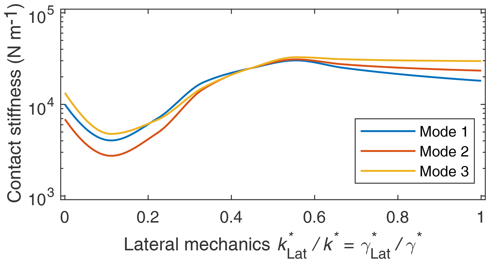
Figure 14 Calculated contact stiffness of the measured lowest three resonance peaks in dependence on lateral surface interactions. Best model consistency can be expected at the intersection point of the three analyzed modes at $k_{\mathrm{Lat}}^{*}/k^{*}={\mathit{\gamma }}_{\mathrm{Lat}}^{*}/{\mathit{\gamma }}^{*}=\mathrm{0.444}$.

5 Results

After performing these calibrations, a number of measurements of a 610 nm thin film of Poly(n-butyl methacrylate), short PnBMA, are conducted. This polymer is supplied by Sigma Aldrich and has a typical molecular weight of 337 000. The film is spin coated from toluene on glass. During the measurements, the contact resonance frequencies of three out-of-plane vibration modes are analyzed at different contact forces. Afterwards, the deformation of the sample is calculated corresponding to Eq. (28). For each deformation, the resonance frequency is measured at 11 different positions on the sample with 1000 measured frequency values each. Then, the corresponding contact stiffnesses are determined using optimization algorithms to replicate the measured resonance frequencies and amplitudes with the model. According to Eq. (1), the calculated contact stiffnesses are fitted with a square root dependence on deformation. This shows good agreement between theory and calculated values, with the root mean squared error of the fits (807, 612, and 1197 N m⁻¹ for the first, second, and third modes, respectively) being lower than the mean standard deviations of the calculated stiffnesses (940, 1327, and 1560 N m⁻¹ for the first, second, and third modes, respectively).

Identical contact stiffness-deformation curves, which are expected according to Hurley (Hurley, 2009), are not found for the different vibration modes. In contrast, the contact stiffness is found to increase with increasing vibration mode, especially at larger deformations. A reason may be that the coupling of normal and lateral forces depends on the deformation. Remaining inconsistencies after calibration between the contact-stiffness/deformation plots of the modes (Fig. 15) might be removed by increasing the number of reference measurements and calibration steps, respectively.

Figure 15 Contact stiffness calculated from measurements on a PnBMA polymer film. By performing calibrations, good agreement between the modes of vibration is obtained.

6 Conclusions

In this study, a model to analyze contact resonance measurements was created systematically. The process to calibrate this model based on reference measurements was explained and discussed. A number of variables such as sensitivity of the sensor, air damping, sensitivity of the actuator, and geometrical values were considered. Finally, measurements on a polymer thin film were analyzed to verify the performance of the model.

Using this approach, good agreement between measurements and theory was achieved. The resulting data still show room for improvement, though. Firstly, the measurement setup will be made more reproducible to reduce errors. For this purpose, a new positioning system to reduce vibrations and positioning errors was procured. Additionally, a new electronic setup is in development for reducing measurement errors and increasing sensitivity. Afterwards, unexpected effects, like the frequency dependence of the sensitivity of the actuator, will be investigated further. A new set of reference measurements is in preparation, including measurements to be recorded at different deformations. Finally, the performance of our setup will be evaluated by comparing contact stiffnesses and damping parameters (and resulting Young's modulus and viscosity values) of thin polymer layers, with results determined using force-deflection curves and contact resonance spectrometry using our cantilevers in a Cypher AFM.