the Creative Commons Attribution 4.0 License.
the Creative Commons Attribution 4.0 License.
 | 02 Nov 2020
Intelligent fault detection of electrical assemblies using hierarchical convolutional networks for supporting automatic optical inspection systems
Alida Ilse Maria Schwebig
Rainer Tutsch
Electrical assemblies are the core of many electronic devices and therefore represent a crucial part of the overall product, which must be carefully checked before integration into its functional environment. For this reason, automatic optical inspection systems are required in electronic manufacturing to detect visible errors in products at an early stage. In particular, the automotive electronics production area is one of the sectors in which quality assurance has uppermost priority, as undetected defects can pose a danger to life. However, most optical inspection processes still have error slippage rates, which are responsible for delivering faulty electrical assemblies to customers. Therefore, this article shows how an application strategy of deep learning, based on neural networks, can be combined with an automatic optical inspection system to further increase the recognition accuracy of the process.
The additional use of artificial intelligence supported classification systems provides a way to find out the exact details about the manufacturing-related errors of electrical assemblies. However, due to the high number of different error categories, a single classification algorithm is usually not sufficient to provide reliable visual inspection results with high robustness against error slip. For this reason, a hierarchical model with multiple classifiers is proposed in this article. The principle is based on the hierarchical description of the quality status and fault types using several combined neural networks. In this context, the original classification task is distributed over different subnetworks. These subnetworks, which interact as an overall model, only verify certain error and quality features of the electrical assemblies, which means that higher recognition accuracy and robustness can be achieved compared to a single network.
- Article
(1708 KB) - Full-text XML
- BibTeX
- EndNote


During the production of electrical assemblies, manufacturing-related errors cannot be completely avoided without increasing cost and production time exponentially. As connection points between the components and the printed circuit board (PCB), solder joints are often most vulnerable to errors and defects. Hence, the quality of the solder joints directly influences the durability and reliability of the final product. For this reason, automatic optical inspection (AOI) systems are integrated as non-invasive testing processes in production lines to investigate failures on PCB, components, or solder joints during the manufacturing processes. As part of inspection, electrical assemblies are scanned and analyzed. At the same time, various image processing methods are used to detect quality defects in the inspection images of products (Berger, 2012). The continuous miniaturization effort and optimization of electronic devices leads to increased packaging density on PCB of electrical assemblies. With the associated increase in circuit complexity, the optical inspection is becoming progressively demanding (Niemann et al., 2017; Combet and Chang, 2009). This problem leads to new challenges in development of advanced automatic inspection systems.
Schwebig and Tutsch (2020) have already proposed the use of a deep learning concept to complement the optical inspection system in electronics production. In this paper, a novel defect detection system based on deep learning and focused on a practical industrial application was presented. With the help of an artificial intelligence (AI) supported classification system, an additional test procedure based on image detection for real-time visualization and analysis of electrical assemblies is to be implemented in a production line. The article shows an application strategy how a convolutional neural network (CNN) can be combined with an optical inspection system. The proposal is to use a CNN to analyze the images taken by inspection systems for an additional controlling process by image classification. The aim is to increase the general inspection accuracy of the entire optical inspection process and further reduce the risk of error slippage. This article is based on findings of Schwebig and Tutsch (2020) and is a continuation of this publication by drafting a hierarchical classifier with several combined neural networks (Fig. 1).
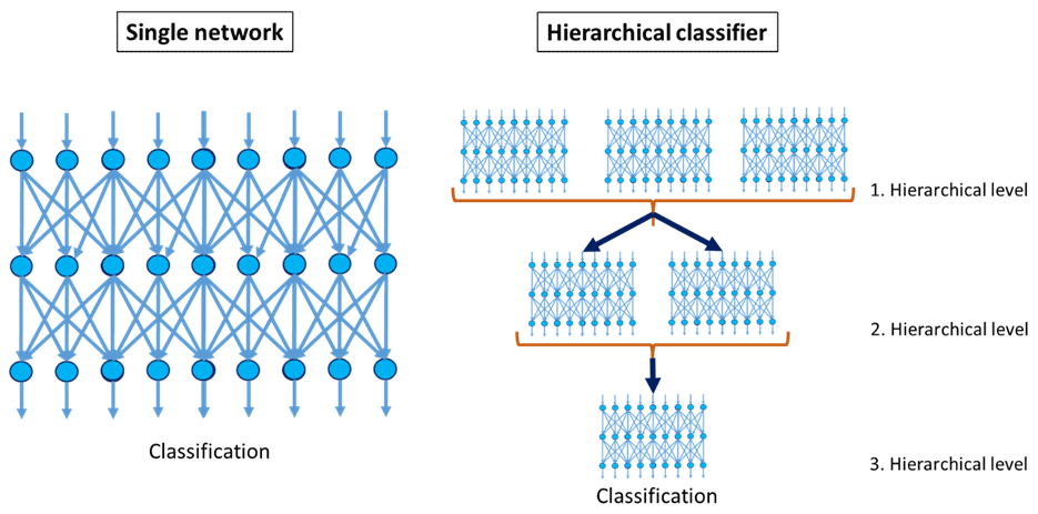
To provide the most accurate visual inspection possible, the detection by a single CNN is currently not sufficient to ensure a reliable control of all solder joints on electrical assemblies. In this context, the results of Schwebig and Tutsch (2020) still show an unsatisfactory number of error slippage and pseudo errors in almost all test datasets, which must be further reduced for use in practice. While some local optimizations of neural networks have already been carried out in previous investigations, the following approach is based on a global expansion of the classification concept. For this purpose, several connected CNNs are combined into an overarching model (Fig. 2). Furthermore, publications have already shown that hierarchical classifiers are particularly effective and well suited to solving categorical problems (Yan et al., 2014; Mao et al., 2016). The goal of this approach is to improve recognition accuracy compared to a single CNN by breaking down the main problem into several minor subproblems. Therefore, each subnetwork is designed to identify certain features (Zheng et al., 2020).
While the single model only consists of one individual network, the hierarchical classifier is made up of several different CNNs. All networks embedded in it can be arranged into multiple hierarchies, whereby the number of levels and networks placed on them is determined by the overall classification task. The classification task must be distributed to the individual subnetworks by grouping the general problem. Thus, the result of this grouping is the mapping of each origin class to defined cluster centers. In this context, it is possible to group the classes either by similarity or by semantics. The formation of the cluster centers is usually based on superordinate features or states, whereby the number of classes per subnetwork should be reduced compared to the origin classes of the overall task. Consequently, the hierarchical grouping and formation of subnetworks are continued until the original class can be determined at certain output points or at the end of the hierarchy (Zheng et al., 2020; Silla and Freitas, 2011).
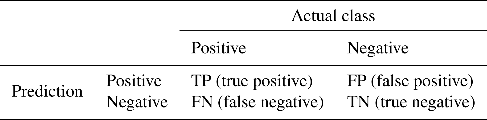
The evaluation metrics accuracy and logarithmic error are used to evaluate the network performance with regard to the training and test data. While the accuracy (refer to Eq. 1) indicates in percentage form how accurate the model performance is compared to the true output, the logarithmic error (refer to Eq. 2) as a loss function describes the error that the network makes in its current training state, taking the respective datasets into account. With multi-classification problems, the logarithmic error of the cross-entropy is used as a measure of the quality via the output of the probability distribution. The cross-entropy is calculated from two probability distributions, the true distribution yi and the estimated distribution p_i. If a learning dataset D={(x1, y1), …, (xi yi)} with M categories is given, the target output yi∈{1, … M in the form of the true distribution is usually a binary one-hot vector expressed with yi∈{0, 1}. In order to make even more detailed statements about the classification performance on unknown data, the F1 score is also included for the test data. The F1 score (refer to Eq. 5) is calculated from the precision (refer to Eq. 3) and the recall (refer to Eq. 4). The precision indicates how many of the predicted classes actually correspond to the true class and the recall shows how many of the actual labels were covered by the correct predictions. This makes it possible to analyze the identification behavior of the network regarding the individual categories further precisely. Since error slippage and pseudo errors play a decisive role in quality assurance, these criteria are also included in the evaluation of the classifier. The pseudo error (refer to Eq. 6) describes as a percentage size how many test data were classified as defective, although there is no defect. On the other hand, the error slip (refer to Eq. 7) represents the worst case in quality assurance, since it reveals the percentage of undetected errors. The formulas and calculation methods for the individual evaluation metrics can be found in the following illustration (Müller and Guido, 2017; Goodfellow et al., 2016; Hope et al., 2018; Raschka and Mirjalili, 2018).
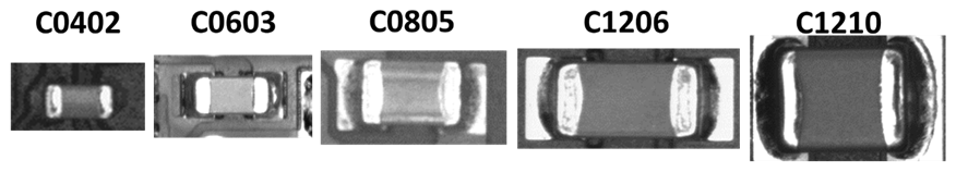
This article is a continuation of Schwebig and Tutsch (2020) and therefore uses both the same component types and test datasets to make the best possible comparison with the single CNN presented in it. Consequently, the results published therein are subsequently used to evaluate the overall performance of the hierarchical classifiers. The component types used for the solder joints in this classification are capacitors and resistors of different sizes (C0402–C1210, R0402/R0603), which are soldered to a printed circuit board as surface-mounted chip parts. Detailed information of the individual components can be found in Schwebig and Tutsch (2020). Figure 2 is an example set of the components and their inspection images.
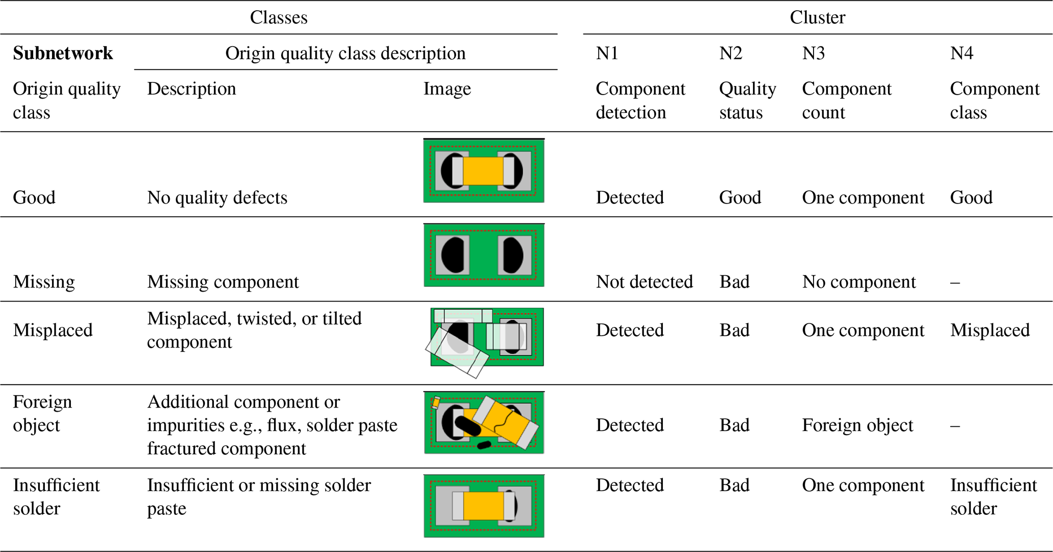
In order to distribute the classification task over several subnetworks, the origin classes specified in the previously mentioned Schwebig and Tutsch (2020) must be grouped into specific clusters. In Schwebig and Tutsch (2020), each class is defined to describe a specific quality status of solder joints on electrical assemblies. The complete defect detection task aims to identify the class of each defect in the image taken by the inspection system. Thus, for the original quality classes for visual inspection of component and solder joint, a distinction is made between the five categories “Good”, “Missing”, “Misplaced”, “Foreign Object”, and “Insufficient Solder”. A precise class definition is given in Table 1.
For the hierarchical classifier, the visual quality inspection of solder joints is divided into several substeps. Each substep includes a CNN that is designed to identify specific properties on component or solder joint. The overarching model consists of two network hierarchies. Accordingly, the first hierarchy consists of three CNNs and initially focuses only on global features. Besides, in the second hierarchy, there is merely a single CNN, whose purpose is for local features and which determines the actual quality class. Each network carries out a classification according to its task, whereas the individual networks do not influence each other.
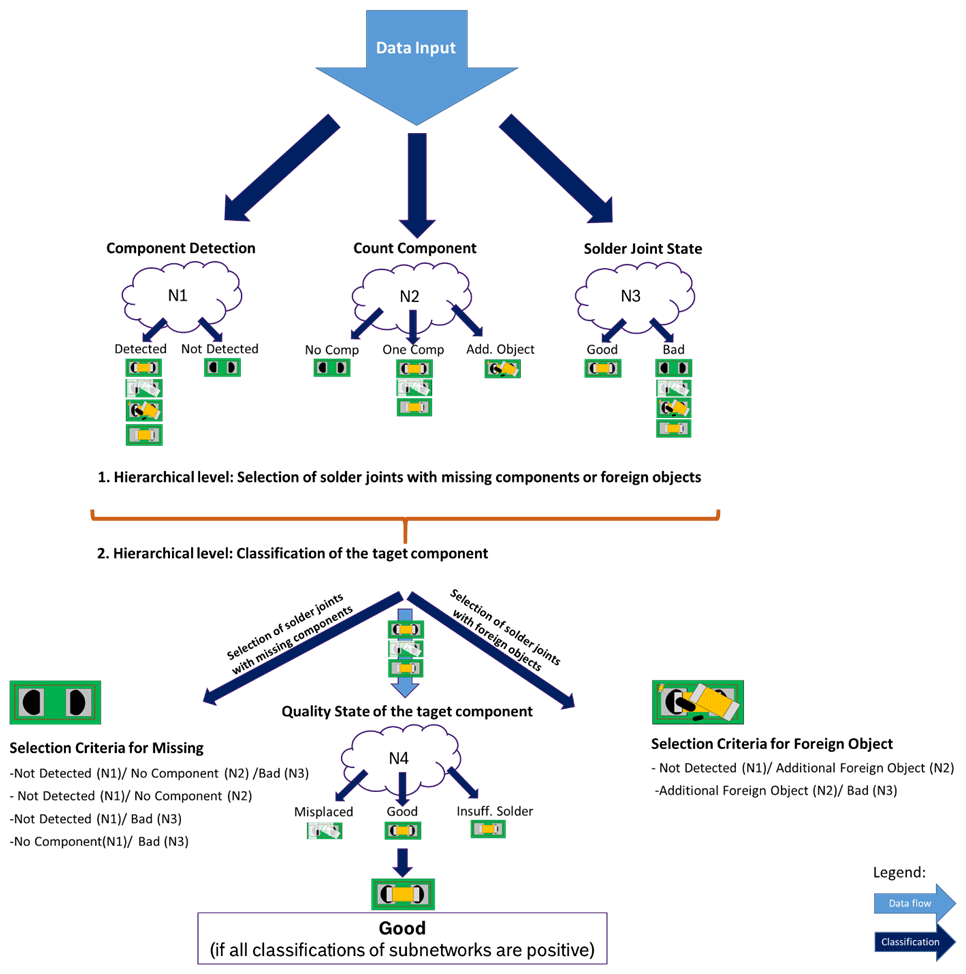
The results of the previous publication, Schwebig and Tutsch (2020), have shown that the quality classes “Good” and “Missing” in particular can be well identified by the neural network. For this reason, the first subnetworks are specifically designed to identify these global features. Thus, the first subnetwork N1 should initially check the presence of the target component at the solder connection point. The distinction is made between the categories “Component Detected” and “Component Not Detected”. While the original category “Missing” only represents the subclass “Component Not Detected”, all other original classes are defined as “Component Detected” because of the presence of components. The second subnetwork N2 makes a general assessment of the solder joint's quality state, distinguishing only between “Good” and “Bad”. Consequently, correctly soldered components are assigned to subclass “Good”, while the error categories characterize subclass “Bad”. With the help of the third sub-CNN, a further detection of the component is carried out and the quantity of components per target position is determined. The task of this network is to designate the number of components or foreign objects and assign them to the classes “No Component”, “One Component”, and “Additional Foreign Object”. Therefore, the focus of this classification is to identify contamination by additional components or foreign bodies. Subclass “No Component” is also characterized by origin class “Missing”. At the same time, irrespective of the quality status, only images of solder joints with the target component present represent subcategory “One Component”. Furthermore, subclass “Additional Foreign Object” is defined by all solder joints that have additional components or foreign objects in addition to the target component. An overview of the structure and the data flow of the hierarchical classifier is given in Fig. 3.
Table 2Classification of the quality classes in the global clusters for the subnetworks (Schwebig and Tutsch, 2020).
The image data pass through the first hierarchical level in a horizontal direction and are forwarded by network N1 via network N2 to network N3. If the absence of a component or the presence of foreign bodies is confirmed by at least two networks after traversing through the first hierarchy, the affected electrical assemblies are sorted out. The aim of this network combination is to detect a missing component or contamination by foreign bodies, so that the final network N4 in the second hierarchical level classifies only solder joints with the target component. Therefore, network N4 is merely trained with data of the target component and finally analyzes the exact quality status of solder joints. It distinguishes only between the origin classes “Good”, “Misplaced”, and “Insufficient Solder”.
Taking into account the classification results of all subnetworks, the overall condition of electrical assemblies should be decided at the end of the second hierarchical level. In this context, the individual assessment of each sub-model is used for the final overall decision. Therefore, only electrical assemblies pass the visual hierarchical network inspection and are assessed as faultless in all instances. The product should merely be transferred to the subsequent process if all classification results are positive. A detailed list of the evaluation criteria for each subnetwork is given in Table 2's classification of the quality classes in the global clusters for the subnetworks (Schwebig and Tutsch, 2020). The detection performance and robustness, particularly in relation to error slippage, will increase due to the solder joints being subjected to multiple visual network inspections. At the same time, the challenge is to keep the number of pseudo errors from increasing due to the accumulation of sequential testing efforts. The aim of the investigations is to develop a universal model for all chip components to inspect the entire electrical assembly. Furthermore, the findings of this work should offer the possibility of subsequent applications to other electronic components.
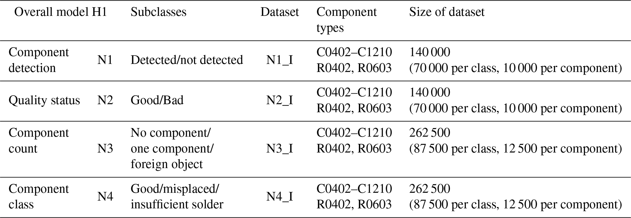
A heterogeneous training dataset with all chip component types is created for each subnetwork. Consequently, these are mixed datasets in which all component types to be inspected are represented. The training datasets were taken directly from production. The number of original image data is determined by the frequency of the corresponding categories or the failure type of the respective component. The validation data used for evaluating the training process and the test data for evaluating the final network performance were randomly selected and split off from the training dataset. In order to generate a balanced training dataset, underrepresented categories were subsequently enriched by augmentation. Therefore, each subclass contains the corresponding components or quality classes in the same number (refer to Schwebig and Tutsch, 2020). While only 10 000 images per component are used for the two-class networks N1 and N2, 12 500 images per component type are available for the three-class networks N3 and N4 due to the higher number of classes and the associated classification complexity. Based on clustering and the results of the previous article (Schwebig and Tutsch, 2020), the training datasets for each subnetwork for the hierarchical overall model H1 were composed as follows.
The hierarchical model is taught by teaching all subnetworks in parallel. For a better comparison, both the network architecture and hyperparameters of the previous investigations in Schwebig and Tutsch (2020) are taken over. Merely the number of classes is modified accordingly for each subnetwork. Every subnetwork is represented by the DenseNet architecture with the additional 5×5 convolutional layer. Hence, both the training and test image data are transferred to the networks in the same size dimensions of bit as in Schwebig and Tutsch (2020). The training duration is 150 epochs for all networks.
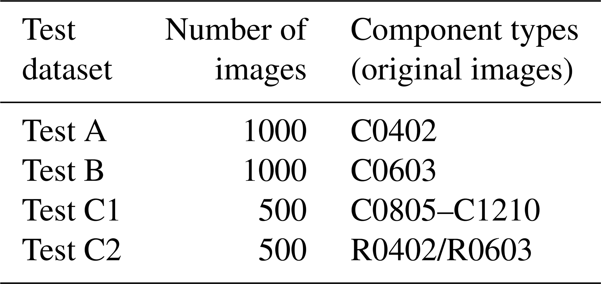
In the actual test phase, the test datasets are presented to the model. In order to achieve the best possible comparability to the single network, the test datasets A–C1 from Schwebig and Tutsch (2020) are used (Table 4). Table 3 provides an overview of the exact composition of the test datasets. To build the overall model H1, all subnetworks are loaded and connected to each other via specific interfaces for data flow. Subsequently, each test dataset is transferred to the hierarchical classifier H1 and goes through the identification process in the defined sequence, while the respective subnetworks carry out their classifications. The data flow continues until the final network N4 for determining the exact quality class is reached or a pre-selection takes place after the first hierarchical level.
Table 4Overview of the used test datasets (Schwebig and Tutsch, 2020).
The detection performance of the overall model is calculated from the partial performances of individual submodels. In order to create the best possible basis for comparison, the evaluation metrics from Schwebig and Tutsch (2020) are applied. For this purpose, accuracy is used as one of the most important measurement parameters in test technology to evaluate the overall recognition performance of neural networks. Consequently, the accuracy is given in the form of a percentage and is intended to evaluate how accurate the network classification is compared to actual classes. In addition, the F1 score is used as an evaluation metric to determine how precisely the individual classes can be identified by each subnetwork. The F1 score can be generated from precision and recall. While the precision indicates that many of the classes predicted as positive are actually positive, the recall analyzes how many positive target outputs match positive predictions.
In this chapter the behavior and performance of the hierarchical concept are examined. For this purpose, the universal model H1 is used, which is based on the classification of chip capacitors C0402–C1210 as well as chip resistors R0402 and R0603. The application objective of the concept is to support optical quality assurance in the real production environment. For this reason, the evaluation of the network performance is carried out exclusively on the unknown test datasets A–C2. First, the results of the individual subnetworks N1–N4 are analyzed. Subsequently, the actual assessment of the overall model is carried out, taking into account the single network from Schwebig and Tutsch (2020).
5.1 Partial results of the hierarchical overall model H1
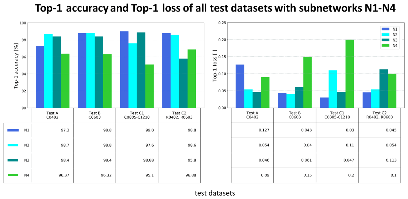
Figure 4 provides an overview of the general recognition performance and the logarithmic error of each submodel N1–N4 with regard to the respective test dataset. All subnetworks can recognize the test datasets A–C1 with an accuracy of over 95 %. For all test datasets, the two-class subnetworks N1 and N2 have the highest detection accuracy. This behavior can be attributed to the grouping of the origin quality classes. Compared to the other subnetworks, networks N1 and N2 only need to distinguish between two global classes. As a result, there are fewer categories and complex features that the networks must classify. Hence, this means that the associated subclasses can easily be determined. It is noticeable that network N4 has the comparatively lowest recognition performance on all test datasets. While network N3 only detects the presence of the target component despite the same number of classes, network N4 must also check the quality states of solder joints in addition to component position. Overall, a correlation between the logarithmic error and the accuracy can be observed in all networks. With a high accuracy, a low loss is monitored, while with a lower accuracy the error grows. Consequently, the associated complexity increases the difficulty of identifying the final quality state, which has a negative effect on detection performance.
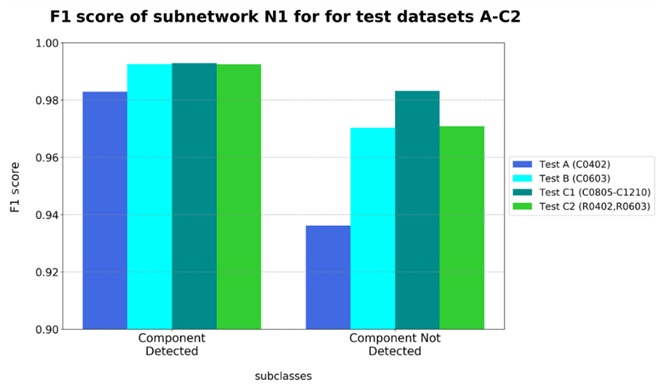
All test datasets of subnetwork N1 have higher F1-score values for class “Component Detected”. Therefore, this category is generally easier to identify for all components. At the same time, a higher overall recognition performance can be observed on larger components of test datasets B and C1 than on the other test datasets (refer to Figs. 4 and 5).
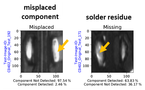
The reason for this behavior can be explained with the help of the respective test images and the corresponding prediction by subnetwork N1. Figure 5 illustrates an example of misclassification by N1 for each category. In particular, extremely misplaced components of origin category “Misplaced” are falsely identified as “Component Not Detected”. This classification tendency always occurs when the largest part of the component is no longer visible in the images of solder joints (refer to Fig. 6 left). Since connecting surfaces are completely exposed in the case of a large component offset, the features of empty solder joints dominate for the network. Consequently, the affected images are classified as “Component Not Detected”. For larger components, this type of offset is less common due to their size. The reason for this is that with increasing component size a major part of the image shows only the component. As a result, test datasets B and C1 have a higher F1 score than test dataset A with the small capacitors C0402. Since this recognition problem can be increasingly observed with network N1, network N3 has a higher accuracy despite a similar classification task. In the case of solder joints with a missing component, solder residues on connection points seem to be responsible for wrong decisions made by the network (refer to Fig. 6 right). Depending on the amount and shape of solder, the network identifies parts of a component body, whereby the affected image is assigned to category “Component Detected”. Since most images of origin class “Missing” show relatively few solder residues on the free connecting surfaces, this behavior can be attributed to an insufficient number of training data with this feature.
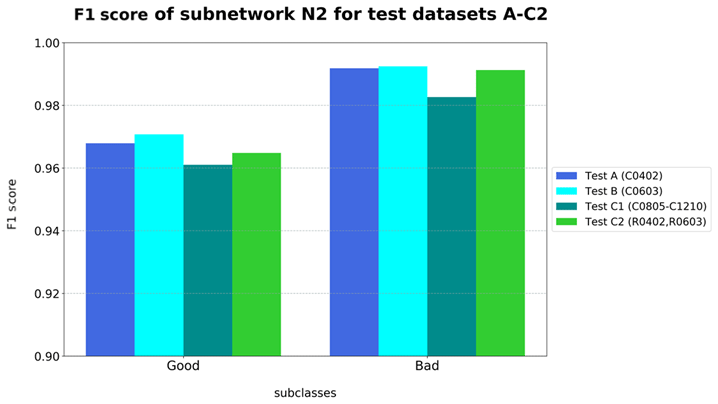
Category “Bad” of network N2 has the greatest detection accuracy for all test datasets (refer to Fig. 7). It is noteworthy that test datasets A, B, and C2 have a higher identification performance than test dataset C1 with larger capacitors. For smaller components and their connection points, faults occur with a higher frequency due to manufacturing processes. Consequently, more data of failure types can be obtained from production. For this reason, the behavior is due to the higher proportion of original images in the training datasets and the associated data variance (refer to Schwebig and Tutsch, 2020).
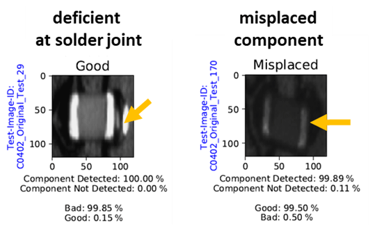
The misclassifications by network N2 can mainly be found on solder joints whose general quality is close to the limit of tolerance between sufficient and insufficient. In particular, this can be observed in the case of connection points, which meet all quality criteria in accordance with the specifications but nevertheless have a slight deviation in terms of component position or shape of solder joint (refer to Fig. 8 left). If the network identifies the flaw as the dominant feature, the actually defect-free solder joint is classified as insufficient. In this context, a similar classification behavior can also be observed in the images of the individual error types. In the event that the target component is in the correct position despite a defect or failure, the affected images of solder joints are increasingly assigned to class “Good” (refer to Fig. 8 right).
Classes “No Objects” and “One Component” of network N3 show a similarly high detection performance due to the comparable F1 score (refer to Fig. 9), despite category “Additional Foreign Object” having a relatively low level of identifiability. It is especially remarkable that the resistors of test dataset C2 have a lower accuracy in all categories than the other test datasets.
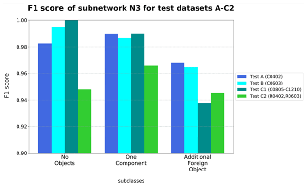
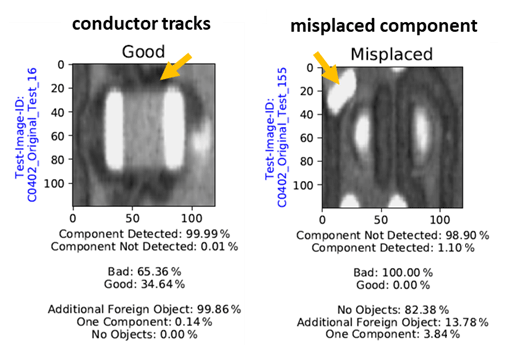
The reason for the comparably poor identification performance of the resistors lies primarily in the fact that solder joints with additional conductor tracks in the surrounding area are increasingly classified as “Additional Foreign Object”. Since the PCB usually has a homogeneous surface near the connection points, the network is increasingly aligned to this physical appearance. Hence, there is an assumption that the network identifies the conductor tracks as foreign bodies, which influences the decision as the dominant feature (refer to Fig. 10). In particular, test dataset C2 has an enhanced number of conductor tracks near the connection surfaces. Consequently, this feature is responsible for the fact that resistors and subcategory “Additional Foreign Object” have a comparatively lower detection performance (refer to Fig. 9). Test dataset C2 was captured from a different product family. For this reason, the PCB design varies significantly from that of the other test datasets.
As already observed on network N1, network N3 also classifies extremely misplaced components as “No Objects” (refer to Fig. 6). For this reason, solder joints with lots of misplaced components are removed from the further evaluation process by preselection after the first hierarchical level. In this context, it is sufficient if two of three networks detect the absence of a component or a contamination at the solder joint.
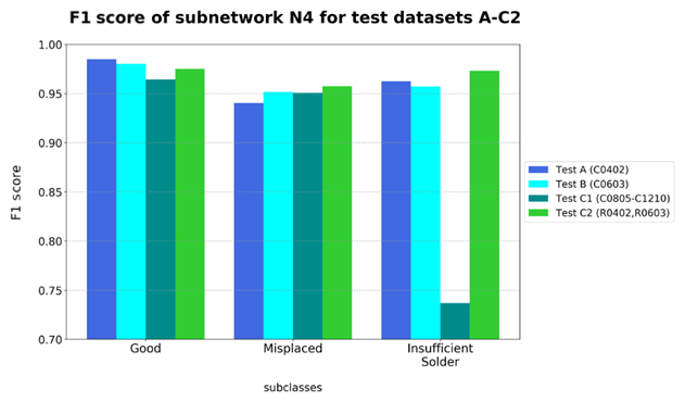
The F1-score values of network N4 show that the overall classification performance is highest for class “Good”, while the other categories have a lower detection accuracy (Fig. 11). As already examined in Schwebig and Tutsch (2020), the challenge for neural networks is to correctly classify solder joints with features of different quality classes. In particular, misclassification occurs when there is an additional misplaced component in addition to the actual category. The test images show that the network frequently confuses the classes “Misplaced” and “Insufficient Solder” with each other if they contain features of the other class as well (refer to Fig. 12). At the same time, sufficient solder joints with slight deviations are already assigned to a defect class. The features that dominate for the network determine the final decision when detecting the quality classes.

It is noticeable that test dataset C1 with larger capacitors has the lowest detection accuracy in class “Insufficient Solder”. The reason for this is due to the low proportion of original component images for this category. Since this error type is less common for large components, fewer image data are available in this context (refer to Schwebig and Tutsch, 2020).
5.2 Overall results of the hierarchical model H1
After running through the final subnetwork N4 of the second hierarchy, an overall decision is made based on prediction results of all subnetworks about the final quality status of electrical assemblies. In order to enable a better evaluation of the classification results, the detection outputs of this hierarchical model H1 are compared with that of the equivalent single network from Schwebig and Tutsch (2020) (Table 5). The single network is a five-class model with the same network architecture, which was trained with training dataset G to identify the same component types and quality classes. In this context, single model means that the origin classes “Good”, “Missing”, “Misplaced”, and “Insufficient Solder” are determined by only one CNN. The following table shows the total recognition performance of classifiers on respective test datasets, as well as percentage of error slippage and pseudo errors.
Table 5Overall results of the hierarchical model H1.
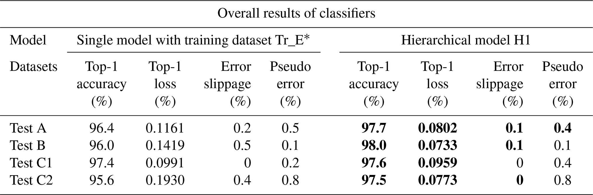
* Refer to Schwebig and Tutsch (2020). Legend: the values marked in bold indicate where an improvement has been achieved by the hierarchical classifier.
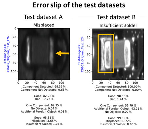
A comparison of the overall classification results shows that the general detection performance on all test datasets can be increased with the hierarchical approach. In addition, the logarithmic error of the loss function is reduced. Due to the multiple classification, the error slippage could be reduced by more than half. Out of 3000 test datasets, only three classified images are subject to an undetected defect. These are solder joints, the quality of which is near the tolerance limit to distinguish between sufficient or insufficient quality. Figure 13 shows the affected images of different failure types that were not detected by the hierarchical model. Although capacitor C0402 of test dataset A is still located at both solder joints, it shows an offset in the left direction. Since the features for “Good” dominate due to the combination of sufficient solder joints and component position, there is an error slippage despite multiple network classifications. In the case of test dataset B, the error slippage can be found in class “Insufficient Solder”. Here, the target component was correctly placed but has an insufficient solder joint on the left-hand side. Since the “Good” features are predominant in their representation for all subnetworks, these images are classified incorrectly.
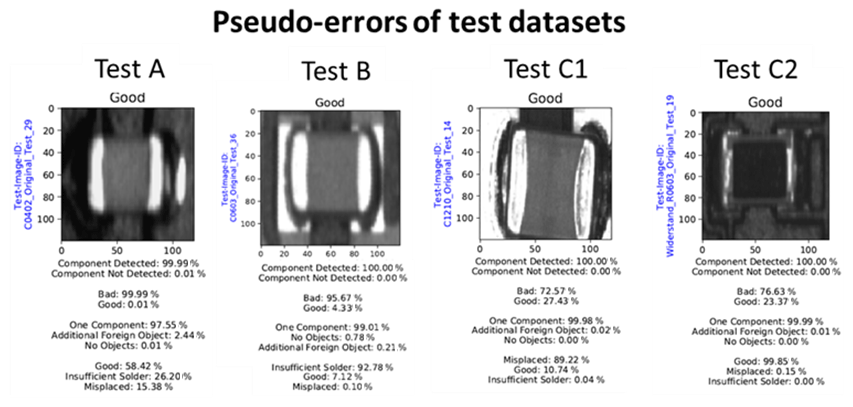
Despite multiple testings by the individual subnetworks, the pseudo error occurrences did not additionally increase except for test dataset C1. The higher number of pseudo errors on larger components is due to the comparatively lower proportion of original images in training data (refer to Schwebig and Tutsch, 2020). By distributing the overall classification task across various subnetworks, the misclassification value is kept at a low level (refer to Fig. 13). It is observed that the networks increasingly assign solder joints with additional conductor tracks in the surrounding area to a wrong category. For this reason, the general pseudo error occurrence is mainly due to this feature. In addition, further pseudo errors were found with electrical connection points that show either a slight component offset or a discreetly less pronounced solder joint. If a network assigns a higher relevance to one of these features that deviate from the target, an incorrect classification takes place (Fig. 14).
The increased accuracy and robustness against error slippage can be explained by a higher testing effort of solder joints by individual subnetworks. Despite multiple inspections, the number of pseudo errors has not been increased. The clustering into global and local features reduces the complexity and distributes it to individual subnetworks. After passage of the first hierarchy, a preliminary decision is already made by selecting empty or contaminated solder joints. The aim of this selection is that only solder connections with the target component are transferred to the last subnetwork N4. In advance, this prevents insufficient solder joints with these failure types from not being recognized. As a result, an electrical assembly is only considered to be fault-free if all four subnetworks confirm the sufficient quality status of all solder connections. Consequently, this flow minimizes the probability that errors will remain undetected. Therefore, the final decision is no longer dependent on just one neural network but is based on a multi-eye principle of a hierarchical model.
While most optical inspection systems can only determine the very existence of an error, the use of convolutional neural networks offers the possibility of identifying the exact error details. The aspect shows a decisive advantage with regard to the use of a deep learning concept in the area of optical quality assurance. This article introduces a hierarchical CNN classifier for analyzing solder joints on electrical assemblies and demonstrates its higher recognition performance compared to a single CNN. In particular, error slippage and pseudo errors can be compensated by multiple visual inspections, which increases the robustness of the overall model. The advantage of a hierarchical network is that it is able to solve difficult tasks by dividing the overall classification task into several simpler subtasks. The effort of handling the problem is distributed among various subnetworks according to difficulty. In the context of this work, the same network architecture is used for all subnetworks. Alternatively, an individual network architecture can be used for each subproblem, which is specially adapted to its classification task. The investigations of previous publications have shown that particularly high detection results can be achieved if training datasets are explicitly geared to the respective component types. In regard of future work, component types of similar size and appearance will be combined in training datasets for each subnetwork, with the aim of further increasing the recognition performance of the hierarchical classifier.
The datasets that we used cannot made publicly available on a public repository. The data used was provided by Robert Bosch GmbH as part of a confidentiality agreement.
AIMS developed the concept and the procedure, implemented the network architecture, carried out the investigation, visualized the results and wrote the original draft of the paper. RT visualized the results, reviewed and edited the paper.
The authors declare that they have no conflict of interest.
This work was supported by Robert Bosch Elektronik GmbH Salzgitter in Germany and the Technische Universität Braunschweig.
This research has been supported by the Technische Universität Braunschweig (grant no. G2020-5).
This open-access publication was funded
by the Technische Universität Braunschweig.
This paper was edited by Rosario Morello and reviewed by two anonymous referees.
Berger, M.: Test- und Prüfverfahren in der Elektronikfertigung: Vom Arbeitsprinzip bis Design-for-Test-Regeln, VDE-Verlag, Berlin, 250 pp., 2012.
Combet, C. and Chang, M.-M.: 01005 Assembly, the AOI route to optimizing yield, Vi TECHNOLOGY, available at: https://smtnet.com/library/files/upload/01005Assembly.pdf (last access: May 2020), 2009.
Goodfellow, I., Bengio, Y., and Courville, A.: Deep learning, MIT Press, Cambridge, Massachusetts, London, UK, 1785 pp., 2016.
Hope, T., Resheff, Y. S., and Lieder, I.: Einführung in TensorFlow: Deep-Learning-Systeme programmieren, trainieren, skalieren und deployen, Safari Tech Books Online, O'Reilly, Heidelberg, 224 pp., 2018.
Mao, X., Hijazi, S., Casas, R., Kaul, P., Kumar, R., and Rowen, C.: Hierarchical CNN for traffic sign recognition, in: IEEE Intelligent Vehicles Symposium (IV), Gothenburg, 130–135, https://doi.org/10.1109/IVS.2016.7535376, 2016.
Müller, A. C. and Guido, S.: Einführung in Machine Learning mit Python: Praxiswissen Data Science, O'Reilly, Heidelberg, 362 pp., 2017.
Niemann, J., Härter, S., Kästle, C., and Franke, J.: Challenges of the Miniaturization in the Electronics Production on the example of 01005 Components, in: IEEE International Conference on Computer Vision (ICCV 2015), Santiago, Chile, 113–123, https://doi.org/10.1007/978-3-662-54441-9_12, 2017.
Raschka, S. and Mirjalili, V.: Machine Learning mit Python und Scikit-Learn und TensorFlow: Das umfassende Praxis-Handbuch für Data Science, Deep Learning und Predictive Analytics, 2. aktualisierte und erweiterte Auflage, mitp, Frechen, 577 pp., 2018.
Schwebig, A. I. M. and Tutsch, R.: Compilation of training datasets for use of convolutional neural networks supporting automatic inspection processes in industry 4.0 based electronic manufacturing, J. Sens. Sens. Syst., 9, 167–178, https://doi.org/10.5194/jsss-9-167-2020, 2020.
Silla, C. N. and Freitas, A. A.: A survey of hierarchical classification across different application domains, Data Min. Knowl. Disc., 22, 31–72, https://doi.org/10.1007/s10618-010-0175-9, 2011.
Yan, Z., Zhang, H., Piramuthu, R., Jagadeesh, V., DeCoste, D., Wei, D., and Yu, Y.: HD-CNN: Hierarchical Deep Convolutional Neural Network for Large Scale Visual Recognition, available at preprint: http://arxiv.org/pdf/1410.0736v4 (last access: May 2020), 2014.
Zheng, Y., Fan, J., Zhang, J., and Gao, X.: Discriminative Fast Hierarchical Learning for Multiclass Image Classification, IEEE T. Neural Netw. Learn. Syst., 31, 2779–2790, https://doi.org/10.1109/TNNLS.2019.2948881, 2020.
- Abstract
- Introduction
- Hierarchy formation of CNNs and data flow
- Compilation of training datasets for each subnetwork
- Network architecture and training details
- Outcomes and results of the hierarchical overall model
- Conclusion
- Data availability
- Author contributions
- Competing interests
- Acknowledgements
- Financial support
- Review statement
- References