the Creative Commons Attribution 4.0 License.
the Creative Commons Attribution 4.0 License.
 | 16 Jun 2022
Acceptance and reverification testing for industrial computed tomography – a simulative study on geometrical misalignments
Florian Wohlgemuth
Ingomar Schmidt
Wolfgang Kimmig
Karl Dietrich Imkamp
Acceptance and reverification testing for industrial X-ray computed tomography (CT) is described in different standards (E DIN EN ISO 10360-11:2021-04, 2021; VDI/VDE 2630 Blatt 1.3, 2011; ASME B89.4.23-2020, 2020). The characterisation and testing of CT system performance are often achieved with test artefacts containing spheres. This simulative study characterises the influence of different geometrical error sources – or geometrical misalignments – on these sphere measurements. The two measurands on which this study focuses are the sphere centre-to-centre distances and the sphere probing form errors.
One difference between the current draft of the ISO 10360-11 standard (E DIN EN ISO 10360-11:2021-04, 2021) and the VDI/VDE standard 2630 part 1.3 (VDI/VDE 2630 Blatt 1.3, 2011) as well as the ASME standard B89.4.23 (ASME B89.4.23-2020, 2020) are the differences for the sphere centre-to-centre distances that need to be measured. The VDI/VDE standard and the ASME standard require measurements of these kinds of distances of up to 66 % of the possible maximum distance within the measurement volume, while the ISO draft asks for measurements of up to 85 % of the possible maximum distance. This requirement needs to be considered in connection with the maximum permissible error (MPE) specification for these sphere distance measurements. This MPE should be specified as a linear function of the nominal distance or a constant value or a combination thereof (compare definition 9.2 of ISO 10360-1:2000 + Cor.1:2002 (DIN EN ISO 10360-1:2003-07, 2003)), and thus, the linearity of the length-dependent maximum measurement error of the sphere distance measurements is of interest. This simulative study inspects to what extent this linearity can be observed for CT measurements under the influence of different geometric errors. Further, the question is whether measurement lengths above 66 % necessitate a change in the MPE specification. Thus, an automatic identification of cases that might affect the MPE specification is proposed, and these cases are inspected manually.
A second aspect of this study is the impact of geometrical misalignments on the probing form errors of a measured sphere. The probing form error also needs to be specified. Thus, whether and how it is influenced by the misalignments is also of interest.
Based on our simulations, we conclude that probing form errors and sphere centre-to-centre distances of up to 66 % of the maximum possible measurement length within the measurement volume are sufficient for acceptance testing concerning geometrical misalignments – each geometrical misalignment can be detected well with at least one of these two measurands.
- Article
(6207 KB) - Full-text XML
- Companion paper
- BibTeX
- EndNote


Acceptance and reverification testing for industrial X-ray computed tomography (CT) is important for users and manufacturers alike as it is used to test technical specifications that are contractually guaranteed. The testing procedure is described in different standards (E DIN EN ISO 10360-11:2021-04, 2021; VDI/VDE 2630 Blatt 1.3, 2011; ASME B89.4.23-2020, 2020). The characterisation and testing of CT system performance are often achieved with test artefacts containing spheres. Measurands in acceptance testing that we inspect in this paper are the errors in centre-to-centre distances of the spheres (SD errors) as well as the sphere probing form errors. This simulative study characterises the influence of different geometrical misalignments of the CT acquisition geometry on these sphere measurements. One difference between the current draft of the ISO 10360-11 standard (E DIN EN ISO 10360-11:2021-04, 2021) and the VDI/VDE standard 2630 part 1.3 (VDI/VDE 2630 Blatt 1.3, 2011) as well as the ASME standard B89.4.23 (ASME B89.4.23-2020, 2020) are the differences for the sphere centre-to-centre distances that need to be measured. Both the VDI/VDE standard and the ASME standard require measurements of up to 66 % of the possible maximum distance within the measurement volume, while the ISO 10360-11 draft asks for measurements of longer distances (current draft: measurements of up to 85 %). In the usual case of a cylindrical measurement volume, the maximum distance within the measurement volume is the diagonal. The requirement to measure up until certain lengths needs to be considered in connection with the maximum permissible error (MPE) specification for these sphere distance measurements. This MPE should be specified as a linear function of the nominal distance or a constant value or a combination thereof (compare definition 9.2 of ISO 10360-1 (DIN EN ISO 10360-1:2003-07, 2003)), and thus, the linearity of the length-dependent maximum measurement error of the sphere distance measurements is of interest. This simulative study inspects to what extent linearity can be observed for CT measurements under the influence of different geometric errors. Further, the question is whether measurement lengths above 66 % necessitate a change in the MPE specification. Thus, an automatic identification of cases that might affect the MPE specification is proposed, and these cases are inspected manually.
A second aspect of this study is the impact of geometrical misalignments on the probing form errors of a measured sphere. The probing form error does also need to be specified and can also indicate geometrical misalignments. Thus, whether and how it is influenced by the misalignments is also of interest. Generally, it will suffice that either probing form errors or sphere centre-to-centre distances are sensitive to a specific geometric misalignment.
Similar work has been performed by Muralikrishnan et al. (2019a, b, c) and Jaganmohan et al. (2020). The difference between that study and the work presented here is that the study by Muralikrishnan et al. (2019a) employs a self-developed geometric forward- backward projection simulation of the sphere centre points, while we use the radiographic simulator aRTist 2 by the German Federal Institute for Materials Research and Testing (BAM) (see, for example, Bellon et al., 2012) and simulate realistically sized spheres. The radiographic approach also means that our simulations produce projection data which are subsequently processed with volume reconstruction and surface point determination the same way real CT data are processed. A further difference is that Muralikrishnan et al. (2019a, b, c) and Jaganmohan et al. (2020) had the goal of finding the most sensitive measurement distances for different single geometric errors, while we want to analyse the distribution of the sphere centre-to-centre distance errors with respect to the nominal distance and inspect probing form errors. Another extension in comparison the work of Muralikrishnan et al. (2019a, b, c) and Jaganmohan et al. (2020) is that in our analysis, we want to include simulations with combinations of multiple geometric misalignments as real CT systems will also show a combination of these.
The MPE can be specified as a linear function of the measurement length, a constant value or the minimum of both. In agreement with VDI/VDE 2630 Blatt 1.3 (2011), we disregard the option of constant values for SD errors in dimensional computed tomography. It is well known that translations of rotary table, source and detector in the beam direction lead to scaling errors that increase linearly with the nominal length (as shown by simulation results in Sect. 4.1). Assuming a linear MPE specification, the decision as to whether long sphere distances need to be measured depends on how the maximum errors in these distance measurements increase with the nominal sphere distance. We can imagine four different patterns for the SD errors (compare Fig. 1). First, they can increase linearly with the sphere distance. Second, they can increase roughly linearly with the sphere distance, meaning that there are two parallel linear functions within which all data points lie. Third, they can increase with the nominal distance less than a linear function would (e.g. with a square-root behaviour), and fourth, they can increase more than a linear function would (e.g. with a parabolic increase). Of these four cases, only the case of “more than linear” increase needs to be considered relevant in the context of the MPE specification, as an MPE based on data for lower lengths might not be valid any more at long lengths. This will not happen in the other three cases.

Figure 1Four different patterns for the SD errors can be imagined. The pattern in plot (a) illustrates strictly linear behaviour, indicated by a correlation coefficient of ρ=1. The pattern in plot (b) illustrates a behaviour that is roughly linear in the sense that there are two parallel linear functions within which all data points lie. The pattern in plot (c) illustrates an increase that is less than linear; i.e., the increase of the measurement deviation with the nominal length is less than linear. The pattern in plot (d) indicates more than linear behaviour. This latter behaviour is the only one we would deem relevant for the MPE specification as an MPE limit constructed using points up to a certain percentage might easily be exceeded by points at a higher percentage. The plots show that while the correlation coefficient ρ can detect strictly linear behaviour, it is not sufficient for deciding whether or not a given pattern would be relevant regarding the MPE specification.
In the following, we will often use the Pearson correlation coefficient ρ (or the square root of the coefficient of determination R2 of a linear fit to the data; see Fahrmeir et al., 2009) to gauge linearity. While a value of |ρ|≈1 indicates linear behaviour, a value below 1 does not allow for any statement about the kind of non-linearity the data exhibit. Therefore, any value clearly different from 1 does not allow for any conclusion on whether the underlying data would be relevant in the context of a linear MPE specification or not. Therefore, we propose a further analysis method in Sect. 5 which provides an automated criterion for cases with |ρ|≠1.
Section 3.1 describes the simulation parameters and geometry, including the geometric misalignments that can be simulated. Section 3.2 describes the artefact geometry that is used for this study. Section 3.3 describes the data processing after the radiographic simulation.
3.1 Simulation parameters and geometry
For the simulation, we used aRTist 2 by the German Federal Institute for Materials Research and Testing (BAM) (see, for example, Bellon et al., 2012) in version 2.10.0. To minimise the influence of other error sources, the simulations are monochromatic (200 keV), without scatter, and the detector is perfectly linear with a maximum grey value of 60 000 at free beam. The simulation artefact material is set to aluminium. The detector of the acquisition setup has a pixel pitch and unsharpness of 0.4 mm and is noise-free. The detector is positioned 1000 mm from the point source and the object at 250 mm, resulting in a magnification of 4. The detector is 600 mm wide and 500 mm high (equivalent to 1500 pixels × 1250 pixels). The resulting half-cone beam angle is 16.7∘. A total of 1500 projections on a regular circle trajectory are simulated. The measurement volume, i.e., the cylinder whose content is completely projected onto the detector in all projections, has a diameter of 121.27 and a height of 113.62 mm. Its diagonal (the maximum distance within the cylindrical measurement volume) is 166.18 mm long. The STL (Standard Triangle Language file format) model of the simulation artefact is positioned with its bounding box centre at mm and with a distance of 250 mm to the source along the z axis (see Fig. 2 for the coordinate system definition). In a real CT, the rotary table should not be projected onto the detector. The pivot point of the rotation axis is therefore located 77.125 mm below the central beam axis (translated downwards in the negative y direction). This will become relevant when misalignments are considered. The acquisition geometry is illustrated in Fig. 2.
aRTist 2 can simulate projection-wise geometric errors of the acquisition geometry (compare, for example, Wohlgemuth et al., 2018, 2020). The original implementation of aRTist 2 was modified slightly for the purpose of this study. The following modifications are possible for each projection (in this order):
-
Detector position and orientation, source position and rotation axis position are modified (with respect to their undistorted value) according to values for this projection from an input file. If vud is the undistorted (nominal) parameter value (3D vector), then the parameter value v(j) for projection j results from a displacement value δ(j) according to
-
The value for the direction of the rotation axis for this projection (again from an input file) is applied. The rotation axis direction is encoded as a 3D unit vector in aRTist; thus, the input file contains one such unit vector n(j) for each projection j which is applied in this step.
-
The measurement object is translated and rotated to account for the movement of the rotation axis (the connection between measurement object and rotary table is assumed to be rigid). This means that the translation of the rotation axis position between projection j−1 and j is applied also to the object and that the object is then rotated to account for the different orientation between rotation axis direction n(j−1) from projection j−1 and projection axis direction n(j) from projection j.
-
After image acquisition, the object is rotated by the angular increment value for this projection (again from an input file) around the current rotation axis with direction n(j) and position for projection j.
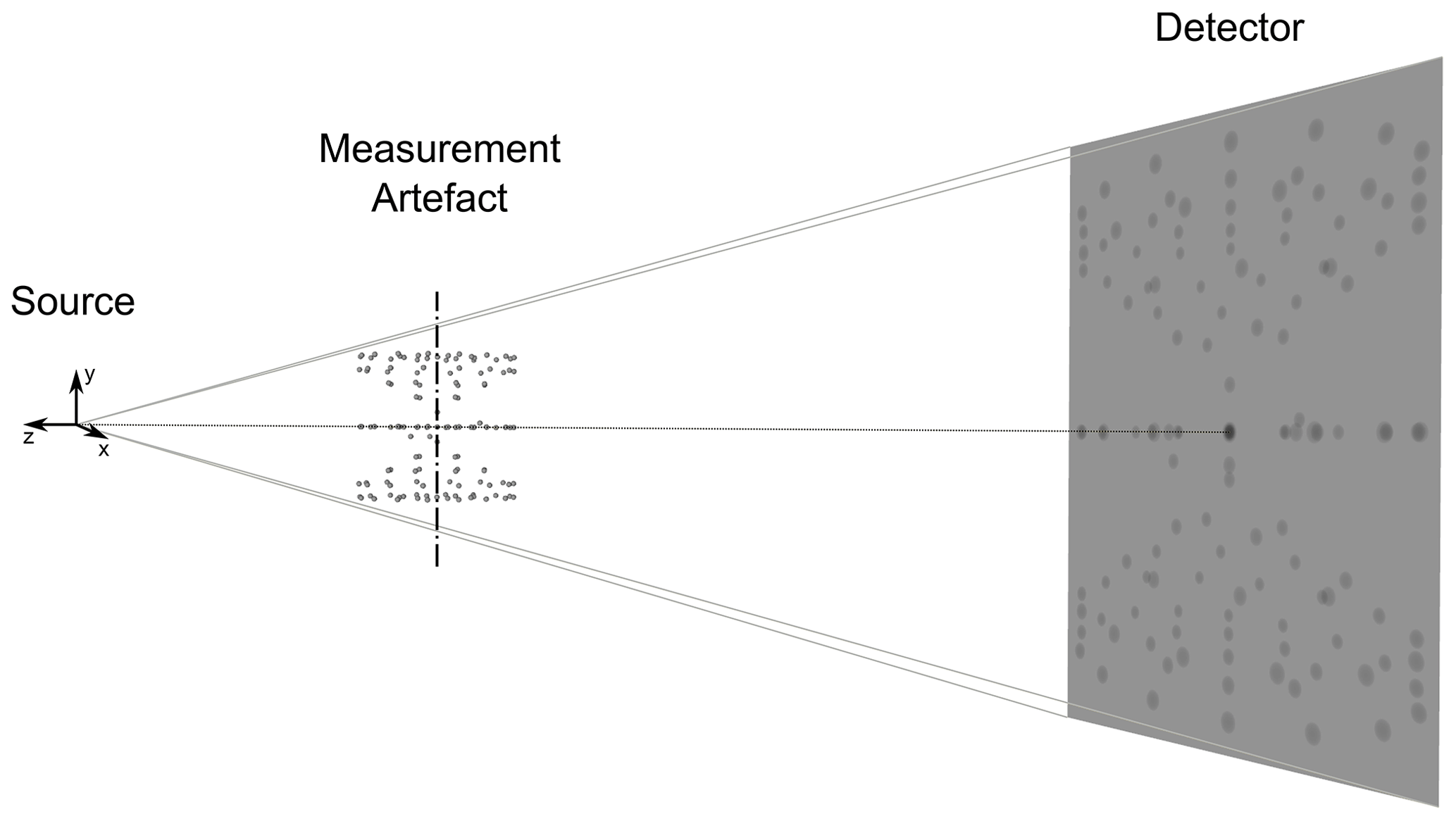
Figure 2Illustration of the acquisition geometry along with the coordinate system used. The negative z axis is the beam direction, the y axis is parallel to the axis of rotation and the x axis is the second direction along the detector (besides the y axis). The rotation axis almost coincides with the axis of the measurement artefact and has its pivot point below the beam cone to model a real CT system realistically. The source is an isotropic point source.
These modifications are used to represent actual possible geometrical misalignments of an industrial CT, described in the following. Without reference to the specific machine performance of a specific CT, it is unclear what good numerical values for these geometrical misalignments are. We used estimated values as described below, but we did also vary the numerical values during the study (see Sect. 4).
-
Detector position perpendicular to central beam axis (x and y axis). For the detector translation perpendicular to the central beam axis (x and y direction), we assume a maximum error of 2 mm.
-
Detector position along beam axis (z axis). A detector translation in the beam direction can be detected as a scaling error. We assume that one of the most simple calibration procedures is to use two spheres with calibrated distance and project these onto the detector. The distance between the projected sphere centres divided by the calibrated distance can be used to determine the magnification. If we assume that the magnification is M=4, the calibrated distance is 10 mm ± 1 µm and the centre-to-centre distance determination on the projection is possible with half pixel pitch accuracy, then the relative error of the source detector distance is around . Assuming that this is the uncertainty in source–detector distance, this translates into a maximum detector misalignment in beam direction (z direction) of 3.75 mm.
-
Detector orientation. With a simple spirit level, a measurement accuracy of 0.057∘ can be achieved. Therefore, we assume a maximum detector tilt in all directions of this measurement accuracy.
-
Source position. For the translation perpendicular to the beam axis (x and y axis), we assume – as with the detector – a maximum error of 2 mm. The beam axis (z axis) translation induces – as with the detector – a scaling error. With the same estimation as for the detector, we used a maximum error of 0.65 mm in the beam direction.
-
Rotation axis tilt. Like Muralikrishnan et al. (2019a) and Muralikrishnan et al. (2019b), we use a maximum error of 0.2∘ tilt in all Cartesian directions.
-
Rotation axis position. For the beam direction (z axis), a similar argument as for the source position holds, and the maximum error we assumed is thus also 0.65 mm.
-
Dynamic rotation axis errors. The dynamic rotation axis errors are the dynamic errors of the rotary table. The rotary table has different errors in its movement which can all depend on the rotation angle. For translations, we model both a dynamic shift in height (y axis) and a translation in radial (x–z plane) direction. For the direction of the rotation axis, a wobble is implemented. This wobble is in radial direction and is characterised by its angle with the tilted rotation axis. All dynamic errors depend on the angular position in the same form given by Eq. (2). In this equation, 𝒩 is a normalisation factor given by max(fdyn), φ is the angular step angle of the projection and Φk denotes phase angles. For each single projection step, the amplitude of each dynamic misalignment is modulated by multiplication with this factor fdyn. The idea behind this approach is to characterise the dynamic effects by a Fourier series (truncated and with equal amplitudes for all frequencies). The truncation at k=10 was motivated by the works of Muralikrishnan et al. (2019a) and Muralikrishnan et al. (2019b). The inclusion of k=0.5 is motivated technically as rotary tables often have deviations which repeat every second revolution. This two-revolution period is the reason for corresponding testing requirements in technical standards concerning rotary tables (e.g. VDI/VDE 2617 Part 4 Sect. 3.4 (VDI/VDE 2617 Blatt 4, 2006) or ISO 10360-3 Sect. 5.3 (DIN EN ISO 10360-3:2000-08, 2000)). For the selection of the phase angles Φk, see Sect. 4.2.
3.2 Simulation artefact
An often used standard for acceptance and reverification testing is the so-called multi-sphere standard (see, for example, Fig. 6.9.b of Carmignato et al., 2018). In the work by Muralikrishnan et al. (2019a, b, c) and Jaganmohan et al. (2020) a 125-sphere standard consisting of five layers of 25 spheres was used. For this work, we constructed a CAD model combining both ideas. It uses spheres of 4 mm diameter. There are three layers of 25 spheres, each having a centre sphere, a ring of 8 and a larger ring of 16 spheres around this central sphere, equally spaced at radii of 28.25 and 56.5 mm. The layers are at a height of −10, 42 and 94 mm. Further, the model contains two multi-sphere standards with 27 spheres each, one of which is upside down. Their base level is 0 and 84 mm respectively. Further, three additional spheres are added close to the central layer to break spherical symmetry. The total number of spheres in the artefact is 132 (symmetry-breaking spheres included).
Figure 3 shows the simulation artefact described and Fig. 4 a histogram of the sphere distances within the artefact. There is a sufficient number of long sphere distances above 66 %. Accounting for the fact that real spheres have a diameter (and, thus, a measurement distance of 100 % is physically impossible) and that further, geometrical misalignments can easily lead to outer spheres leaving the projections if they are too close to the perimeter (thus causing artefacts), the embodied lengths extend to a reasonable maximum of what can still be measured.

Figure 3Simulation artefact (nominal positions of the sphere centres) consisting of three layers of 25 spheres in red (inspired by Muralikrishnan et al., 2019a, b, c and Jaganmohan et al., 2020) and two multi-sphere standards with 27 spheres (in blue). There are further symmetry-breaking spheres indicated by stars.
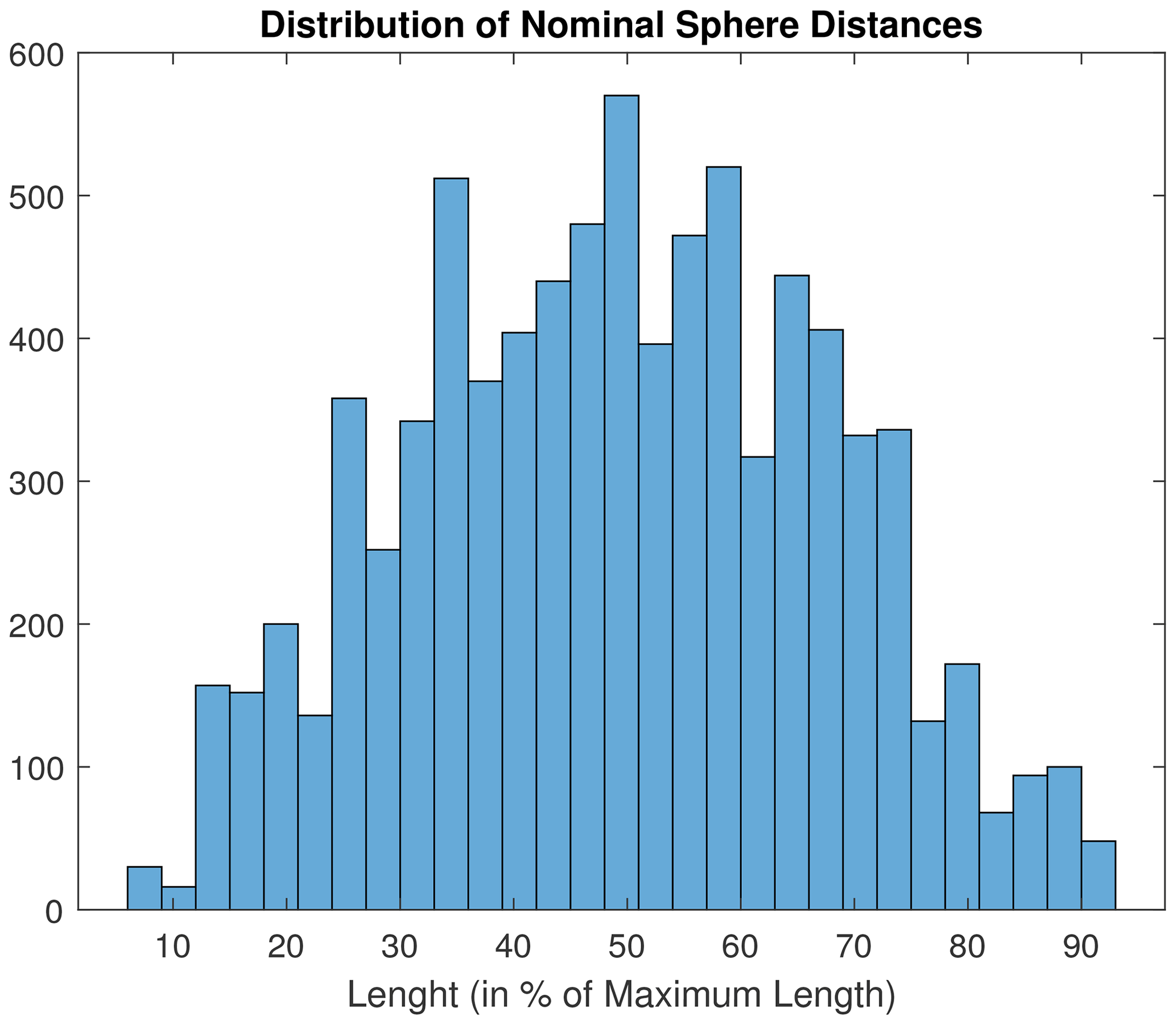
Figure 4Distribution of the nominal sphere centre-to-centre distances in the simulation artefact. While the range of ≈35 % to 65 % is represented by more lengths, there are still a considerable number of short and long lengths within the artefact.
3.3 Reconstruction and dimensional evaluation
The simulation in aRTist 2 results in flat-field-corrected projections. To reconstruct these, the ASTRA Toolbox (version 1.9.0. dev11 in MATLAB R2021a; see van Aarle et al., 2016, 2015) was used. For dimensional evaluation, the reconstructed volumes were batch processed using Volume Graphics GmbH (Heidelberg, Germany) VGSTUDIO MAX version 3.4.0 (64 bit).
In the dimensional evaluation, as a first step, the surface was determined using the Advanced (classic) option with automatic material definition and starting contour from histogram. The search distance was 4 voxels, and the iterative option for single-material was used. The CAD model of the part was imported, and a manual pre-registration was performed using the known acquisition geometry. Then, a best fit of the determined surface onto the CAD model with quality level 50 was applied. For this best fit, the options “consider current transformation”, “consider surface orientation” and “improved refinement” were activated. After the best-fit registration, a measurement template containing the 132 spheres as Gaussian fits was imported. The Gaussian fit uses a maximum of 20 000 points and a sampling width of 0.001 mm. Search distance and safety distance were at their default values of 0.2 and 0.1 mm, respectively. For all spheres but the symmetry-breaking additional spheres, the probing form error was evaluated. The probing form error was evaluated as “sphericity” tolerance in VGSTUDIO MAX using the Gaussian fit. Thus, it corresponds to the “Probing form error All” according to the current ISO 10360-11 draft (E DIN EN ISO 10360-11:2021-04, 2021, Definition 6.2.3.4).
Concerning the sphere distances, there are 8646 possible sphere centre-to-centre distances. Hence, these were not manually defined in VGSTUDIO MAX but calculated as Euclidean distances in MATLAB R2021a. MATLAB R2021a was also used for any further data evaluation and plotting.
In this paper, all SD errors are positive; i.e., we inspected the absolute value of the SD error. The motivation was that the MPE specification is symmetric for positive and negative deviations from the calibrated values, and therefore, the sign does not matter in this context.
Table 1 presents an overview of all simulations conducted and evaluated for this study. Section 4.1, 4.2 and 4.3 describe the simulations in detail.
4.1 Static geometric misalignments
A first attempt was to simulate all of the static misalignments described in Sect. 3.1 combined (each with its value as estimated). The volume thus simulated was obviously degenerate. Even reducing all misalignment amplitudes to 20 % did not yield reasonable volumes (compare Fig. 5) – the spheres are visibly not spheres any more.
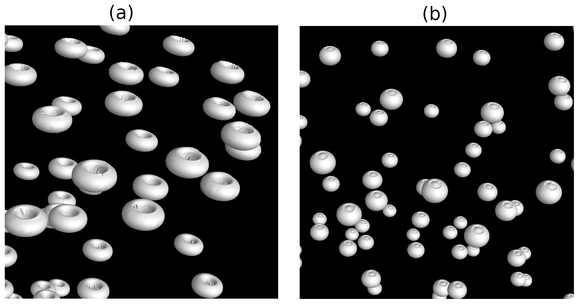
Figure 53D views of the determined surfaces of the reconstructed volume data from the simulations with all static misalignments with initially estimated magnitudes (a) and 20 % of those initially estimated magnitudes (b). The views show that a CT system this heavily misaligned will not be considered for system verification as it is visually not producing correct measurements. Even with 20 % misalignment, the spheres have a visible deformation from the spherical form.
Therefore, we decided to reduce the magnitude of the static geometry misalignments by simulating only one misalignment at a time and inspecting the measurement errors produced. We claim that a reasonable dimensional CT system should produce errors in the sphere centre-to-centre measurements within 10–20 µm (better values are possible but defy the purpose of this study). Therefore, we decreased the magnitude of all static geometry errors iteratively from 100 % to 50 % and continued halving the magnitude until the single misalignment inspected produced maximum SD errors within the desired range of 10–20 µm. The single misalignments were always simulated with a positive and a negative sign (i.e., e.g. for a rotation axis tilt of 0.2∘, both a simulation with the axis tilted by 0.2∘ and one with the axis tilted by −0.2∘ were conducted).
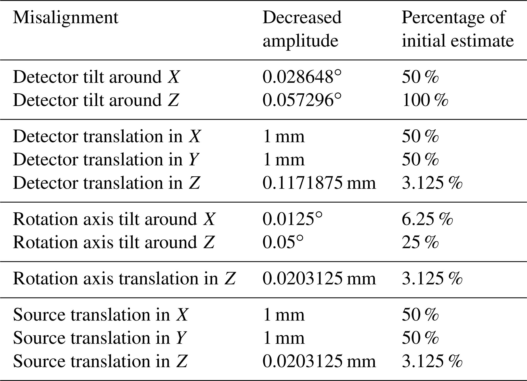
The resulting misalignment amplitudes are shown in Table 2. The misalignments that were most in need of amplitude reduction were all translations in the z direction (scaling errors) and the rotation axis tilt around the x axis. We want to model a realistic CT system in this work. It thus makes sense to assume that misalignments that are adjusted and calibrated the same way during system setup should not have different maximum misalignments. Consequently, we grouped all detector tilts to an amplitude of 0.028648∘ and all rotation axis tilts to an amplitude of 0.0125∘. The reader might notice the absence of the tilts around the y axis in the table. This is due to the fact that the detector tilt around the y axis did not result in any discernible increase of SD errors, while the rotation axis is aligned with the y axis, and its tilt around the y axis only changes its direction combined with further tilts around the other axes.
As discussed in Sect. 2, the linearity of the SD errors (indicated by a correlation coefficient) or the linearity of the maximum SD errors with the nominal distance is of interest. For the misalignments producing scaling errors (detector, source and rotation axis translation in beam direction), we obtained the expected result that ρ≈1. These misalignments, which in our experience are the dominant error sources in real CT systems, are therefore completely unproblematic in the context of our study. To suppress the influence of these dominant geometrical misalignments to the desired value of 10–20 µm maximum SD errors, we had to scale them down to 3.125 % of the initial estimate. The rotation axis tilt around the x axis (axis perpendicular to beam and rotation axis) has a correlation coefficient of ρ≈0.9; all other misalignments have a correlation coefficient below 0.6. All misalignments but the scaling sources thus show more complex behaviour that merits a closer analysis, which is presented in Sect. 5.
Table 2Overview of decreased amplitudes of static geometrical misalignments to yield maximum SD errors within 10–20 µm. For a comment on the omission of the detector tilt around Y and the rotation axis tilt around Y, see the explanation in Sect. 4.1.
4.2 Dynamic geometric misalignments
Real rotary tables do not exhibit just one single dynamic deviation from the ideal rotation but do rather always show a combination of different dynamic misalignments. Therefore, we simulated the combination of these misalignments. As described in Sect. 3.1, the Fourier series approach has 11 degrees of freedom in the 11 phase angles Φk that need to be chosen. We generated 50 sets of 11 pseudo-random phase angles in the interval [0,2π] (uniform distribution) with MATLAB R2021a and simulated 50 CT scans with the resulting dynamic misalignments modulated according to Eq. (2). Our initial hypothesis was that the resulting measurement errors would have a mean value and that the influence of the phase angles would be a small perturbation. This is however not the case (compare Fig. 6). The values of the phase angles have a deciding influence on the SD errors measured. For no set of phase angles is there a linearity of the SD errors with respect to the nominal distance (for all phase angles, the correlation coefficient is below 0.5). Therefore, a more in-depth analysis is necessary in Sect. 5.

Figure 6Histograms of the ratio between standard deviation σ and average value <m> of the measurement deviation in the sphere centre-to-centre distances. The standard deviation and average are calculated per sphere pair over all 50 different phase angle sets (compare Sect. 4.2). For these histograms, the signed values of the measurement deviations are used. The left histogram (a) shows the range between the 1st and the 99th percentile, and the right histogram (b) shows the centre in detail. The histograms show that the different phase angles have a substantial impact on the measurement deviation and that there is no meaningful “average deviation” for all phase angles (from which the selection of a specific set of phase angles would only induce a small perturbation).
Based on this result, we needed to select a specific representative set of phase angles for further simulations combining dynamic and static misalignments (Sect. 4.3). A simulation of all 50 phase angles requires multiple days of computation time – therefore, simulating more phase angles or performing combined simulations with different phase angles would not have been feasible due to the necessary computation times. Our intention in selecting a specific set of phase angles was that it should be an “average” case, containing, at all nominal measurement lengths, a wide and homogeneous distribution of low and high SD errors.
Practically, we devised the following selection procedure:
-
For each sphere distance, the maximum value of the measurement error over all 50 phase angle set simulations was calculated.
-
All measurement errors were converted into percentages of their respective maximum value from the first step.
-
A bivariate histogram of percentual measurement errors from the second step and their respective nominal sphere distance was calculated for each phase angle set.
-
To account for the different number of measurement distances in different nominal distance bins of the histogram (compare Fig. 3), the histogram values were normalised by their total counts in each nominal sphere distance bin (i.e., the number of nominal distances in this bin). This means that each histogram entry now stands for the ratio of nominal distances in this nominal distance bin width that produced an SD error within this SD error bin. The more homogeneous this number is across the bins, the more homogeneous the distribution is. An example for the resulting histogram is shown in Fig. 7.
-
In each nominal distance bin, the standard deviation of the ratios in the different SD error bins was calculated. Then, the arithmetic mean value of all these standard deviations was calculated.
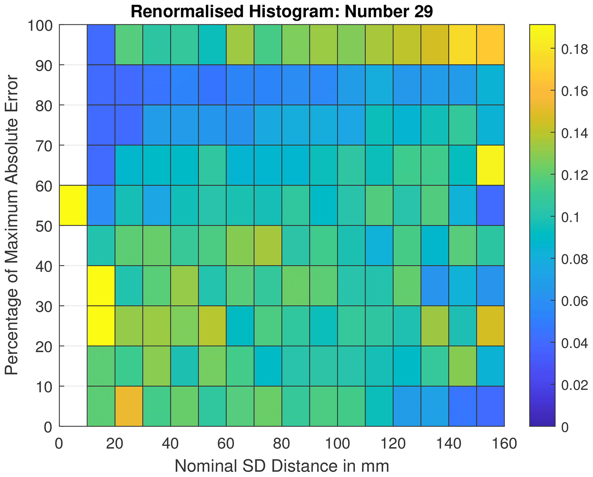
Figure 7Renormalised bivariate histogram of SD measurement errors and nominal sphere distances as explained in Sect. 4.2. The phase angle set number 29 is the one with the lowest value of (meaning that the error distribution is most wide and most homogeneous) and thus the one selected for further simulations.
The phase angle simulation with the lowest value of is the simulation that produces the most homogeneous and wide distribution of SD errors across all nominal distances. Thus, it is the most relevant phase angle set for this investigation and was used furthermore for the subsequent simulations.
The simulation with dynamic misalignments using the selected phase angles and the initial misalignment amplitudes estimated in Sect. 3.1 has a maximum SD error of above 100 µm. As in Sect. 4.1, we again wanted to decrease misalignment amplitudes such as to reach a maximum SD error between 10–20 µm. Therefore, we reduced all dynamic misalignment amplitudes in steps of 10 % of their initial value. At 20 % of the initial value, a maximum SD error of 18.3 µm was reached. We repeated the simulations with negative misalignment amplitudes and obtained approximately the same result (maximum SD error of 18.8 µm at 20 %).
4.3 Simulations with combined misalignments
We performed two sets of simulations with all static and all dynamic misalignments (with the phase angle set selected in Sect. 4.2) combined. In the first set of simulations (IV from Table 1), we used the misalignment amplitudes that we had initially estimated (in Sect. 3.1). We think that these simulations represent a CT system which has quickly been aligned and is “low-effort”. As a second set of simulations (V from Table 1), for each misalignment, the chosen amplitudes that produce errors within 10–20 µm were used. This set of parameters represents a CT system in which dominant geometrical error sources have been characterised and mitigated. Therefore, it represents a “medium-effort” CT system.
For both parameter sets, the initial misalignment amplitudes in their combination produced unrealistically high SD errors (or, in the case of set IV, simulations resulting in volumes as seen in Fig. 5). Consequently, all misalignment amplitudes were reduced by multiplication with a common factor. For the low-effort CT system set IV, the factors ±0.2, ±0.15, …, ±0.05 were simulated. For the medium-effort CT system set V, the factors ±1, ±0.8, …, ±0.2 were simulated.
In all simulations with combined misalignments, there is no linearity of the SD errors with respect to the nominal sphere distance. For set IV, all correlation coefficients are below 0.8. For set V, all correlation coefficients are below 0.5. The difference is noticeable and might be due to the dominating scaling errors in the set IV.
Therefore, it is not possible to conclude that these simulations are not relevant to the question of suitable measurement lengths for MPE determination. However, as discussed in Sect. 2, this does not allow for any conclusion about these simulations. For both sets, a further analysis of the behaviour was necessary and will be described in Sect. 5.
In Sect. 5.1, the automated identification method for non-linear cases that might necessitate a measurement above 66 % is presented. Subsequently, in Sect. 5.2, the results from applying this method to the simulations are outlined.
5.1 Automated detection method
In acceptance and reverification testing, calibrated sphere centre-to-centre distances are measured (compare E DIN EN ISO 10360-11:2021-04, 2021; VDI/VDE 2630 Blatt 1.3, 2011). The error in measuring these distances needs to be below the manufacturer-specified maximum permissible error (MPE). MPEs should be specified as a constant value, a linear function of the nominal measurement distance or a linear function limited by a constant value (definition 9.2 of ISO 10360-1 (DIN EN ISO 10360-1:2003-07, 2003)). In the VDI/VDE standard (VDI/VDE 2630 Blatt 1.3, 2011), the ISO 10360-2 standard on tactile coordinate measuring machines (DIN EN ISO 10360-2:2010-06, 2010, Sect. 6.3.2), the ISO 10360-7 standard on coordinate measuring machines with imaging probing systems (DIN EN ISO 10360-7:2011-09, 2011, Sect. 6.2.2) and the ISO 10360-8 standard for coordinate measuring machines with optical distance sensors (DIN EN ISO 10360-8:2014-03, 2014, Sect. 6.3.2) as well as the ASME standard on CTs (ASME B89.4.23-2020, 2020, Sect. 7.4.1), distances of up to 66 % of the maximum measurement distance of the coordinate measuring machine have to be measured for an acceptance or reverification test. The current draft of the ISO 10360-11 (E DIN EN ISO 10360-11:2021-04, 2021) requires measurements of sphere distances of up to 85 %. This requirement makes sense if there are effects between 66 % and 85 % of the maximum measurement distance that necessitate a different MPE specification than below. In light of the form of the MPE specification, these effects would need to be non-linear in the measurement length. The MPE specification should follow the form given by Eq. (3).
Here, the manufacturer can choose A and K freely. The extreme choices are obviously A=0 (minimising K) or K→∞ (maximising A). Any effect necessitating measurements of up to 85 % would therefore mean that the manufacturer would need to change their choice of A and K because of the additional data above 66 %. The choice of the values for A and K is (and ought to be) at the discretion of the manufacturer – therefore, no clear criterion can be derived from the standard. We however propose to inspect the convex hull (see O'Rourke, 1998) of the point set of nominal measurement distances and respective measurement deviations. If the convex hull below 66 % stays constant no matter whether all points or only the points up to 66 % are used, there is no reason for a requirement to measure lengths longer than 66 %, and this simulated case is deemed not relevant for the MPE question. If however, the convex hull does change, this simulated case should be inspected as it might be relevant. The approach is illustrated in Figs. 8 and 9.
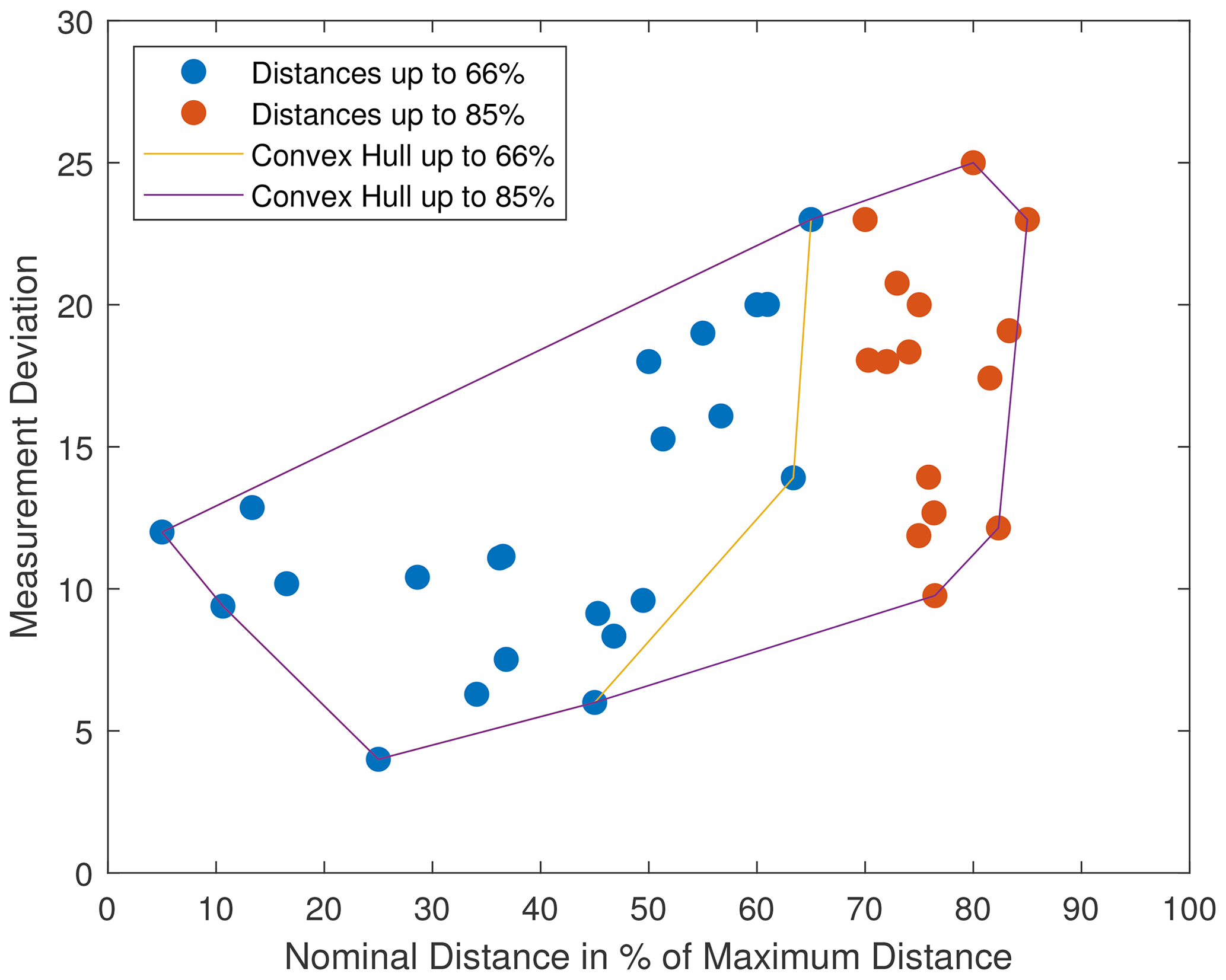
Figure 8A scenario in which the convex hulls of the measurement points below 66 % and of all measurement points (including above 66 %) agree up until 66 %. We assume that an MPE specification according to Eq. (3) based on the points below 66 % would encompass the points above 66 % as well.
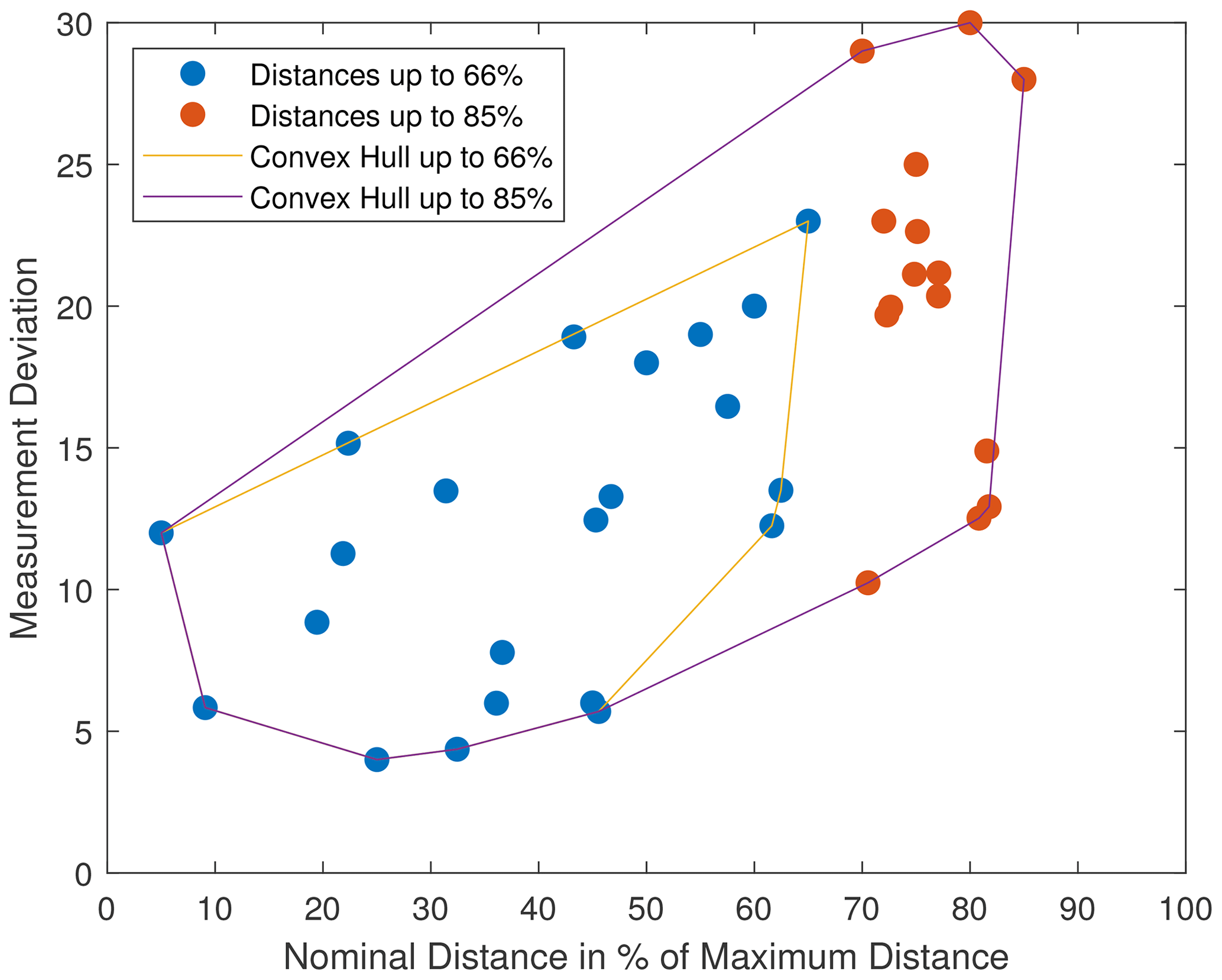
Figure 9A scenario in which the convex hulls of the measurement points below 66 % and of all measurement points (including above 66 %) do not agree below 66 %. There are points above 66 % whose increase in measurement deviation is stronger than linear, and thus we think that in this case, an MPE specification for both point sets (up until 66 % and all points) could reasonably be different. A MPE specification for below 66 % might not hold for the points above. Such an extreme scenario as depicted here could not be observed in any simulation of this study.
In contrast to Figs. 8 and 9, we truncate the bottom part of the convex hull, using only parts with positive slope. Further, we do not consider any decreases in the slope of the 66 % convex hull that happen in the regime between 60 % and 66 % as relevant as these can be boundary effects, and we do not believe a manufacturer would readjust their MPE specification based on these.
The convex hull criterion as presented here is a worst-case scenario as there is no safety distance to the measured points, and the last (and therefore lowest) slope of the 66 % convex hull is used for comparison. The choice of a higher slope is legitimate and is an added safety margin for the manufacturer. Further, accounting for the test value uncertainty, any manufacturer will keep a certain distance to all measurement points when constructing an MPE. We therefore think that in a real MPE specification scenario, the MPE will be chosen with more of a safety margin. The convex hull criterion does however allow for the automatic identification of cases which are definitely not relevant for the question of maximum length (i.e., those for which the convex hulls agree). The cases in which the convex hulls do not agree need visual inspection – the criterion does not allow for an automated decision that, based on this data set, a measurement of lengths longer than 66 % is necessary. This is again due to the flexibility in the MPE statement and the resulting need for a visual inspection.
To quantify the difference between both convex hulls (if there is any), we extend the last clockwise part of the convex hull with a positive slope into a linear function (representing a “convex-hull-derived” MPE specification). If both convex hulls differ below 66 % (as in the Fig. 9), there needs to be at least one data point above the extended linear function derived from the 66 % convex hull. To quantify the difference, we use the maximum distance of all these data points from this extended linear function. The distance is measured in the direction of the “measurement deviation” axis only. Returning to the argument of a reasonable MPE specification by a manufacturer, we quantify this distance as a percentage of the observed measurement deviation at this data point. The motivation is that a manufacturer will choose a safety distance; thus exceeding this worst-case MPE statement by a few percent is not relevant.
5.2 Results
Out of a total of 164 simulations from Sect. 4.1 and 4.2 (single static misalignments and isolated dynamic misalignments), only seven show a maximum difference that is more than 5 % of the measured SD error. Two of these are tilts of the rotation axis around the x axis (axis perpendicular to beam and rotation axis; see Fig. 2) by −0.0125 and −0.025∘ (see Fig. 10). The data points in those plots follow a roughly linear trend, and, thus, we expect a human to specify a MPE following this general linear trend. The other five are dynamic simulations with random phase angles from Sect. 4.2 (see Fig. 11 and the first plot of Fig. 12).

Figure 10Convex hull analysis of non-linearity for the rotation axis tilt around the x axis (axis perpendicular to beam and rotation axis; see Fig. 2) by −0.0125 and −0.025∘. The plots show the data points, both convex hulls (using points until 66 % and using all points) as well as derived MPE specifications. The Δabs marks the data point with the largest distance to the 66 % MPE specification. The simulations are part of simulation set I. We are convinced that a human would visually not specify such a low slope for the below 66 % MPE specification as the automated algorithm used in this study. In this sense, the criterion employed here is, as discussed in the text, a worst-case criterion. We would expect most MPEs specified based on this picture to follow the general linear trend of the data points.
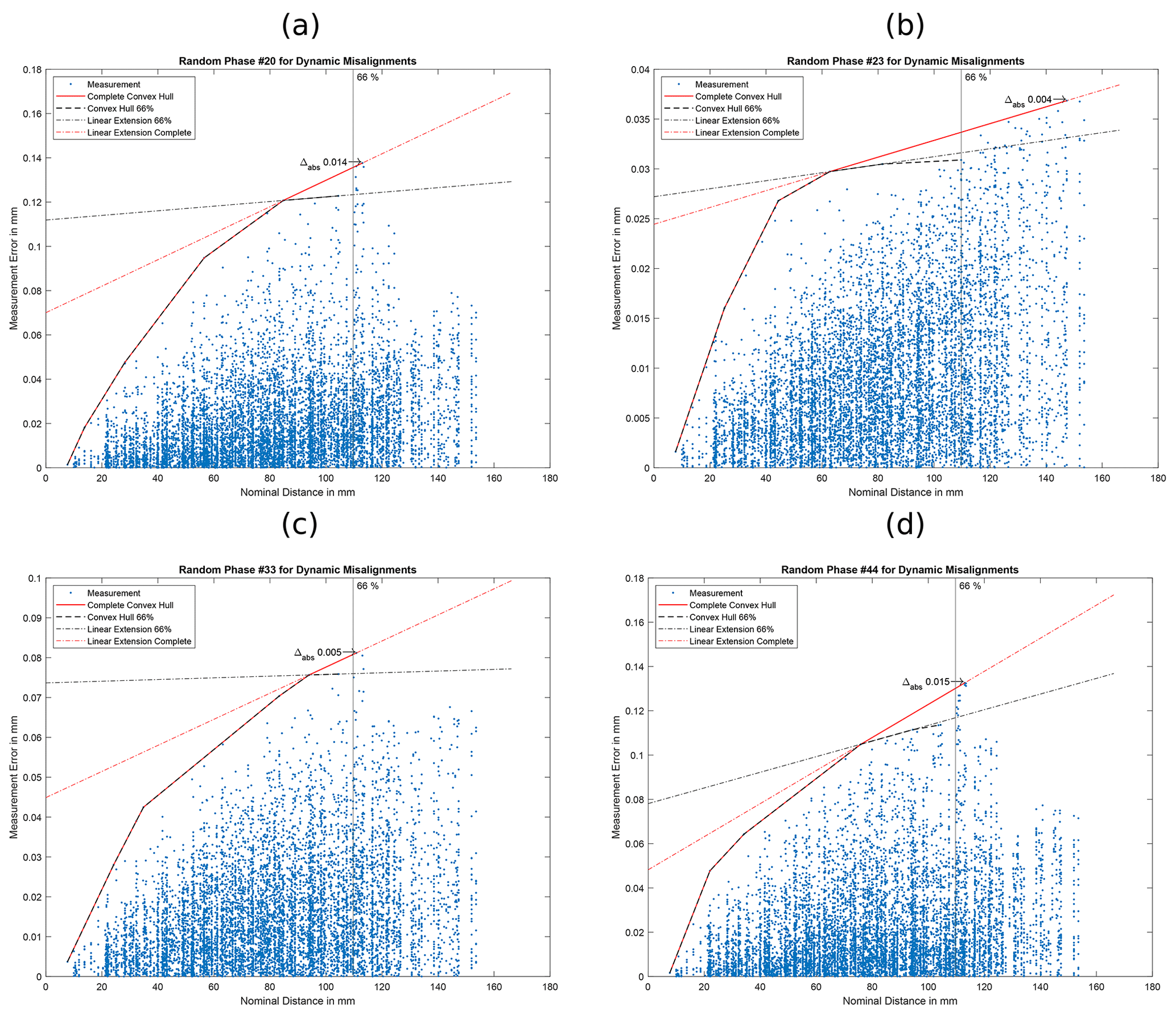
Figure 11Convex hull analysis of non-linearity: the plots show the data points, both convex hulls (using points until 66 % and using all points) as well as derived MPE specifications. The Δabs marks the data point with the largest distance to the 66 % MPE specification. The plots are for four of the five simulations with random phase angles from Sect. 4.3 and part of simulation set II (for the last one, see Fig. 12).
For the simulations with the combined errors (Sect. 4.3), we performed the same analysis. For the initial misalignment estimate simulations (set IV, eight simulations), no simulation shows a difference above 5 %. For the simulations with adapted misalignment amplitudes (set V, 10 simulations), three simulations show a difference above 5 % (see Fig. 12). This finding agrees with the increase in correlation coefficient ρ (compare Sect. 4.3) and the hypothesis of dominating scaling errors for set IV as scaling errors are strictly linear in the measurement length.
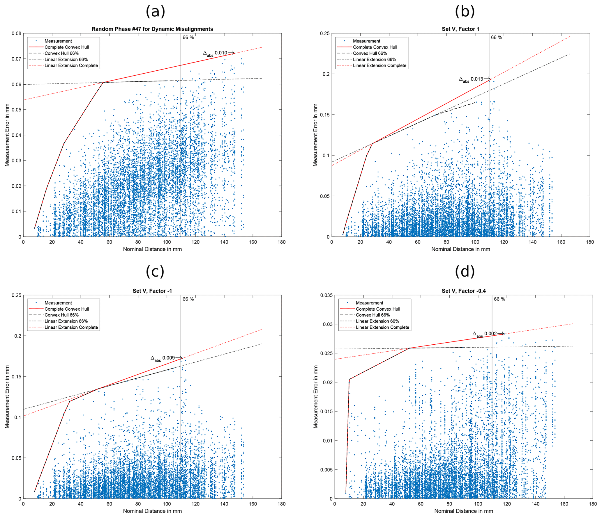
Figure 12Convex hull analysis of non-linearity: the plots show the data points, both convex hulls (using points until 66 % and using all points) as well as derived MPE specifications. The Δabs marks the data point with the largest distance to the 66 % MPE specification. The plot (a) is the last one for the simulations for the five random phase angles from Sect. 4.3 and part of simulation set II (for the first four, see Fig. 11). The other three plots (b), (c) and (d) are for simulation set V (see Sect. 4.3).
Summarising, from 182 simulations, only 10 are identified as possibly relevant by the convex hull criterion due to a difference of more than 5 % between both convex hulls. As discussed above, this does not necessarily mean that they would actually fail a manufacturer's MPE specification above 66 % due to the freedom in specifying the MPE. Of these 10 cases, two (the rotation axis displacement) have a general linear trend that would probably lead to an MPE with a higher slope in specification (these can visually be classified as “roughly linear” in the sense of Fig. 1). The other eight cases are five sets of random phase angles for the dynamic errors (Figs. 11 and 12) and three simulations with combined misalignments with rescaled amplitudes (set V; see Fig. 12). These cases will be discussed again in Sect. 6.
As described in Sect. 3.3, probing form errors were also evaluated. Besides sphere distances, probing form errors are another important characteristic in acceptance testing (E DIN EN ISO 10360-11:2021-04, 2021; VDI/VDE 2630 Blatt 1.3, 2011). A complete specification is required to cover at least probing errors (probing form errors and probing size errors) and the sphere distance errors (Table 3 in E DIN EN ISO 10360-11:2021-04, 2021). Therefore, these characteristics should be seen as a set of indicators about CT system performance. It is not necessary that all characteristics detect all possible error sources. We therefore analyse the impact of the geometrical misalignments simulated thus far on the probing form errors. The rationale behind this is that the eight cases needing a visual – and thus necessarily subjective – analysis in Sect. 5 do not need to be analysed further if the probing form error is very sensitive to them. In the latter case, the probing form error will detect the underlying geometrical misalignment sufficiently, and therefore, even if the misalignments are not completely accounted for in the MPE statement (“not completely accounted for” should be read as “underestimated by a few percent”), there is no risk that the misalignment is not detected during acceptance or reverification testing.
Within this section, we analyse the sphere-wise increase in form error in a simulation with misalignment in comparison to a simulation without misalignment. Further, we report the maximum increase in form error over all spheres.
For the 50 random phase angle simulations with the dynamic misalignments (set II), the probing form error increase is above 100 µm for all phases and above 200 µm for most. We claim that these values will not be acceptable to a customer and that therefore, the potential that – for 10 % of these simulations – the MPE specification for sphere distance errors might be too low based on data points up to 66 % (compare Figs. 11 and 12) is not crucial as another part of the acceptance test will more reliably detect the underlying misalignment.
For the set of combined misalignments based on the rescaled simulations (set V), all probing form error increases are above 270 µm. Therefore, the misalignments can well be detected using the probing form error test, and the potential that, for some of these simulations, the MPE specification for the sphere distance errors might be too low based on the data up to 66 % (compare Fig. 12) can again be neglected as the probing form error part of the acceptance test will easily detect the geometrical misalignments.
For the set of combined initial estimate misalignments (set IV), the probing form errors are above 300 µm for factors with magnitude greater or equal to 0.1. For the factor ±0.05, the probing form errors are at approximately 32 µm. This is still a noticeable probing form error, but it is much more realistic. With set IV, we did not identify any potentially relevant cases in Sect. 5. This simulation shows that different parts of the acceptance test are sensitive to different misalignments. Both the lowest factors of set IV and set V lead to comparable SD errors, but their probing form error differs by an order of magnitude. The scaling errors that are dominant in set IV thus seem to have a much lower impact on the probing form errors (see discussion below).
The static geometry misalignments (simulation set I) merit a more in-depth discussion:
-
Detector position perpendicular to beam axis (x and y axis). For the detector translations perpendicular to the beam axis, probing form errors are very high (all above 100 µm). Probing form errors seem very sensitive to this misalignment.
-
Detector position along beam axis (z axis). Only for a high misalignment of 3.75 mm or −3.75 mm are the probing form errors above 10 µm (10.5 µm or 15.2 µm). For all smaller misalignments, the probing form errors are below 8 µm. The probing form errors are therefore not very suitable to detect this misalignment that causes strong scaling errors.
-
Detector orientation. For the detector tilt around the x and y axis, the probing form errors are below 5 µm – probing form errors are not very sensitive to these misalignments. For the tilt around the z axis, the probing form errors are higher and reach approximately 17 µm for a 0.057296∘ tilt.
-
Source position. For the translation along the x axis, the probing form errors are high (all above 340 µm). Along the y axis, the probing form errors are considerably smaller, with approx. 18 µm at the setting producing SD errors within 10–20 µm. The scaling error (z axis translation) induces small probing form errors below 9 µm. For the z axis translation of the source that leads to SD errors within 10–20 µm, the probing form errors are below 2 µm. Therefore, also for this scaling error, probing form errors are again not very suitable for detecting the geometrical misalignment.
-
Rotation axis tilt. A rotation axis tilt around the z axis by ±0.05∘ (leading to SD errors within 10–20 µm) produces probing form errors of 17 µm or 18 µm. The rotation axis tilt around the x axis results in small probing form errors below 7 µm for absolute misalignment amplitudes of ± 0.025∘ and below. Unlike with scaling errors, the increase of probing form errors with increasing misalignment amplitude is stronger (15 µm or 14 µm at ± 0.05∘ and 31 µm at ±0.1∘), but the amplitude that results in SD errors within 10–20 µm does not result in equally high or higher probing form errors.
-
Rotation axis position. For translations along the beam direction (z axis), probing form errors are below 8 µm. At the magnitude that leads to SD errors within 10–20 µm, the form errors are below 2 µm. Again, the scaling error does not impact form errors strongly.
Summarising, dynamic misalignments of the rotation axis and the rotary table can be detected very well by inspecting probing form errors, while scaling misalignments lead to negligible probing form errors. Other static misalignments show a more complex dependence – with some resulting in large probing form errors, while others have less of an impact. The simulation study clearly shows the need for including both probing form errors and sphere distance measurements in acceptance testing as both are sensitive to different geometrical misalignments.
The eight cases mentioned at the end of Sect. 5.2 as cases in which the data points for SD errors above 66 % might necessitate a different choice for the MPE are all cases in which probing form errors are very pronounced and furthermore cases in which misalignments that are very well captured by probing form errors cause the SD errors. We therefore think that these cases are negligible for acceptance testing seen as a whole, as the probing form error will detect the underlying misalignments reliably, and that these eight cases are thus no reason for a requirement to measure lengths above 66 % for the SD errors.
We performed a simulative study to investigate sphere distance and form measurements that are typically used in acceptance and reverification testing (see, for example, E DIN EN ISO 10360-11:2021-04, 2021; VDI/VDE 2630 Blatt 1.3, 2011). For this purpose, we designed a virtual simulation artefact and estimated several geometrical misalignments. Our initial estimates of the geometrical misalignments mostly produced unrealistically high measurement errors for the sphere distances. We therefore needed to reduce our initial estimates. We discussed the problem of finding a suitable automated identification for whether a simulation would indicate a need for deviating from the established 66 % measurement rule for sphere distances (as included in DIN EN ISO 10360-2:2010-06, 2010; DIN EN ISO 10360-7:2011-09, 2011; DIN EN ISO 10360-8:2014-03, 2014; VDI/VDE 2630 Blatt 1.3, 2011). We presented a worst-case criterion based on constructing the convex hull of the data points collected and used this to evaluate our simulations. Of a total of 182 simulations, only 10 were identified based on this worst-case criterion. Two of these were gauged as having a linear trend and thus being a shortcoming of the criterion. The other eight are due to simulations with dynamic rotary table misalignments. In general, the test procedure in acceptance and reverification testing should characterise CT system performance and thus also detect any geometrical misalignments. It is therefore important that at least one of the mandatory characteristics (probing error (form or size) or sphere distance error) of the standardised test is able to detect each geometrical misalignment. It is however not necessary that each characteristic does so or that each characteristic does so with a high sensitivity. We therefore also inspected the impact of geometrical misalignments on the probing form errors. This analysis showed that the misalignments that produce the smallest probing form errors are the scaling misalignments that produce sphere distance errors linear in the nominal measurement distance. All other misalignments can – to some extent – be detected by probing form errors as well.
Even for most geometrical misalignments that are well detected by probing form errors, there is, according to our worst-case convex hull criterion, no behaviour that would necessitate a deviation from the established 66 % requirement. The dynamic rotary table misalignments result in especially pronounced probing form errors. In the eight cases in which dynamic rotary table misalignments are present and the convex hull criterion indicates a possibility for a need to measure longer lengths, the underlying misalignments can therefore be well identified by inspecting the probing form error. An extension of the measurement lengths for the SD error to capture these misalignments even better with the SD error as well would constitute unnecessary additional effort as the probing form error is clearly more sensitive.
Overall, the highest deviations from the conservative MPE estimate derived based on the convex hull are 8 % of the measured SD error – we think that considering test value uncertainty, manufacturer safety margin and freedom of choice in the MPE specification, the MPE specification will rarely be below this error. Should it happen, both user and manufacturer still have a clear indication for the underlying geometrical misalignment from high probing form errors. Besides the roughly linear behaviour of the rotation axis tilt around the x axis which was found by our automated convex hull criterion but which we visually discarded, there is no scenario in which, due to more than linear behaviour, a geometrical misalignment can not be detected neither with the SD measurements up to 66 %, nor with the form measurements. As both are mandatory, no user or manufacturer can perform an acceptance test without detecting the geometrical misalignments studied in this work.
Based on the simulation study presented here, there is no technical reason for measuring SD errors with nominal lengths above the established 66 % of the maximum length from other comparable standards (DIN EN ISO 10360-2:2010-06, 2010; DIN EN ISO 10360-7:2011-09, 2011; DIN EN ISO 10360-8:2014-03, 2014; VDI/VDE 2630 Blatt 1.3, 2011).
The code is not publicly accessible but can be requested from the corresponding author if required.
Due to the size (more than 6 TB), the simulation data are not publicly available and can be requested from the authors if needed.
The author contributions are declared according to CASRAI CRediT. KDI, WK, IS, TH and FW were involved in conceptualisation and methodology. FW was responsible for data curation, formal analysis, investigation, project administration, software, visualisation and writing – original draft. KDI, WK, IS and TH were responsible for supervision and writing – review and editing.
Werth Messtechnik GmbH and Carl Zeiss Industrielle Messtechnik GmbH are manufacturers of industrial computed tomography systems. This study received funding from these companies.
Publisher’s note: Copernicus Publications remains neutral with regard to jurisdictional claims in published maps and institutional affiliations.
We want to thank Werth Messtechnik GmbH and Carl Zeiss Industrielle Messtechnik GmbH for the financial support of the project as well as Volume Graphics GmbH (Heidelberg, Germany) for the kind permission to use their VGSTUDIO MAX evaluation software.
This study received funding from Werth Messtechnik GmbH and Carl Zeiss Industrielle Messtechnik GmbH.
This paper was edited by Thomas Fröhlich and reviewed by two anonymous referees.
ASME B89.4.23-2020: X-Ray Computed Tomography (CT) Performance Evaluation, ISBN 9780791873830, 2020. a, b, c, d, e
Bellon, C., Deresch, A., Gollwitzer, C., and Jaenisch, G.-R.: Radiographic Simulator aRTist: Version 2, in: 18th World Conference on Nondestructive Testing, 16–20 April 2012, Durban, South Africa, http://www.ndt.net/?id=12664 (last access: 10 June 2022), 2012. a, b
Carmignato, S., Dewulf, W., and Leach, R. (Eds.): Industrial X-Ray Computed Tomography, 1st edn., Springer International Publishing, ISBN 978-3-319-59573-3, https://doi.org/10.1007/978-3-319-59573-3, 2018. a
DIN EN ISO 10360-1:2003-07: Annahmeprüfung und Bestätigungsprüfung für Koordinatenmessgeräte (KMG) Teil 1: Begriffe (enthält Berichtigung AC:2002) (ISO 10360-1:2000 + Cor.1:2002), 2003. a, b, c
DIN EN ISO 10360-2:2010-06: Geometrische Produktspezifikation (GPS) – Annahmeprüfung und Bestätigungsprüfung für Koordinatenmessgeräte (KMG) – Teil 2: KMG angewendet für Längenmessungen (ISO 10360-2:2009), 2010. a, b, c
DIN EN ISO 10360-3:2000-08: Geometrische Produktspezifikation (GPS) Annahmeprüfung und Bestätigungsprüfung für Koordinatenmessgeräte (KMG) Teil 3: KMG mit der Achse eines Drehtisches als vierte Achse (ISO 10360-3:2000), 2000. a
DIN EN ISO 10360-7:2011-09: Geometrische Produktspezifikation (GPS) – Annahme- und Bestätigungsprüfung für Koordinatenmessgeräte (KMG) – Teil 7: KMG mit Bildverarbeitungssystemen (ISO 10360-7:2011), 2011. a, b, c
DIN EN ISO 10360-8:2014-03: Geometrische Produktspezifikation und -prüfung (GPS) – Annahme- und Bestätigungsprüfung für Koordinatenmesssysteme (KMS) – Teil 8: KMG mit optischen Abstandssensoren (ISO 10360-8:2013), 2014. a, b, c
E DIN EN ISO 10360-11:2021-04: Geometrische Produktspezifikation und -prüfung (GPS) – Annahmeprüfung und Bestätigungsprüfung für Koordinatenmessgeräte (KMG) – Teil 11: Computertomografie (ISO/DIS 10360-11:2021), 2021. a, b, c, d, e, f, g, h, i, j
Fahrmeir, L., Kneib, T., and Lang, S.: Regression, 2nd edn., Springer Berlin Heidelberg, ISBN 978-3-642-01837-4, https://doi.org/10.1007/978-3-642-01837-4, 2009. a
Jaganmohan, P., Muralikrishnan, B., Shilling, M., and Morse, E. P.: Trends in Geometric Error of X-ray Computed Tomography Instruments Observed at Different Locations in the Measurement Volume, in: ASPE 2020 Annual Meeting Volume 73, 122–127, ISBN 978-1-7138-2046-8, 2020. a, b, c, d, e
Muralikrishnan, B., Shilling, M., Phillips, S., Ren, W., Lee, V., and Kim, F.: X-ray Computed Tomography Instrument Performance Evaluation, Part I: Sensitivity to Detector Geometry Errors, J. Res. Natl. Inst. Stan., 124, 124014, https://doi.org/10.6028/jres.124.014, 2019a. a, b, c, d, e, f, g, h
Muralikrishnan, B., Shilling, M., Phillips, S., Ren, W., Lee, V., and Kim, F.: X-ray Computed Tomography Instrument Performance Evaluation, Part II: Sensitivity to Rotation Stage Errors, J. Res. Natl. Inst. Stan., 124, 124015, https://doi.org/10.6028/jres.124.015, 2019b. a, b, c, d, e, f, g
Muralikrishnan, B., Shilling, M., Phillips, S., Ren, W., Lee, V., Kim, F., Alberts, G., and Aloisi, V.: X-ray computed tomography instrument performance evaluation: Detecting geometry errors using a calibrated artifact, in: Dimensional Optical Metrology and Inspection for Practical Applications VIII, edited by: Zhang, S. and Harding, K. G., SPIE, https://doi.org/10.1117/12.2518108, 2019c. a, b, c, d, e
O'Rourke, J.: Computational Geometry in C, 2nd edn., Cambridge University Press, ISBN 9780511804120, https://doi.org/10.1017/cbo9780511804120, 1998. a
van Aarle, W., Palenstijn, W. J., Beenhouwer, J. D., Altantzis, T., Bals, S., Batenburg, K. J., and Sijbers, J.: The ASTRA Toolbox: A platform for advanced algorithm development in electron tomography, Ultramicroscopy, 157, 35–47, https://doi.org/10.1016/j.ultramic.2015.05.002, 2015. a
van Aarle, W., Palenstijn, W. J., Cant, J., Janssens, E., Bleichrodt, F., Dabravolski, A., Beenhouwer, J. D., Batenburg, K. J., and Sijbers, J.: Fast and flexible X-ray tomography using the ASTRA toolbox, Opt. Express, 24, 25129–25147, https://doi.org/10.1364/oe.24.025129, 2016. a
VDI/VDE 2617 Blatt 4: Leitfaden zur Anwendung von DIN EN ISO 10360-3 für Koordinatenmessgeräte mit zusätzlichen Drehachsen, May 2006. a
VDI/VDE 2630 Blatt 1.3: Leitfaden zur Anwendung von DIN EN ISO 10360 für Koordinatenmessgeräte mit CT-Sensoren, December 2011. a, b, c, d, e, f, g, h, i, j, k
Wohlgemuth, F., Müller, A., and Hausotte, T.: Development of a virtual metrological CT for numerical measurement uncertainty determination using aRTist 2, tm – Technisches Messen, 85, 728–737, https://doi.org/10.1515/teme-2018-0044, 2018. a
Wohlgemuth, F., Wolter, F., and Hausotte, T.: Digitale Zwillinge metrologischer Röntgencomputertomografen für die numerische Messunsicherheitsbestimmung, in: ZfP heute. Wissenschaftliche Beiträge zur zerstörungsfreien Prüfung 2020, edited by: Deutsche Gesellschaft für Zerstörungsfreie Prüfung e.V., pp. 106–110, ISBN 978-3-947971-10-7, https://www.ndt.net/?id=25501 (last access: 10 June 2022), 2020. a
- Abstract
- Introduction
- Linearity and MPE-relevant behaviour
- Simulative setup
- Simulated misalignment scenarios
- (Non-)Linearity
- Probing form errors
- Conclusions
- Code availability
- Data availability
- Author contributions
- Competing interests
- Disclaimer
- Acknowledgements
- Financial support
- Review statement
- References