the Creative Commons Attribution 4.0 License.
the Creative Commons Attribution 4.0 License.
 | 25 Apr 2023
Approximate sequential Bayesian filtering to estimate 222Rn emanation from 226Ra sources using spectral time series
Stefan Röttger
Annette Röttger
A new approach to assess the emanation of 222Rn from 226Ra sources based on γ-ray spectrometric measurements is presented. While previous methods have resorted to steady-state treatment of the system, the method presented incorporates well-known radioactive decay kinetics into the inference procedure through the formulation of a theoretically motivated system model. The validity of the 222Rn emanation estimate is thereby extended to regimes of changing source behavior, potentially enabling the development of source surveillance systems in the future. The inference algorithms are based on approximate recursive Bayesian estimation in a switching linear dynamical system, allowing regimes of changing emanation to be identified from the spectral time series while providing reasonable filtering and smoothing performance in steady-state regimes. The derived method is applied to an empirical γ-ray spectrometric time series obtained over 85 d and is able to provide a time series of emanation estimates consistent with the physics of the emanation process.
- Article
(3463 KB) - Full-text XML
- BibTeX
- EndNote


222Rn is an odorless, colorless, radioactive noble gas, occurring naturally in the environment as part of the primordial 238U decay chain. Due to its high mobility in the environment, radon can accumulate inside buildings where, in conjunction with its decay products (short-lived progeny; SLP), it is responsible for the most significant natural exposure of the general public to ionizing radiation, which is an important consideration for incidents of lung cancer (Darby et al., 2005). In the 2013/59/EURATOM treaty, 300 Bq m−3 was stipulated as the action level for indoor 222Rn activity concentrations, beyond which mitigation is required. On the other hand, however, measurements of outdoor 222Rn activity concentration at environmental levels have numerous beneficial applications in environmental sciences, including (but not limited to): as a tracer of terrestrial influence on air masses (Chambers et al., 2016, 2018); as a tool for classifying the atmospheric mixing state (e.g., Perrino et al., 2001; Williams et al., 2013, 2016; Chambers et al., 2019b, a); and as a tool for estimating integrated local- to regional-scale emissions of trace gases with similarly distributed sources, such as CH4, N2O, or CO2 (Levin, 1987; Biraud et al., 2002; Laan et al., 2010; Levin et al., 2021). For these reasons, there is an interdisciplinary need for SI-traceable calibration procedures at low activity concentrations for atmospheric radon monitors, and the associated realization and dissemination of the unit Bq m−3, which can only be feasibly realized through emanation sources rather than gaseous standards (Mertes et al., 2020; Linzmaier and Röttger, 2013; Röttger et al., 2014). In these prior studies, a method was presented that enabled γ-ray spectrometric data from an open 226Ra source (i.e. emitting 222Rn) to be used to estimate the resulting activity concentration of 222Rn in a closed volume, by measuring the activity of residual SLP in the source to quantify the 222Rn emanation. In recent years, there has been a trend towards the use of dynamic calibration conditions for 222Rn (e.g., Fialova et al., 2020), eliminating the need for the long build-up period associated with static conditions. However, it has been demonstrated that emanation from most materials demonstrates a strong dependence on humidity and temperature as a result of changes in diffusion properties (Janik et al., 2015; Stranden et al., 1984; Zhou et al., 2020), which generally results in a correlation between emanation and environmental parameters. In these cases, previously established methods to determine the amount of emanating 222Rn fail over a considerable time span, since the dynamical processes taking place in the source are not accounted for. Hence, experimental investigations of source behavior under different environmental conditions are hardly possible using established methods. Yet, this capability is particularly important for the realization of in situ field calibrations of large volume atmospheric 222Rn monitors, since dynamic methods would simplify the technical aspects of in situ field calibrations considerably. Said limitations are pointed out and discussed in the theoretical section of this work and have not been stated nor addressed elsewhere. A possible way to correct for such environmental influences, however, lies in determining the amount of emanating 222Rn in near real time. We present herein that this can be achieved through continuous measurement of spectrometric time series of the 222Rn emanation sources and a suitable method for data analysis that addresses the dynamic behavior of the system. The main contributions of the present work are the discussion of the limitations of established methods and the derivation and implementation of an alternative method, based on the well established computational techniques of recursive Bayesian estimation. First results obtained by application of the proposed method to experimental data are presented, which illustrate the theoretically motivated limitations and which can be well explained on the basis of the physical processes taking place in the emanation source, justifying the correctness and superiority of the presented method.
2.1 Radioactive decay kinetics
Radioactive decay chain kinetics are described by a linear time invariant (LTI) system of ordinary differential equations. Historically, this has been expressed in terms of the Bateman equations (Bateman, 1910), but recently this has been more conveniently written in matrix form (Pressyanov, 2002; Levy, 2019; Amaku et al., 2010). Undistorted radioactive decay kinetics of a decay chain of n nuclides without, or with only negligible, branching, as in the case of the 226Ra decay chain, can thus be written concisely as Eq. (1). The fundamental matrix K can be constructed such that it consists of the respective decay constants λi on its diagonal and generally on its first superdiagonal, while all other entries are 0. A denotes a vector consisting of the activities of the respective nuclides in the decay chain. Equation (1) can readily be discretized using the matrix exponential of K, which is in a form that can be conveniently computed by diagonalization of K, e.g., through its (symbolically accessible) Jordan canonical form or its Eigen decomposition.
2.2 222Rn emanation
The release of 222Rn from a 226Ra source distorts the dynamics described above, due to the introduction of an additional sink-term η (222Rn atoms released per unit time), which is not directly quantifiable experimentally. Previously, a method was presented to measure a steady-state emanation coefficient, previously understood to be the ratio of exhaled and generated 222Rn atoms (Mertes et al., 2020; Linzmaier and Röttger, 2013) at any instant in time.
where χ is the emanation coefficient, η is the release of 222Rn atoms per unit time, and is the 226Ra activity of the source.
By first principles, however, the 222Rn activity must follow first-order continuity as in Eq. (3).
where and are the activities of the respective nuclides in the source material.
To this point, the best method to derive χ has been by measuring the ratio of SLP and 226Ra activities within the source, most commonly by γ-ray spectrometry, where χ is defined as
According to Eqs. (2) and (3) however, this is only applicable under steady-state conditions. This limitation was not acknowledged or discussed in earlier work. Consequently, application of this simple method is restricted either to regimes of a completely stabilized source, or a closed accumulation volume for the emitted 222Rn. In closed volumes, the errors associated with neglecting the dynamics in the source are negligible, since the volumetric 222Rn follows the same dynamics. As such, after initial equilibration, Eq. (4) holds, even with changing χ. However, in this case χ is more accurately understood to be a partitioning coefficient of 222Rn between the source and the closed volume, rather than the definition given in Eq. (2). The result of Eq. (3) is that the measurable is given by the convolution of the latent η(t) with an impulse response function that is defined by the radioactive decay kinetics. Thus, the estimation of η(t), or equivalently χ(t), based on measurements of is an inverse problem and cannot be carried out feasibly by simple numerical estimation of the gradient (cf. Eq. 3) due to the ubiquitous Poisson noise associated with radioactivity measurements. Moreover, in dynamic calibrations, η(t) must be expected to vary with changes in the environmental conditions. It is also expected that this dependency will be strongly related to the source design and its specific production parameters. A further consideration is that, when using this method, it is not readily possible to accurately measure correlations of χ(t) with environmental conditions on timescales smaller than at least five half-lives of 222Rn without considering the decay kinetics. These limitations make it infeasible to use the existing direct approach to continuously estimate 222Rn release as required in dynamic calibration procedures, or to derive correction factors for different environmental conditions, since the time required would be far too long for such measurements due to the half-life of 222Rn of approximately 3.8 d. Here we present and discuss a new approach that embraces the described behavior and enables the release of 222Rn from sources to be estimated more accurately using continuous spectrometric measurements with the generalization to non-steady-state situations. The algorithms and assumptions presented have been chosen such that, in the future, the necessary computations would be feasible on relatively low-power devices (e.g., current single-board computers) in an online fashion.
2.3 Recursive Bayesian estimation and model formulation
Recursive Bayesian estimation describes a class of algorithms to perform statistical inference in dynamical systems that can be modeled by a (first-order) Markov process. The general idea of these methods is to sequentially form priors for a state vector x and a dynamical model of the system, and use noisy measurements y related to x to correct them through a measurement model and Bayes theorem (Särkkä, 2013). This method can be used to perform statistical inversion, in that it enables the estimation of latent terms whose values in a specific dynamical system are only partly measured. This is closely related to the case described in the previous section, given that the state vector, the dynamics, and the measurements can all be suitably modeled. In this setting, two collections of conditional probability distributions are of interest, which are commonly called the filtering distributions and the smoothing distributions , where the notations 1:n and 1:N denote the collection of all data observed up to time tn and the collection of all data, respectively, and t specifies an instant in time in the set of measurement times, T, indexed by n. In cases where x follows a first-order Markov process, and under certain conditional independence assumptions, the definition of and can be expressed recursively (Särkkä, 2013; Särkkä and Solin, 2019). Prediction of the state vector xn at time tn given a collection of measurements up to time tn−1 and the filtering density of the state at time tn−1, is given by the Chapman–Kolmogorov Eq. (5) (Särkkä and Solin, 2019).
Upon observation of yn, the density predicted by Eq. (5) is corrected into a filtered posterior using Bayes theorem with the measurement likelihood p(yn|xn), assumed to be conditionally independent of the past states and measurements, i.e. (Särkkä, 2013).
Conversely, smoothing refers to computing the density of the state given all measurements in a specific time interval, or the complete collection. In most cases, smoothing can be defined recursively using information inferred from the filtering and starting a backward recursion at the last time instant at which the smoothing and filtering densities are equal. Formally, the smoothing density is recursively defined by Eq. (6) for the above conditional independence assumptions.
The most notable examples of these types of algorithms are the Kalman filter (Kalman, 1960) and the Rauch–Tung–Striebel smoother (Rauch et al., 1965), which yield the optimal estimators for discrete systems of linear dynamics and independent Gaussian noise, where the filtering and smoothing can be carried out in O(T) time.
For the problem at hand, a stochastic differential equation (SDE) is needed to express the (time-varying) uncertainty associated with the latent continuous variable η(t). This can be seen as an application of the latent-force models introduced in Alvarez et al. (2009), whose link with Bayesian filtering was previously established in Särkkä et al. (2019) and Hartikainen and Särkkä (2012). The specific choice of SDE is subjective but allows the properties of the resultant functions to be constrained, and can be used to encode prior knowledge (Särkkä and Solin, 2019). In this work, without any claims of optimality, the choice was made to use the zero-mean, mean-reverting Ornstein–Uhlenbeck process for the first derivative of η, i.e., Eq. (7), resulting in constraining η to somewhat smooth functions of certain autocorrelation.
where dβt describes the increments of a scalar standard Brownian motion.
While this choice is not entirely representative of the physical mechanisms related to η, in that, for example, it allows for negative values of η, it results in a Gaussian process for which the inference procedure has convenient conjugacy and thus a closed-form solution, such that the resultant algorithms are suitable for online operation on low-power computational hardware that can be reasonably used to monitor an emanation source during its operation. It should also be noted that Eq. (2) was formulated with this in mind, in the sense that η is modeled as state-independent, rather than state-dependent, as would likely be more realistic for a diffusive process like 222Rn emanation. However, these theoretical inaccuracies did not manifest in practice with the experimental data presented in Sect. 3, given that η is far enough from 0 and the collected data are strong enough, while only approximate inference is of interest. The system is thus modeled to follow the combined SDE given in Eqs. (8)–(11) in terms of the Itō stochastic integral (Särkkä and Solin, 2019; Hartikainen and Särkkä, 2012).
2.4 Measurement model for integrating spectrometric data
Unlike most applications of such filtering algorithms for discretized LTI systems, here the supporting measurements cannot be made at instantaneous moments in time because disintegrations of a specific nuclide can only be recorded over a finite time interval, rn, indexed by n. In routine radioactivity analysis, this behavior results in decay or ingrowth during measurement corrections. However, in the present case, an additional contribution to the uncertainty results from unknown changes of η over the integration time.
The way we have chosen to model this behavior in the present study is to start by stating that the uncorrupted (i.e., noise-free) measurements are given by Eq. (12), where, for now, we assume that H is known deterministically.
where H is a matrix that maps the state integral to the measurement space.
The elements of H are related to the counting efficiency of the setup and/or nuclide. Note that, in principle, it would be possible to choose H to directly model some region of the spectrum, but we chose to use derived peak areas or even spectrum integrals as the input data such that the elements of H are just the counting efficiencies. More elaborate modeling in the spectrum space was not attempted, since the filtering algorithms generally require inversion of the residual covariance matrix in the measurement space, and thus scale approximately with O(k3) where k is the dimensionality of the measurements.
Since integration is a linear operator, the joint distribution of xn−1, xn, and yn clearly has a Gaussian density, and hence is readily found by marginalizing over xn−1, given that the previous time step posterior filtering distribution is already known (and Gaussian). This joint density is derived in Appendix A1. It is assumed that the measurement yn is related to the state xn by integrating from to , such that arbitrary integration intervals rn and arbitrary time offsets δn are possible (e.g., if measurements are skipped or delayed). In other words, each time instant where the density of x is inferred coincides with the endpoint of each spectrum acquisition. This approach intrinsically accounts for the ingrowth and decay during the finite integration time, but more importantly, additionally estimates the uncertainty arising from the possible change of η within the integration time. Given that under the present model is thus accessible, the posterior filtering distribution is found by conditioning onto the observed value for yn using the well-known conditioning formula for multivariate Gaussians.
Radioactivity measurements generally follow Poisson statistics. In the framework of Bayesian inference and recursive Bayesian estimation, non-Gaussian noise considerably complicates the inference procedure, since the measurements are then no longer a Gaussian process and thus no longer conjugate with the state. For this reason, there is no exact closed-form solution for the filtering recursions in the case of non-Gaussian noise. Considerable work has been done to address this, including sampling procedures like Markov chain Monte Carlo, particle filtering, or expectation propagation (Minka, 2013), or by assuming that all arising probability density functions (PDFs) are Gaussian combined with an estimation strategy for the moments (e.g., unscented Kalman filter; Julier et al., 2000). Generally, we found such approaches unsuitable due to their computational complexity but also because the measurements can be well approximated as Gaussian (due to the high number of counts that are being observed). Instead, we approximate the measurement likelihood as Gaussian where the moments are evaluated from the previous time step filtering distribution of x. Ebeigbe et al. (2020) proposed that the covariance matrix could be estimated from the mean of the filtered state in a different context, which we adopted. Combining this with the results of Appendix A1, we obtain Eq. (13) as an approximation of the joint density .
where
and where the index n has been dropped on r and δ for notational brevity and the included matrices are given as follows: R is a variance term that accounts for the variance contribution of the background count rate, which is estimated from prior background measurements and is assumed constant over time, and μn−1 and Σn−1 denote the mean and covariance matrix of the filtering distribution at the previous time step.
2.5 Extension for strong variations in emanation characteristics or discontinuities
The variance σ of the Brownian motion process in Eq. (7) allows a linear dynamical model as shown in Sect. 2.3 and 2.4 to be tuned in a trade-off-like fashion for one of two properties. Predictions are good in times of relatively constant η and low σ, such that the measurement noise is well filtered at the expense of fidelity in response to steep changes in η, or vice versa. In practical situations however, where the humidity can change rapidly and is known to affect the emanation, a period of re-equilibration is induced in the source, before it returns to somewhat stable behavior. Therefore, experimental time series of the radon source spectra typically show properties that are not well addressed by a single such model of linear dynamics due to the described distinct regimes. This kind of situation is strongly related to the tracking of maneuvering targets, a field in which Bayesian recursive estimation is well established. To obtain good filtering performance in the sense of providing relatively smooth estimates with small uncertainty in case of constant η while retaining the ability to quickly react to steep gradients with associated larger estimation uncertainty, one approach suggested by Nadarajah et al. (2012) and Mazor et al. (1998), among others, is to use the interacting multiple model (IMM) recursive estimator. This is commonly used for object tracking and in this work was adopted to refine the procedure outlined in the previous sections. In the IMM, multiple filters operate on the data at the same time, and their output is mixed based on the likelihood of their measurement predictions. In this way a second, discrete, first-order Markov process describing a discrete random variable that indexes into the several applicable and differently parameterized linear dynamical models is formally introduced and evolves according to some, potentially parameterized, transition matrix Π. As a result, the filtering and smoothing distributions become the compound distributions and , respectively, which now also carry probabilistic information regarding the active model index sn.
These compound distributions can be decomposed into discrete and continuous components which are approximately represented as mixtures of Gaussians. This kind of system is also called a switching linear dynamical system (SLDS). In the SLDS, exact filtering is not computationally feasible (Barber, 2006; Hartikainen and Särkkä, 2012), since the filtering distribution is a mixture of Gaussians whose components are being multiplied by the number of models at each time step resulting in the exponential growth of components. Most approaches for approximation, like the one employed here, replace the resultant mixture at each step of filtering and smoothing with a smaller one, limiting the number of kept components in the Gaussian mixtures to some fixed upper value I. In case of filtering, these types of algorithms are referred to as Gaussian sum filtering (GSF). Figure 1 gives an outline, both in terms of a component-wise (i.e., marginalized only over the mixture component indices in) and a marginal view (i.e., marginalized over both the model indices sn and the component indices in) of the applied GSF method for the final SLDS model for the example of two Gaussian components per mixture. The basis of the prediction and correction steps for each combination of active model and prior components, jointly indexed by sn, sn−1, and in−1, is detailed in Sect. 2.3 and 2.4. By the discretizations carried out in Sect. 2.3 and 2.4, it is thus implicitly assumed that the active model index can only switch after the observation of each spectrum but not during the integration time of each spectrum. The probabilities are also estimated by the algorithm by evaluation of the likelihood of measuring yn in each component of the prediction step density and marginalization over xn and associated in, respectively. For further details on the GSF method, the reader is directed to Barber (2006). The results of the GSF algorithm are the (unsummed) factors on the right hand side of the following approximation of the decomposed filtering distribution, which consist of said Gaussian mixtures:
where sn is the model index at time step tn, in is the component index of the approximating Gaussian mixtures, and are the associated Gaussian mixture weights.
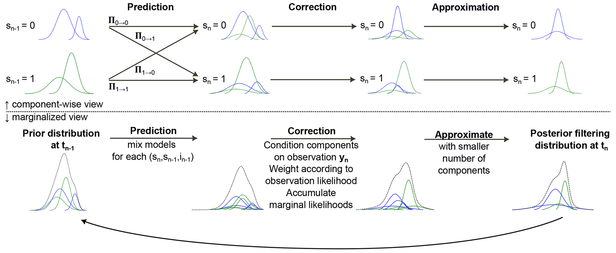
Figure 1Illustration of the iterative computational methods applied in the Gaussian sum filtering (GSF). The filtering distributions (prior and posterior at time steps tn−1 and tn, respectively) are displayed as Gaussian mixtures indexed by in for each of the models indexed by sn. The top panel shows a component-wise view, and the bottom panel shows a marginalized (over sn and in) view of the respective compound distributions. The algorithm can be formally divided into the prediction, correction, and approximation steps. The illustrated iteration starts at some specified prior for t0. For further details, see text and Appendix A2. The output of the algorithm is the approximated decomposed filtering distribution , the input is a prior and a collection of measurements y1:N with associated time stamps, measurement times, and values for all parameters (see text). The approximate marginal likelihood of the measurement sequence can be computed alongside the filtering.
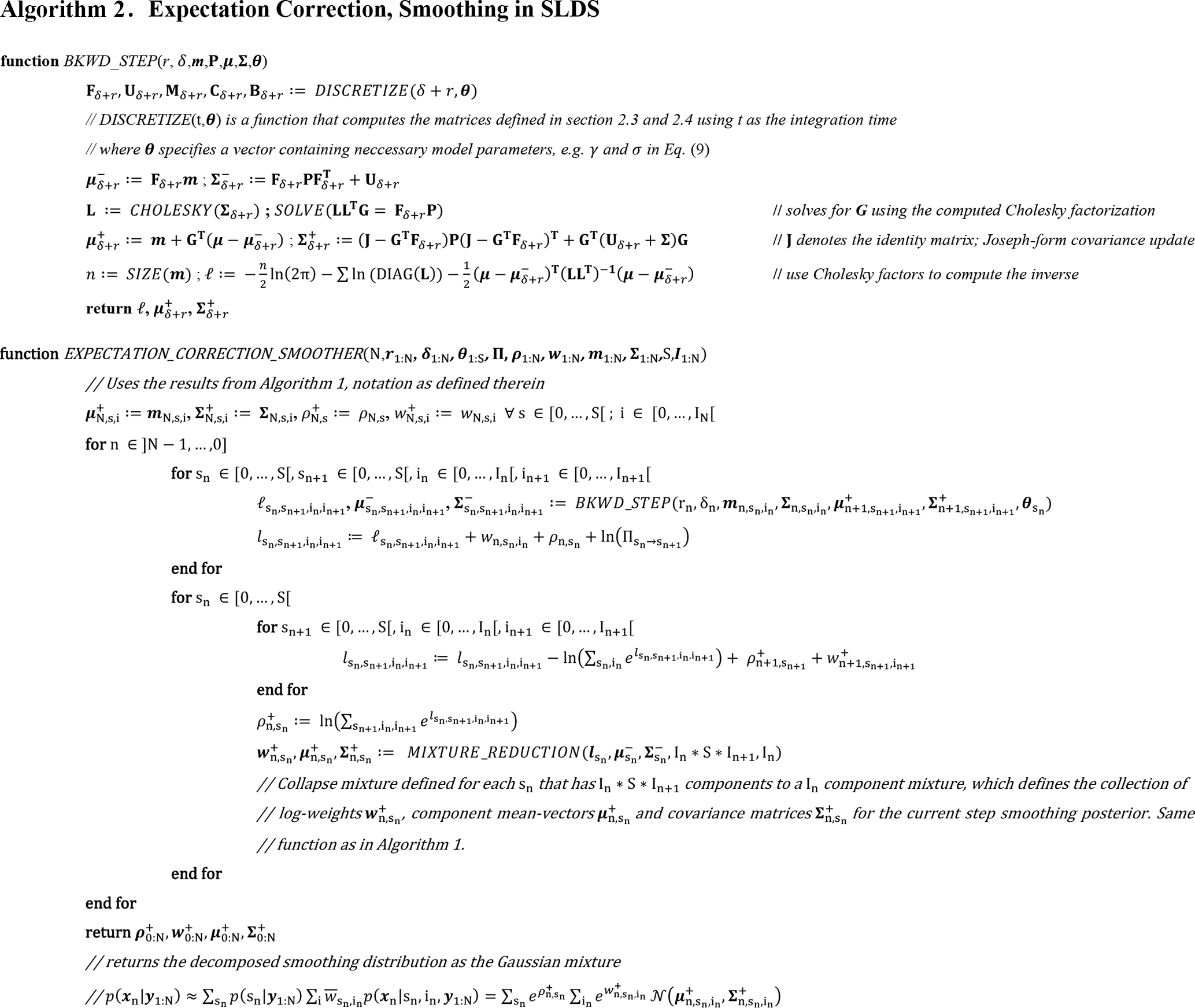
In this setting, the smoothing distribution is also a compound distribution in which the components of each mixture are multiplied within each smoothing step in a backwards recursive formulation by the number of linear dynamical models. Therefore, smoothing is also only possible approximately, once again, on the basis of approximating each arising Gaussian mixture with a smaller one. One way to approximately obtain smoothed results in the SLDS setting is thus given by the expectation correction (EC) algorithm introduced in Barber (2006) and shown therein to provide state-of-the-art results, both in terms of computational efficiency and accuracy, using the results of the GSF forward pass and performing a backwards recursion through the time series. The EC algorithm requires, analogous to the GSF forward pass, the propagation and correction methods, in the form of the filtering and smoothing steps, for the parameterized linear dynamical system outlined in Sect. 2.3 and 2.4 acting on each Gaussian mixture component. In this case, however, the integrating behavior of the measurements does not lead to any required adjustments, and the applied equations are thus exactly analogous to the classical Rauch–Tung–Striebel smoother that represent a formal reversal of the dynamics. These have also been used in the original presentation of the EC algorithm (Algorithm 5 in Barber, 2006). Figure 2 provides a graphical illustration similar to the filtering method in Fig. 1 of the EC smoothing backward pass. The EC algorithm provided in Barber (2006) was used without further modifications, and for more information on this algorithm, the reader is directed to this work.
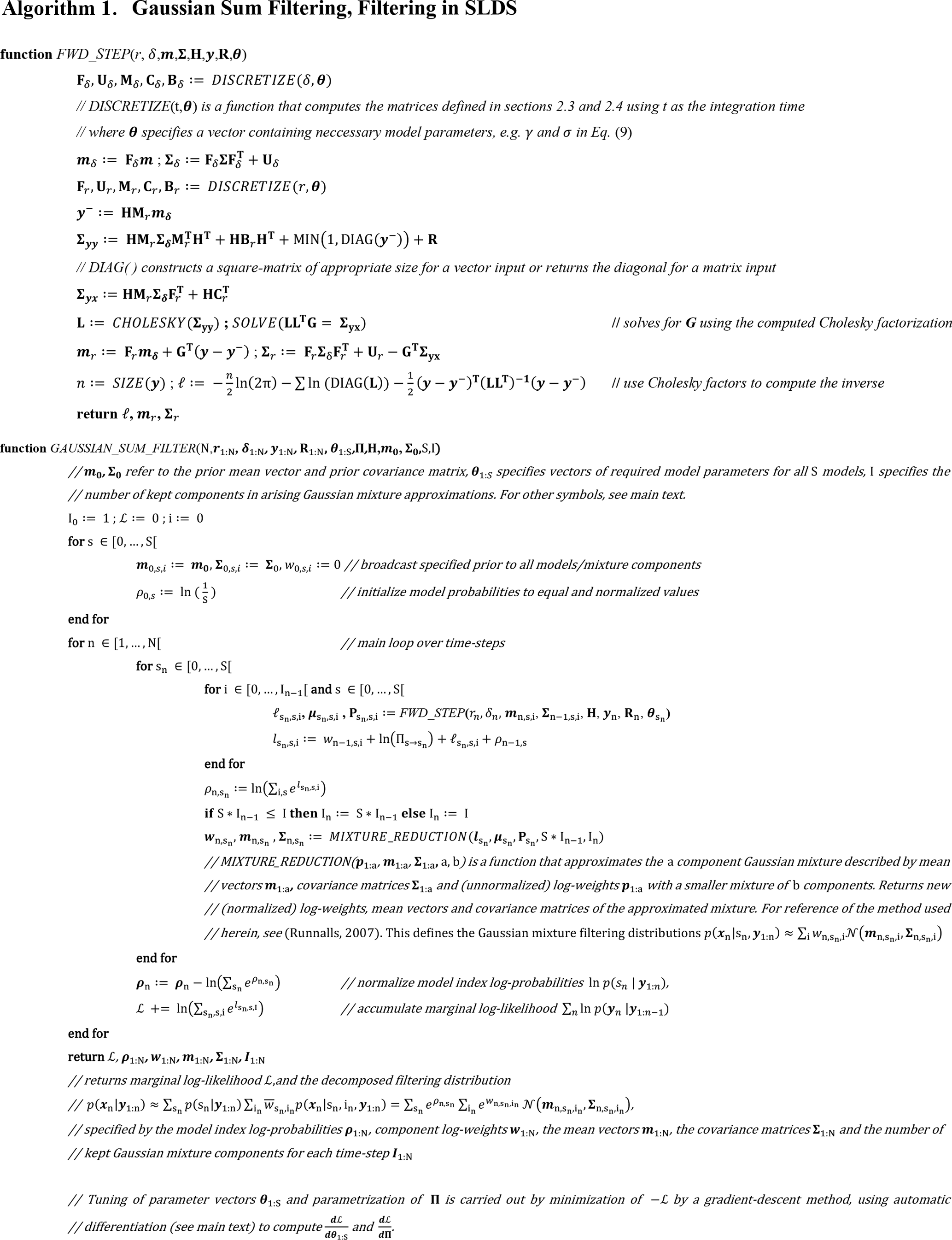
While not a main contribution to this paper, for completeness sake and to facilitate possible re-implementation, both the GSF forward pass and the EC backward pass are outlined in pseudo-code in Appendix A2 in the way they have been implemented here.
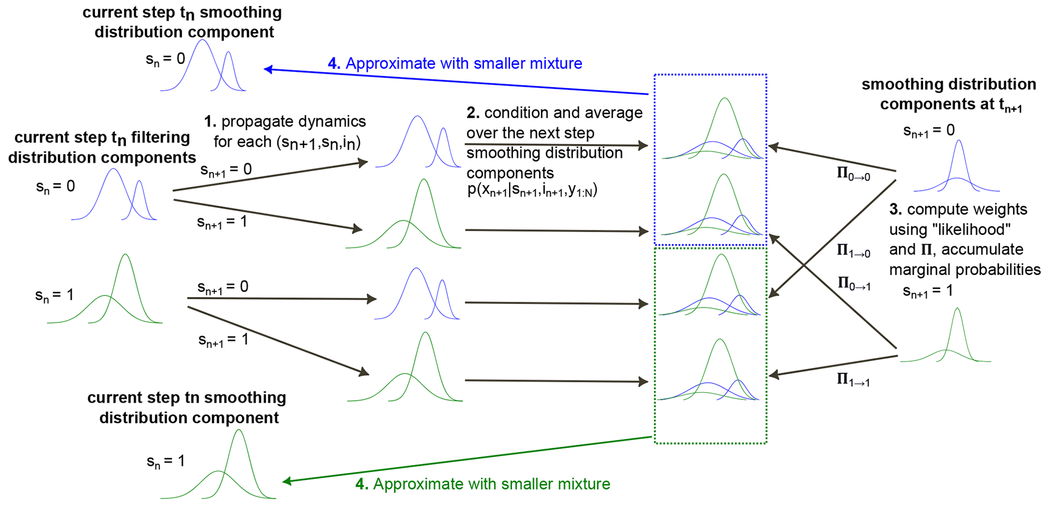
Figure 2Illustration of the backward iterative computational steps (1)–(4) in the expectation correction algorithm applied for correcting the results from the Gaussian sum filtering (GSF) outlined in Fig. 1 to the approximate smoothing solution in the switching linear dynamical system. Input to the algorithm are the results from the GSF and associated time stamps and values for all parameters. Output is the decomposed smoothing distribution as a Gaussian mixture approximation.
To model the two distinct regimes outlined before, two linear dynamical models are used that share their γ values, but for one (cf. Eq. 8), σ is constrained to a small value. Consequently, one of the models corresponds to regimes of changing η and the other to near constant η. This approach allows us via the model index probabilities and obtained from the GSF and the EC algorithms to also probabilistically identify regimes of constant radon emanation within a time series of recorded spectra, even when the retained activity of 222Rn is still in a re-equilibration period, as will be illustrated in the experimental results presented later. In that sense, and by construction of the two models, the model index probabilities can be physically interpreted as the probability of the source to currently have stable emanation characteristics. A non-zero σ acting as a regularization term is, however, still needed in the case of the model corresponding to the constant regimes because otherwise the approximations used within both the GSF and the EC algorithm become numerically unstable. The final model contains four unknown parameters, σ,γ, and the components of Π, which is row-wise normalized and whose components are thus parameterized by two parameters. These four parameters are tuned by minimizing the (approximate) negative marginal log likelihood of the measurement series, , that is accessible in the GSF forward pass (see Algorithm 1 in Appendix A2). For the purposes of this initial investigation, we assume the uncertainty arising from uncertain parameters is negligible in light of the counting statistics, the uncertainty encoded in the prior of the initial state, p(x0), and the components of H.
2.6 Propagation of the detection efficiency uncertainty
In practice, the components of H are not known without uncertainty, and the uncertainty associated with H is the most significant contribution to the combined uncertainty of η in most practical cases. The outlined formalism above is a way to obtain estimates for and or the extended compound distributions and detailed in the previous section, respectively. For notational simplicity, the following is formulated with respect to the single-model case but applies analogously to the SLDS model. Formally, the inclusion of this systematic measurement uncertainty into the filtering or smoothing result, respectively, is given by Eq. (15), which is not tractable.
In the present case, we assume H to be constant with respect to time and that its distribution is known from previous measurements, independent of the collection y1:N. Generally, the uncertainty in H associated with, for example, a prior calibration procedure, can reasonably be described by this approximation, if . This allows rewriting Eq. (15) to obtain Eq. (16); however, the result remains computationally infeasible, since it would require an infinite amount of filtering and smoothing passes.
Thus, in the setting at hand, , the result of Eq. (16) is given as an infinite mixture of Gaussian mixtures with weights proportional to p(H). Our strategy of choice to approximately include the systematic uncertainty associated with H is to replace the infinite mixture by a finite version, i.e., to compute the filtering and smoothing densities for specific realizations of H and combine them into mixtures weighted with the likelihood of said realization under the density p(H) known from prior calibration measurements. In practice, this is closely related to the selection of sigma points of H within some prior density and using the associated normalized likelihoods as multiplicative weights with the respective filtering and smoothing mixture weights to obtain extended mixtures that approximately reflect the uncertainty associated with H, a method inspired by the unscented Kalman filter (Julier et al., 2000) for approximate filtering in non-linear systems.
2.7 Implementation details
Implementation of the presented algorithms was carried out in Python using the JAX framework (Bradburry et al., 2018), which provides automatic batching and vectorization, just-in-time compilation, and automatic forward- and reverse-mode differentiation. This allows the optimization of the hyperparameters γ, σ, and Π using the ADAM gradient descent minimization (Kingma and Ba, 2014) routine from JAX together with the automatically computed batch gradient of the negative log likelihood, , of the GSF forward pass on the entire dataset (Algorithm 1 in Appendix A2). The number of components retained in the arising Gaussian mixtures in GSF and EC is chosen according to available computational resources. Forward and backward step routines for the linear dynamical system given in Eq. (2) (cf. Appendix A1) were implemented as shown in the auxiliary functions for Algorithms 1 and 2 in Appendix A2, respectively. Gaussian mixture reduction as necessary in the GSF forward and EC backward passes (i.e., the approximation steps in the charts in Figs. 1 and 2) was implemented according to a greedy algorithm (based on Kullback–Leibler divergence (Runnalls, 2007). The mean approximation in the EC backward pass, and implementation of the EC backward and GSF forward passes, were directly adopted as presented in Barber (2006). Gaussian mixture weights and model index probabilities are stored and operated on in ln-space (using the log-sum-exp operation for normalization) for improved numerical stability. Routines for the computation of the Matrices F, U, M, C, and B in Eq. (13) were obtained from symbolic computation using SymPy (Meurer et al., 2017), and the symbolic Jordan canonical form of F and were hardcoded afterward.
Data for this experiment were generated using an electroplated 226Ra (104.4±0.4) Bq source (Mertes et al., 2020) mounted on an electrically cooled high-purity germanium (HPGe) detector placed inside a 20 m3 climate chamber. γ-ray spectra were recorded over approximately 85 d at intervals of 10 800 s real time. Within the time series, regions of missing measurements are present, i.e., δ values varied. At specific times the relative humidity inside the climate chamber was varied with the intention of inducing changes in the emanation characteristics of the 226Ra source. Inside the chamber, relative humidity and temperature were measured in close proximity to the source with a SHT-35 sensor (Sensirion).
For each spectrum, counts above 200 keV were summed, a lifetime scaled background count rate (with associated uncertainty that defines R) was subtracted, and the final algorithms described above (as given in Appendix A2) were applied to the resultant time series of count values (i.e., 1D measurement series) as the input data y1:N, with five Gaussian components per filter in the GSF forward and EC backward passes. Results are illustrated for the filtering in Fig. 1a and for the smoothing in Fig. 1b. Each r was chosen to reflect the real time of each spectrum as provided by the manufacturer's data-acquisition software (Genie 2000, Mirion Technologies), and each δ was computed from the recorded time stamps of acquisition start points. The dead time of the system was accounted for by correcting the derived count values using the dead-time data as provided by the data-acquisition software. The value of H was determined by measurements of a sealed source of similar type and geometry as presented in Mertes et al. (2020). The uncertainty associated with the 226Ra activity known from previous measurements detailed in Mertes et al. (2020) was encoded in the density of the prior for the state provided to the algorithm. Apart from the 226Ra activity, a vague Gaussian prior with a diagonal covariance matrix was chosen for p(x0). Inherently, the model formulation assumes perfect equilibrium between the SLP and 222Rn in the source, which is a small approximation on the timescales at hand. The threshold of 200 keV was chosen because 226Ra emits γ radiation almost entirely below this energy level, such that the spectrum beyond is almost entirely made up of events associated with the SLP in the source and the background radiation. We chose to neglect the information gained from the spectra regarding the 226Ra activity because it was not found to substantially improve the prior. The summation of spectra is the most straightforward way to utilize the information contained within each spectrum while keeping the dimensionality of y as small as possible. As a result, the prior density for the 226Ra activity component of the state is retained over the entire dataset, which is why this component of the state is not shown in Fig 3. The last component of the state vectors, , is also not shown in Fig. 3 for visual clarity, since it carries no important information and is merely used as a mathematical tool to specify the properties of the stochastic process of η, the main estimation target of this work. The component is therefore not of any practical meaning.
Both the confidence intervals and the median in Fig. 3 were computed from the marginal cumulative density of the Gaussian mixtures using numerical root finding. Additionally, the confidence intervals include a systematic, Gaussian 1 % uncertainty on the specific value of H which was approximately propagated using the derivation in Sect. 2.6 for five distinct realizations of H ().
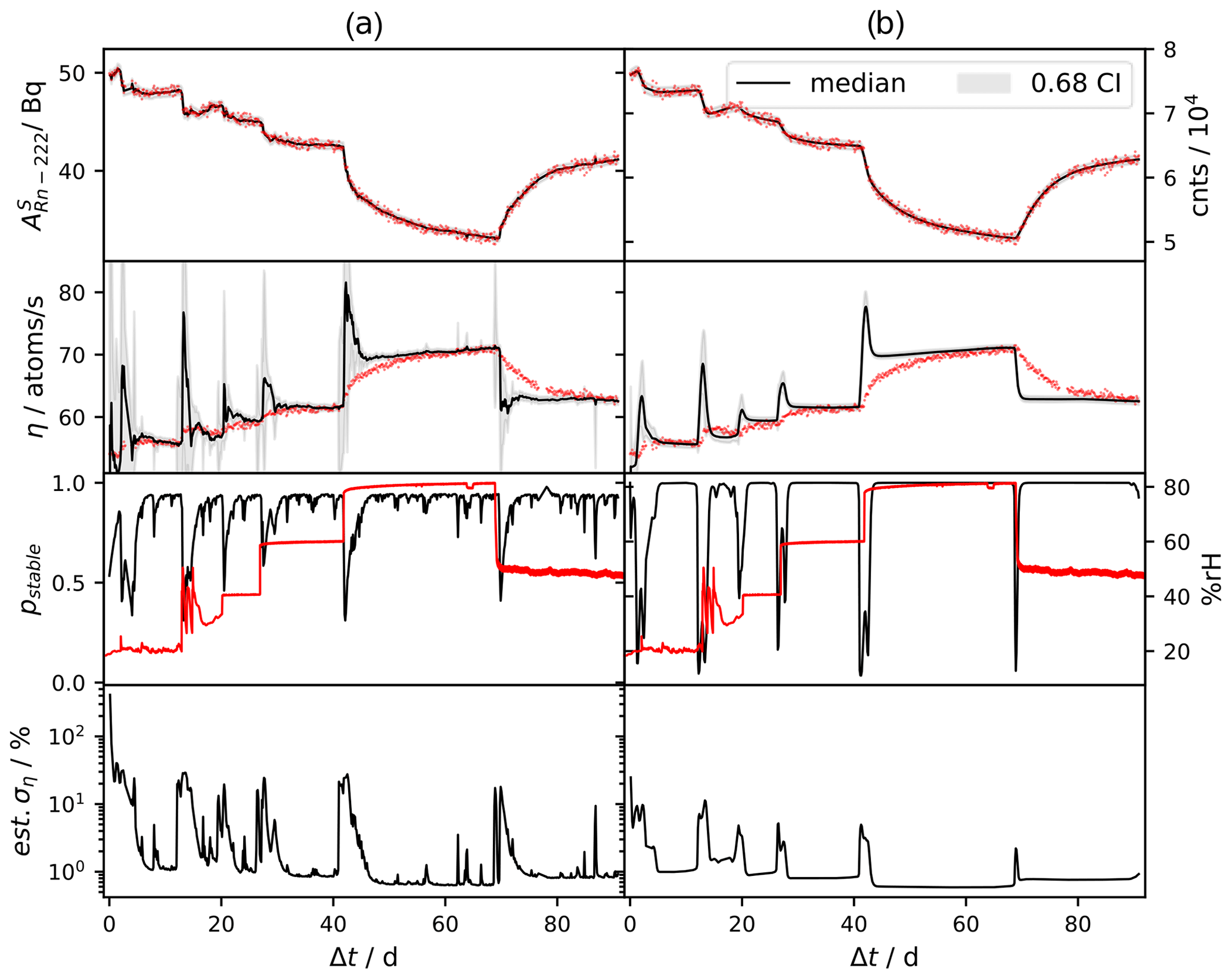
Figure 3Column (a) shows the filtering and column (b) the smoothing results. Input data (red dots in the top-most row; right scale) and estimated residual 222Rn activity (left scale) are depicted in the first row. The second row shows the estimated emanating 222Rn given by the SLDS deconvolution approach outlined in Sect. 2.5 (black line; deconvolution result) and erroneously calculated from Eq. (4) (red dots). Deviations between the red dots and the filtering and smoothing results in row two are due to the inability of Eq. (4) to account for dynamic behavior. In the third row, the probability for stable regimes under the model, (column a), and (column b), where sn equals the index of the model for the stable regime (black; i.e., inferred switch points; see Sect. 2.7) and the relative humidity (red; not used as input data) are shown. The fourth row shows the estimated relative standard uncertainty (calculated from the median and the shown confidence interval) of inferred 222Rn emanation.
In the present work, we have summarized and explained the limitations of previously available approaches to estimate 222Rn emanation through measurements of the short-lived progeny (SLP) retained within the source. As was derived from first principles, those methods to standardize 222Rn emanation are limited to sources with stable characteristics within the operational time and, as such, are generally restricted to use in stable environmental conditions. To alleviate this shortcoming, here we developed an alternative approach that directly infers the conditional probability density for the latent 222Rn emanation term from spectral time series of the SLP that remains within the source.
During the application of the resultant algorithms to real-world data, the deviations of the steady-state approximation of the previous method (red dots in the second row of Fig. 3) from the estimated true values (black lines in the second row of Fig. 3) become apparent, underpinning the theoretical derivations. In turn, this means that a thorough analysis of data obtained in this way is restricted to models that account for the dynamic nature of the system, which has not previously been reported.
The specific structure of the filtering and smoothing results in the second row of Fig. 3, showing peaked emanation upon increases in humidity, can easily be explained physically as follows, which justifies the results of the applied method. Considering the time series of count data of the SLP within the source (input data; red dots in the first row of Fig. 3), regions can be seen where changes are occurring much more quickly than would be possible based on the well-known radioactive decay kinetics. As was discussed in Sect. 2.2, the time series of counts is theoretically given by a discretely sampled convolved version of the emanation. Hence, peaked emanation must be occurring, such that the observed time series is possible within the theoretically known decay kinetics. Conversely, the drop in humidity and thus emanation at approximately 70 d does not show this behavior, and the observed ingrowth of the counts directly follows the decay kinetics. Apparently, the behavior depends on the direction of change in the emanation characteristics. This is explained by the fact that upon an increase of the effective diffusion coefficient, the source retains more 222Rn atoms than the associated equilibrium value, at which point increased outflow can occur for quick re-equilibration. With the realistic assumption of zero back diffusion from the volume into the source, for a change in the opposite direction, the only way to achieve progeny equilibrium is the typical ingrowth of 222Rn, which is the exact behavior shown by the deconvolution result but not by the previous method. Upon fresh preparation of an emanation source, at which point no SLP is present in the source but emanation is still considered to be happening, similar count data to the one past 70 d in Fig. 3 may be observed. This behavior was not previously discussed in Linzmaier and Röttger (2013), where the apparent initial drop in emanation (as computed by Eq. 4) resulting from the initial ingrowth of residual 222Rn and SLP was seemingly considered to be its true temporal characteristic, implying that Eq. (4) may be applied in such a case.
In constant regimes, results obtained from previously reported methods converge to the values obtained using the deconvolution approach presented here, as illustrated at approximately days 60 to 70 and past 90 d of the data shown in Fig. 3. While the method we present might not seem beneficial in such constant regimes, the recursive Bayesian approach provides a computationally convenient, mathematically coherent, and flexible way to refine the uncertainty upon observation of streaming data (e.g., obtained by continuous operation of spectrometers) also within constant regimes. As such, here we report for the first time the application of a method whereby time series data of an emanation source can be used to derive correct (near) real time values of the emanation, irrespective of the state of the source. Specifically, the use case of this method and our initial motivation is the implementation of surveillance systems for emanation sources based on spectrometric measurements to improve current state-of-the-art realization, and especially the dissemination of the unit Bq m−3 for 222Rn in the low-level activity concentration regime. With our contribution, and potential extensions thereof, these types of systems will be enabled in the future. Moreover, experimental investigations of the emanation behavior in response to different environmental conditions are drastically improved by our contribution.
To obtain approximate filtering and smoothing algorithms in the context of radioactivity measurements, we extended the well-known computational methods for inference in linear dynamical systems (i.e., Kalman filter and Rauch–Tung–Striebel smoother) with a computationally convenient approximation for the observed Poisson statistics and the integrating behavior of the measurements in Sect. 2.3 and 2.4. In doing so, we demonstrated that integrating measurements results in a Gaussian process with certain covariance with the latent continuous state which retains the convenient closed form of filtering and smoothing through conjugacy in such linear dynamical models. As was shown, the integrating measurements lead to additional additive uncertainty depending on the variance of the Brownian motion which we consider an intuitive result. These results were used in order to construct the final switching linear dynamical system inference algorithms applied during the experiments.
Within the recorded time series, distinct domains were observed in response to the way the humidity in the chamber was modified, which lends itself to the applied switching dynamical system model, differentiating between stable and non-stable regimes. This approach allows smaller uncertainty to be achieved and smoother functional realizations of η in the somewhat stable regimes, but at the same time gives reasonably high uncertainty for the unstable regimes where the deconvolution result relies on only a few data points. A simpler modeling approach relying only on a single linear dynamical system, such as a more classical version of the Kalman filter, cannot produce smooth results for the constant regimes while retaining the ability to react to steep gradients, since both properties are controlled by the variance of the Brownian motion. While all obvious switching points (induced by changes in the relative humidity) within the time series were captured by the algorithm (third row of Fig. 3), the specific autocorrelation we chose to regularize η leads to smearing of the switching point in the backward (i.e., the smoothing) pass. This is indicated by the fact that the model proposes an unstable state of the source even for times before the humidity has undergone the step changes (i.e., in times before a known change in the source properties has occurred). Note that this is not the case for the filtering results. This is can be attributed to the applied symmetric autocorrelation of η (Eq. 7) and its independency from the residual radon activity, and it may be alleviated by asymmetric autocorrelation or non-linear models but at a substantially higher computational cost. Whether our approach translates well to time series of different characteristics (e.g., drift, smooth changes) is as yet unclear and subject to further studies. Nonetheless, the model parameters provide a way to tune the algorithm for different scenarios.
For an approach like the present one to be applicable in metrology, uncertainty estimates closely related to the guide to the expression of uncertainty in measurement (GUM; Joint Committee for Guides in Metrology, 2008) are needed. At this point, the GUM is restricted to static measurements and first steps are being taken for an extension to dynamic scenarios (e.g., in Eichstädt and Elster, 2012; Elster and Link, 2008; Link and Elster, 2009), where a slightly different formulation for error propagation has been carried out. In the present case, systematic contributions to the uncertainty are dominated by the uncertainty of the measurement mapping through matrix H. We provided a computationally simple approach to approximately propagate this uncertainty across the filtering and smoothing algorithms with arbitrary precision, given that enough computational resources are available and the detection system can reasonably be assumed to be stable in time. Dropping this assumption would require the approximation of the intractable integration in Eq. (15), e.g., through Monte Carlo integration, which was found unnecessary and would have made the algorithm unsuitable for implementation on low-power, portable devices.
Assuming that the density is given as , we define the state at the intermediate time point as xδ for which the following statistics are readily available through the Chapman–Kolmogorov equation (Särkkä and Solin, 2019).
where Fδ=eKδ and , as follows from Eqs. (5) and (11).
By combination of the definition for x(t) in Eq. (10) and the definition of the measurement process for y in Eq. (12), the measurement at tn is given by the following integration. While the integral in Eq. (12) is an ordinary integral (e.g., in the Riemann sense), the integral in Eq. (10) is a stochastic integral in the Itō sense; i.e., the following double integral is the ordinary integral over an Itō integral, for which we assume that x(t) has continuous sample paths and is square integrable.
The triangular domain of the double integral is swapped to find
from which the full density can be computed using the expectation operator and the definition of the variance, where 〈⋅〉 denotes the expectation operator. Moreover, by definition, and thus
Under the assumption of independence of the Brownian motion and xδ, using Itō isometry and Fubini's theorem, it follows that
where and .
Analogously, the cross-covariance between xn and yn is given as
with . The result in Eq. (13) is then obtained by marginalizing the full density over xn−1 and xδ, which for the Gaussian density means to simply drop the respective columns and rows. Additionally, the forward filtering step is obtained by conditioning the resultant , Eq. (13), onto the observation of yn using the well-known conditioning formula for the Gaussian distribution. An implementation for such computation is given by the function FWD_STEP in Appendix A2.
Gamma-ray spectra and environmental data obtained for the experimental section as well as the implementation of the presented algorithms and processing software are available at https://doi.org/10.5281/zenodo.7798458 (Mertes, 2023).
AR and SR acquired funding, supervised and conceptualized this work, and reviewed the draft. FM derived the methodology, designed the models, implemented the software, acquired the experimental data, and prepared the original draft.
The contact author has declared that none of the authors has any competing interests.
Publisher’s note: Copernicus Publications remains neutral with regard to jurisdictional claims in published maps and institutional affiliations.
This article is part of the special issue “Sensors and Measurement Science International SMSI 2021”. It is a result of the Sensor and Measurement Science International, 3–6 May 2021.
The authors thank Alan Griffiths (ANSTO) and Scott D. Chambers (ANSTO) for their comments on the paper.
This project has received funding from the EMPIR programme co-financed by
the Participating States and from the European Union's Horizon 2020 research
and innovation programme. 19ENV01 traceRadon denotes the EMPIR project
reference.
This open-access publication was funded by the Physikalisch-Technische Bundesanstalt.
This paper was edited by Alexander Bergmann and reviewed by two anonymous referees.
Alvarez, M., Luengo, D., and Lawrence, N. D.: Latent force models, J. Mach. Learn. Res., 5, 9–16, 2009.
Amaku, M., Pascholati, P. R., and Vanin, V. R.: Decay chain differential equations: Solution through matrix algebra, Comput. Phys. Commun., 181, 21–23, https://doi.org/10.1016/j.cpc.2009.08.011, 2010.
Barber, D.: Expectation Correction for Smoothed Inference in Switching Linear Dynamical Systems, J. Mach. Lear. Res., 2, 2515–2540, 2006.
Bateman, H.: Solution of a system of differential equations occuring in the theory of radioactive transformations, P. Cam. Philos. Soc., 15, 423–427, 1910.
Biraud, S., Ciais, P., Ramonet, M., Simmonds, P., Kazan, V., Monfray, P., O'doherty, S., Spain, G., and Jennings, S. G.: Quantification of carbon dioxide, methane, nitrous oxide and chloroform emissions over Ireland from atmospheric observations at Mace Head, Tellus B, 54, 41–60, https://doi.org/10.3402/tellusb.v54i1.16647, 2002.
Bradburry, J., Frostig, R., Hawkins, P., Johnson, M. J., Maclaurin, D., Necula, G., Paszke, A., van der Plas, J., Wanderman-Milne, S., and Zhang, Q.: JAX: composable transformations of Python+Numpy programs, GitHub [code], https://github.com/google/jax (last access: 1 April 2023), 2018.
Chambers, S., Podstawczyńska, A., Pawlak, W., Fortuniak, K., Williams, A. G., and Griffiths, A. D.: Characterizing the State of the Urban Surface Layer Using Radon-222, J. Geophys. Res.-Atmos., 124, 770–788, https://doi.org/10.1029/2018JD029507, 2019a.
Chambers, S., Guérette, E.-A., Monk, K., Griffiths, A., Zhang, Y., Duc, H., Cope, M., Emmerson, K., Chang, L., Silver, J., Utembe, S., Crawford, J., Williams, A., and Keywood, M.: Skill-Testing Chemical Transport Models across Contrasting Atmospheric Mixing States Using Radon-222, Atmosphere, 10, 25, https://doi.org/10.3390/atmos10010025, 2019b.
Chambers, S. D., Williams, A. G., Conen, F., Griffiths, A. D., Reimann, S., Steinbacher, M., Krummel, P. B., Steele, L. P., van der Schoot, M. V., Galbally, I. E., Molloy, S. B., and Barnes, J. E.: Towards a Universal “Baseline” Characterisation of Air Masses for High- and Low-Altitude Observing Stations Using Radon-222, Aerosol. Air Qual. Res., 16, 885–899, https://doi.org/10.4209/aaqr.2015.06.0391, 2016.
Chambers, S. D., Preunkert, S., Weller, R., Hong, S.-B., Humphries, R. S., Tositti, L., Angot, H., Legrand, M., Williams, A. G., Griffiths, A. D., Crawford, J., Simmons, J., Choi, T. J., Krummel, P. B., Molloy, S., Loh, Z., Galbally, I., Wilson, S., Magand, O., Sprovieri, F., Pirrone, N., and Dommergue, A.: Characterizing Atmospheric Transport Pathways to Antarctica and the Remote Southern Ocean Using Radon-222, Front. Earth Sci., 6, 190, https://doi.org/10.3389/feart.2018.00190, 2018.
Darby, S., Hill, D., Auvinen, A., Barros-Dios, J. M., Baysson, H., Bochicchio, F., Deo, H., Falk, R., Forastiere, F., Hakama, M., Heid, I., Kreienbrock, L., Kreuzer, M., Lagarde, F., Mäkeläinen, I., Muirhead, C., Oberaigner, W., Pershagen, G., Ruano-Ravina, A., Ruosteenoja, E., Rosario, A. S., Tirmarche, M., Tomáscaron;ek, L., Whitley, E., Wichmann, H.-E., and Doll, R.: Radon in homes and risk of lung cancer: collaborative analysis of individual data from 13 European case-control studies, BMJ, 330, 223, https://doi.org/10.1136/bmj.38308.477650.63, 2005.
Ebeigbe, D., Berry, T., Schiff, S. J., and Sauer, T.: Poisson Kalman filter for disease surveillance, Phys. Rev. Res., 2, 043028, https://doi.org/10.1103/PhysRevResearch.2.043028, 2020.
Eichstädt, S. and Elster, C.: Advanced Mathematical and Computational Tools in Metrology and Testing IX, 84, 126–135, https://doi.org/10.1142/9789814397957_0016, 2012.
Elster, C. and Link, A.: Uncertainty evaluation for dynamic measurements modelled by a linear time-invariant system, Metrologia, 45, 464–473, https://doi.org/10.1088/0026-1394/45/4/013, 2008.
Fialova, E., Otahal, P. P. S., Vosahlik, J., and Mazanova, M.: Equipment for Testing Measuring Devices at a Low-Level Radon Activity Concentration, Int. J. Environ. Res. Pub. He., 17, 1904, https://doi.org/10.3390/ijerph17061904, 2020.
Hartikainen, J. and Särkkä, S.: Sequential Inference for Latent Force Models, arXiv [preprint], https://doi.org/10.48550/arXiv.1202.3730, 2012.
Janik, M., Omori, Y., and Yonehara, H.: Influence of humidity on radon and thoron exhalation rates from building materials, Appl. Radiat. Isotopes, 95, 102–107, https://doi.org/10.1016/j.apradiso.2014.10.007, 2015.
Joint Committee for Guides in Metrology: Evaluation of measurement data – Supplement 1 to the, JCGM 101, 90, https://www.bipm.org/documents/20126/2071204/JCGM_101_2008_E.pdf/325dcaad-c15a-407c-1105-8b7f322d651c (last access: 1 April 2023), 2008.
Julier, S., Uhlmann, J., and Durrant-Whyte, H. F.: A new method for the nonlinear transformation of means and covariances in filters and estimators, IEEE T. Automat. Contr., 45, 477–482, https://doi.org/10.1109/9.847726, 2000.
Kalman, R. E.: A New Approach to Linear Filtering and Prediction Problems, J. Basic Eng.-T. ASME, 82, 35–45, https://doi.org/10.1115/1.3662552, 1960.
Kingma, D. P. and Ba, J.: Adam: A Method for Stochastic Optimization, arXiv [preprint], https://doi.org/10.48550/arXiv.1412.6980, 2014.
Laan, V. Der, Karstens, U., Neubert, R. E. M., Laan-Luijkx, V. Der, and Meijer, H. A. J.: Observation-based estimates of fossil fuel-derived CO2 emissions in the Netherlands using Δ14C, CO and 222Radon, Tellus B, 62, 389–402, https://doi.org/10.1111/j.1600-0889.2010.00493.x, 2010.
Levin, I.: Atmospheric CO2 in continental Europe-an alternative approach to clean air CO2 data, Tellus B, 39, 21–28, https://doi.org/10.1111/j.1600-0889.1987.tb00267.x, 1987.
Levin, I., Karstens, U., Hammer, S., DellaColetta, J., Maier, F., and Gachkivskyi, M.: Limitations of the radon tracer method (RTM) to estimate regional greenhouse gas (GHG) emissions – a case study for methane in Heidelberg, Atmos. Chem. Phys., 21, 17907–17926, https://doi.org/10.5194/acp-21-17907-2021, 2021.
Levy, E.: Decay chain differential equations: Solutions through matrix analysis, Comput. Phys. Commun., 234, 188–194, https://doi.org/10.1016/j.cpc.2018.07.011, 2019.
Link, A. and Elster, C.: Uncertainty evaluation for IIR (infinite impulse response) filtering using a state-space approach, Meas. Sci. Technol., 20, 055104, https://doi.org/10.1088/0957-0233/20/5/055104, 2009.
Linzmaier, D. and Röttger, A.: Development of a low-level radon reference atmosphere, Appl. Radiat. Isotopes, 81, 208–211, https://doi.org/10.1016/j.apradiso.2013.03.032, 2013.
Mazor, E., Averbuch, A., Bar-Shalom, Y., and Dayan, J.: Interacting multiple model methods in target tracking: a survey, IEEE T. Aerospace Elec. Sys., 34, 103–123, https://doi.org/10.1109/7.640267, 1998.
Mertes, F.: FlorianMertes/RadonDeconvolution: Version 1.0 (Release), Zenodo [code] and [data set], https://doi.org/10.5281/zenodo.7798458, 2023.
Mertes, F., Röttger, S., and Röttger, A.: A new primary emanation standard for Radon-222, Appl. Radiat. Isotopes, 156, 108928, https://doi.org/10.1016/j.apradiso.2019.108928, 2020.
Meurer, A., Smith, C. P., Paprocki, M., Čertík, O., Kirpichev, S. B., Rocklin, M., Kumar, Am., Ivanov, S., Moore, J. K., Singh, S., Rathnayake, T., Vig, S., Granger, B. E., Muller, R. P., Bonazzi, F., Gupta, H., Vats, S., Johansson, F., Pedregosa, F., Curry, M. J., Terrel, A. R., Roučka, Š., Saboo, A., Fernando, I., Kulal, S., Cimrman, R., and Scopatz, A.: SymPy: symbolic computing in Python, PeerJ Computer Science, 3, e103, https://doi.org/10.7717/peerj-cs.103, 2017.
Minka, T. P.: Expectation Propagation for approximate Bayesian inference, arXiv [preprint], https://doi.org/10.48550/arXiv.1301.2294, 2013.
Nadarajah, N., Tharmarasa, R., McDonald, M., and Kirubarajan, T.: IMM Forward Filtering and Backward Smoothing for Maneuvering Target Tracking, IEEE T. Aero. Elec. Sys., 48, 2673–2678, https://doi.org/10.1109/TAES.2012.6237617, 2012.
Perrino, C., Pietrodangelo, A., and Febo, A.: An atmospheric stability index based on radon progeny measurements for the evaluation of primary urban pollution, Atmos. Environ., 35, 5235–5244, https://doi.org/10.1016/S1352-2310(01)00349-1, 2001.
Pressyanov, D. S.: Short solution of the radioactive decay chain equations, Am. J. Phys., 70, 444–445, https://doi.org/10.1119/1.1427084, 2002.
Rauch, H. E., Tung, F., and Striebel, C. T.: Maximum likelihood estimates of linear dynamic systems, AIAA J., 3, 1445–1450, https://doi.org/10.2514/3.3166, 1965.
Röttger, A., Honig, A., and Linzmaier, D.: Calibration of commercial radon and thoron monitors at stable activtiy concentrations, Appl. Radiat. Isotopes, 87, 44–47, https://doi.org/10.1016/j.apradiso.2013.11.111, 2014.
Runnalls, A. R.: Kullback-Leibler Approach to Gaussian Mixture Reduction, IEEE T. Aero. Elec. Sys., 43, 989–999, https://doi.org/10.1109/TAES.2007.4383588, 2007.
Särkkä, S.: Bayesian filtering and smoothing, Cambridge University Press, https://doi.org/10.1017/CBO9781139344203, 2013.
Särkkä, S. and Solin, A.: Applied Stochastic Differential Equations, Cambridge University Press, https://doi.org/10.1017/9781108186735, 2019.
Särkkä, S., Alvarez, M. A., and Lawrence, N. D.: Gaussian Process Latent Force Models for Learning and Stochastic Control of Physical Systems, IEEE T. Automat. Contr., 64, 2953–2960, https://doi.org/10.1109/TAC.2018.2874749, 2019.
Stranden, E., Kolstad, A. K., and Lind, B.: The Influence of Moisture and Temperature on Radon Exhalation, Radiat. Prot. Dosim., 7, 55–58, https://doi.org/10.1093/oxfordjournals.rpd.a082962, 1984.
Williams, A. G., Chambers, S., and Griffiths, A.: Bulk Mixing and Decoupling of the Nocturnal Stable Boundary Layer Characterized Using a Ubiquitous Natural Tracer, Bound.-Lay. Meteorol., 149, 381–402, https://doi.org/10.1007/s10546-013-9849-3, 2013.
Williams, A. G., Chambers, S. D., Conen, F., Reimann, S., Hill, M., Griffiths, A. D., and Crawford, J.: Radon as a tracer of atmospheric influences on traffic-related air pollution in a small inland city, Tellus B, 68, 30967, https://doi.org/10.3402/tellusb.v68.30967, 2016.
Zhou, Q., Shubayr, N., Carmona, M., Standen, T. M., and Kearfott, K. J.: Experimental study of dependence on humidity and flow rate for a modified flowthrough radon source, J. Radioanal. Nucl. Ch., 324, 673–680, https://doi.org/10.1007/s10967-020-07081-0, 2020.
- Abstract
- Introduction
- Theory and derivations
- Application to experimental data
- Discussion and conclusion
- Appendix A: Joint density – derivation of discrete forward step for integrating measurement
- Appendix B: Applied algorithms in pseudo-code
- Code and data availability
- Author contributions
- Competing interests
- Disclaimer
- Special issue statement
- Acknowledgements
- Financial support
- Review statement
- References