the Creative Commons Attribution 4.0 License.
the Creative Commons Attribution 4.0 License.
 | 16 Nov 2023
Wireless surface acoustic wave resonator sensors: fast Fourier transform, empirical mode decomposition or wavelets for the frequency estimation in one shot?
Angel Scipioni
Pascal Rischette
Agnès Santori
Most applications which measure physical quantities, especially in harsh environments, rely on surface acoustic wave resonators (SAWRs). Measuring the variation of the resonance frequency is a fundamental step in such cases. This article presents a comparison between three techniques for best determining the resonance frequency in one shot from the point of accuracy and uncertainty: fast Fourier transform (FFT), discrete wavelet transform (DWT) and empirical mode decomposition (EMD). After proposing a model for the generation of synthetic SAW signals, the question of wavelet choice is answered. The three techniques are applied to synthetic signals with different central frequencies and signal-to-noise ratios (SNRs). They are also tested on experimental signals with different sampling rates, number of samples and SNRs. Results are discussed in terms of the accuracy of the estimated frequency and measurement uncertainty. This study is successfully extended to SAWR temperature sensors.
- Article
(20072 KB) - Full-text XML
- BibTeX
- EndNote


For some years now, the industry has been experiencing a strong trend in the integration of preventive maintenance in its development strategy (Lee et al., 2014). The drastic control of operation and investment costs requires a permanent optimization of proper working conditions of production machines. Therefore, the diagnostics of several physical quantities, such as vibration, is experiencing considerable growth in the field of aeronautics or rotating electrical machines (ISO 2372, 10816) (Scheffer and Girdhar, 2004; Brandt, 2011). Temperature monitoring, especially in harsh environments (François et al., 2015, 2012), also poses a major challenge in countless applications (Kim et al., 2015; Li et al., 2014), and this is precisely the focus of this study. These diagnostics are increasingly based on surface acoustic wave (SAW) devices that are now well established in research (Han et al., 2021; Nguyen et al., 2017) and in the industry (Pohl, 2000; Hadj-Larbi and Serhane, 2019). Their operation principles make them almost indispensable: this is why they are found particularly in temperature (Lamanna et al., 2020; Silva et al., 2017), humidity (Li et al., 2014; Penza and Cassano, 2000), torque (Kalinin et al., 2013), magnetic field (Li et al., 2014), strain (Maskay et al., 2018), mass (Tadigadapa and Mateti, 2009) or vibration (Wang et al., 2014) sensors.
A major advantage of this kind of sensor is its ability to act discreetly. It does not need any dedicated energy to operate because it picks up its energy from the wave that interrogates it. Thus, a wireless SAW device is completely passive and able to operate in harsh environments.
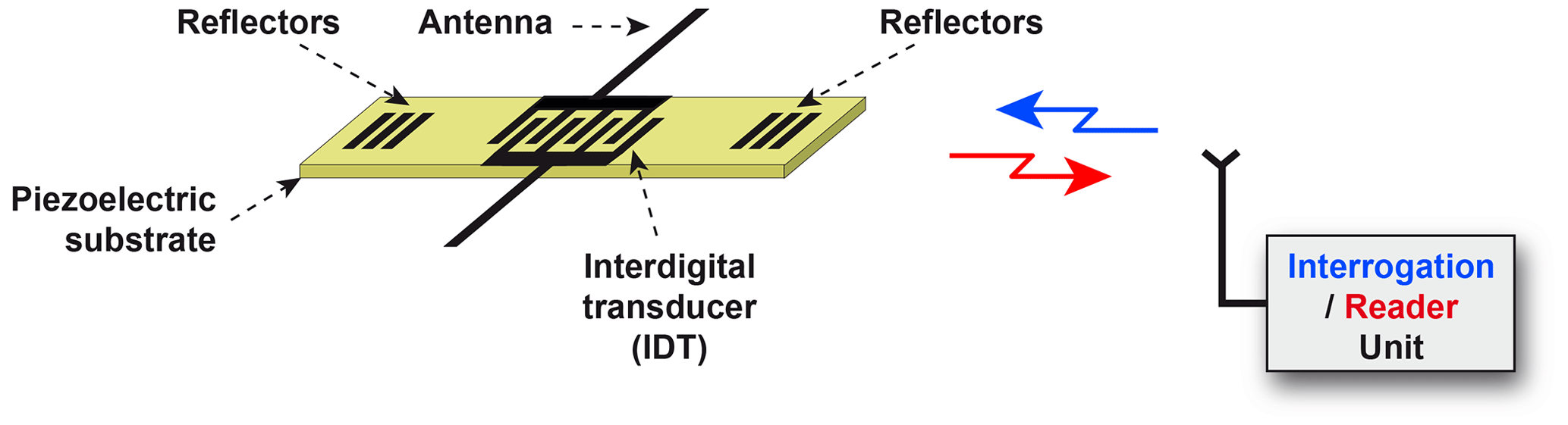
Figure 1 depicts the principle of the wireless SAW sensor on which this work is based. An interdigital transducer (IDT) is insonified by an interrogation or reader unit via an antenna. In a single-port SAW resonator (SAWR), two reflector arrays, which act as a mirror, are placed on either side of the bidirectional IDT. The SAW piezoelectric substrate is warped by mechanical waves due to the physical quantity variation. This deformation causes a modification in the propagation of the surface acoustic wave which is received by the IDT. The propagation change leads to an alteration of the resonance frequency. This variation is directly related to the amplitude of the variation of the considered physical quantity, which in this case is temperature.
In most cases, the fast Fourier transform (FFT) method is applied with its possible variations (zero crossing, zero padding, peak detection, etc.) (Hamsch et al., 2004; Lurz et al., 2017; Jazini et al., 2018). The main drawback of these spectral approaches is the measurement inaccuracy. Its improvement is often obtained by an average of the results (Kalinin et al., 2012) and, in fact, the measurement cannot be done in one shot.
The objective of the work described in this paper is to proceed, in one shot as precisely as possible, with the resonance frequency estimation of the SAWR by comparing three methods: on the one hand the FFT and on the other hand two time-based methods, wavelets (Antoniadis, 2007) and empirical mode decomposition (EMD) (Kizilkaya et al., 2015).
This article is an in-depth study of a conference contribution (Scipioni et al., 2019). It is structured in four parts with all theoretical elements in Appendix A and notations in Appendix B. After the introduction, Sect. 2 is dedicated to a presentation of the methods. A theoretical model for the construction of a synthetic SAWR signal is presented. This section also details how to choose the wavelet for this application. Finally, Sect. 3 is devoted to theoretical and experimental results by proposing a discussion of the accuracy and uncertainty of estimated frequencies before concluding.
2.1 SAWR signal modelling
Usually, the envelope of a SAWR signal is modelled as a decaying exponential (Kalinin, 2005, 2015). However, this model does not reflect the behaviour of all the SAWR devices. The envelope of some SAWR signals is sometimes closer to a Gaussian shape as shown in Fig. 17. We propose a model suitable for all envelope shapes. Its expression is the probability density function of an inverse-Gaussian law defined as
where μ>0 is its expectation, and λ>0 and α>0 are shape and scale parameters, respectively.
Both parameters λ and μ allow covering of all envelopes forms as shown in Fig. 2. The more λ increases, the closer the function becomes to a Gaussian shape. The scale parameter α simply adjusts the timescale. By applying an amplitude modulation of carrier frequency F we obtain the synthetic SAWR signal s(t) as Fig. 3a shows an example:
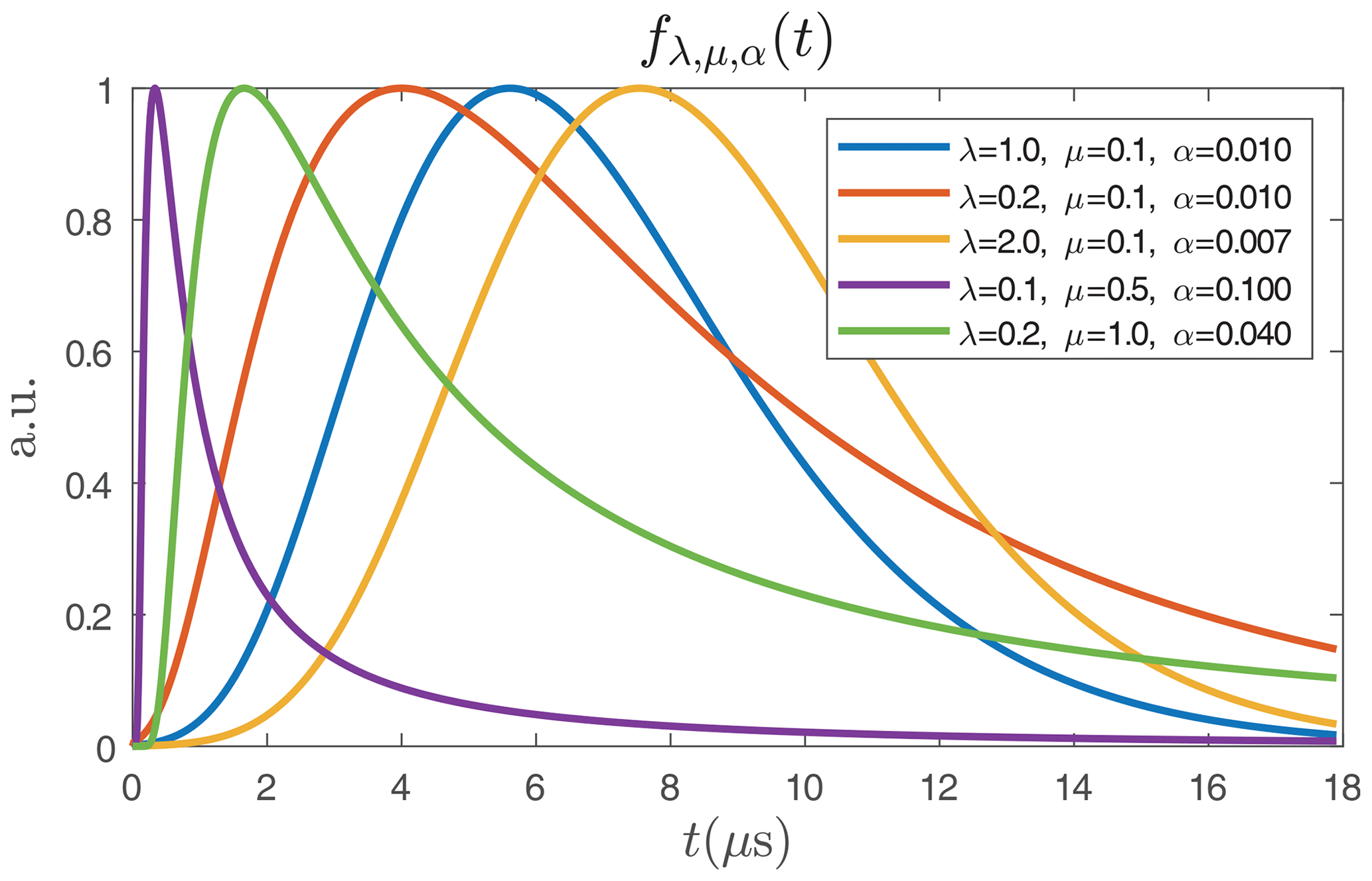
Figure 2Five examples of the probability density function of the inverse-Gaussian law which covers all shapes of the SAWR signal envelope.
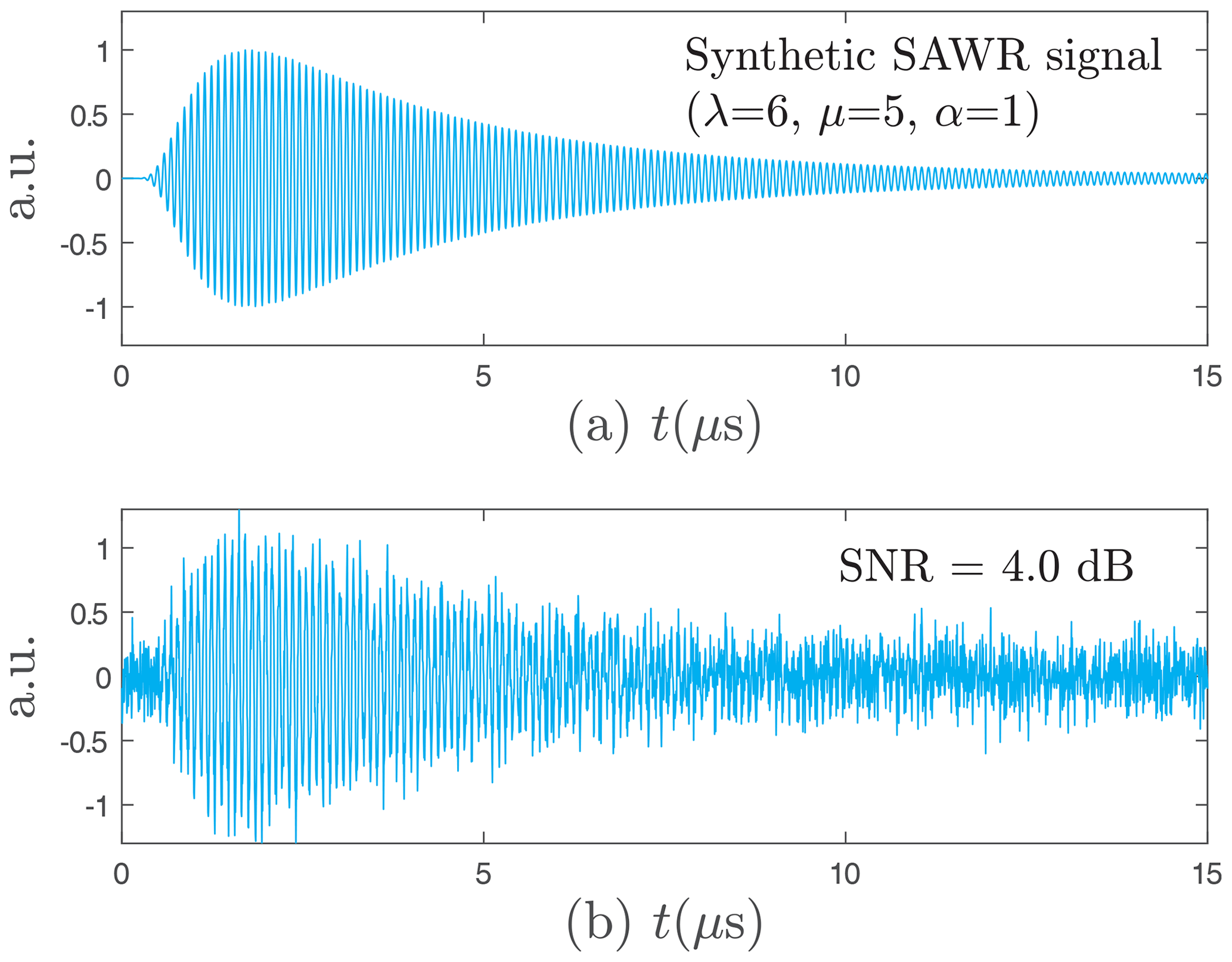
Figure 3The synthetic SAWR signal used for finding the best wavelet, with λ=6, μ=5, α=1, Fs=0.2 GHz, F=10.7 MHz and N=212 samples and T0=15 µs, (a) without noise and (b) with SNR =4 dB.
This modelling allows the identification of an experimental SAWR signal and roughly estimates its signal-to-noise ratio (SNR). Since the frequency range of the SAWR sensor is always known and since the signal contains a single main frequency, we can apply a low-pass filter with a cut-off frequency close to the resonance frequency F. Thus, by a local maximum detection on this filtered signal sf(t) and a cubic spline interpolation, we obtain the experimental signal envelope e(t). Finally, by using a least-squares algorithm, the different parameters λ, μ, and α of can be calculated, which leads to the model of the SAWR signal s(t) and an estimation of the SNR. This is depicted in Fig. 4.
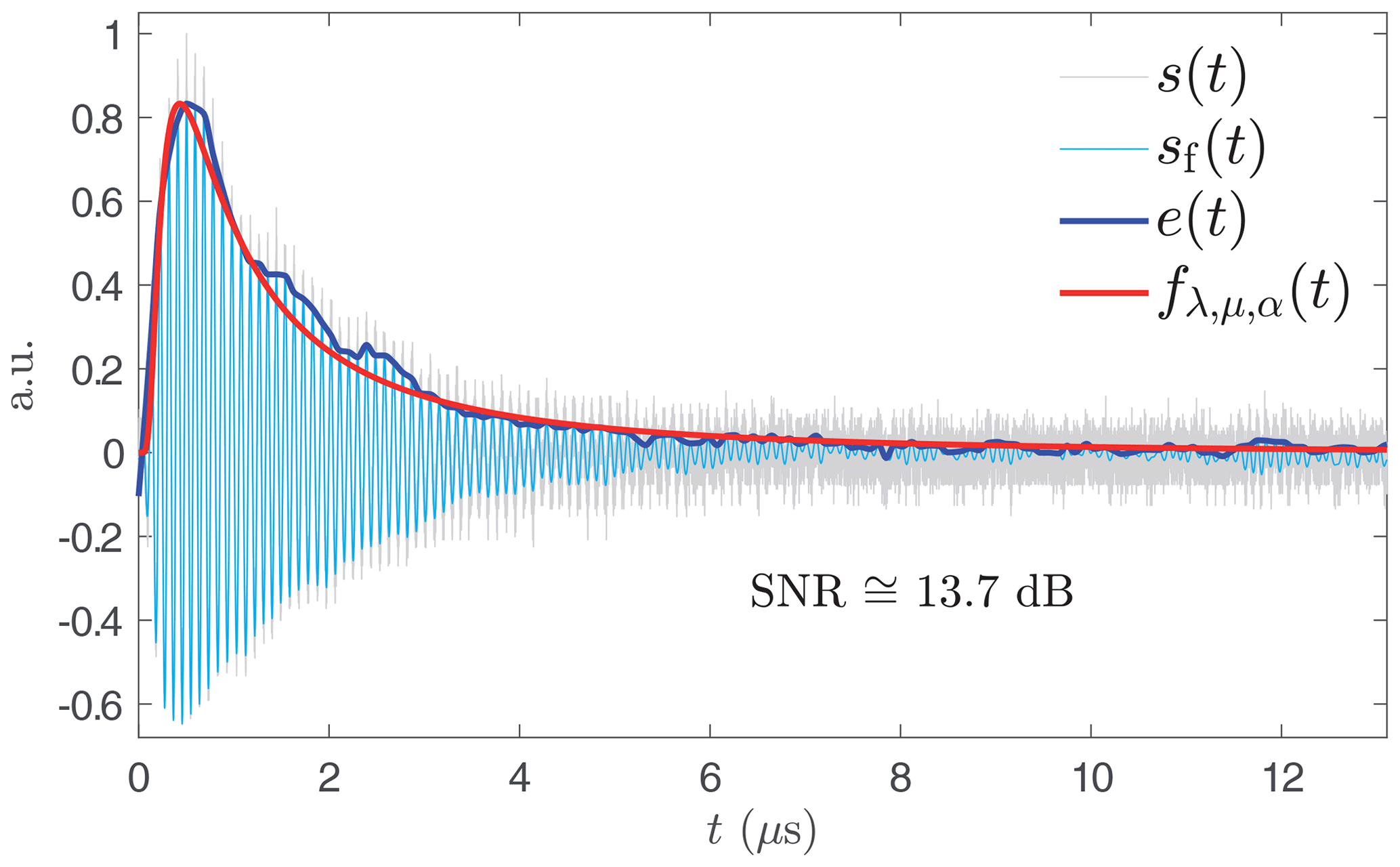
Figure 4Experimental SAWR signal (Fs=5 GHz, F=10.6 MHz, N=62 900 samples and T0=12.58 µs), modelled by the probability density function of an inverse-Gaussian law with λ=0.1, μ=0.2, and α=0.07. Estimated SNR =6.8 dB.
2.2 Wavelet choice
This modelling also the allows performance of a study concerning the best wavelet choice. If the EMD method offers no choice for the analysis functions, this is not the case for the wavelet transform. Indeed, there are many wavelet families, and it is necessary to select the best fit for the intended application. We do not neglect this rule, and hence we built a synthetic SAWR signal with the previous modelling to which we added a Gaussian white noise.
By varying the standard deviation of the noise, we generated 21 noisy signals with 4096 samples covering several reference signal-to-noise ratios (SNRRef) ranging from 0 to 20 dB (Fig. 3b). In order to obtain the best wavelet, we denoised each signal with 24 wavelets and computed the new SNR thereafter. The results are depicted in Fig. 5. Some wavelets stand out, i.e. Beylkin, Coiflet-5, Daubechies-20, Symmlet-10, and Vaidyanathan, for which a focus is given in Table 1. By minimizing the standard deviation, the one with the best average SNR is the Daubechies-20 wavelet, which was used for the wavelet-based method. The good results of this wavelet are directly related to its morphology, which agrees with that of the SAWR signal as shown in Fig. 6.

Figure 5SNR computation after denoising for 24 wavelets according to a reference SNR range (SNRRef) computed before denoising.
Table 1A focus on Fig. 5 for the best wavelets. SNR values computed after denoising.
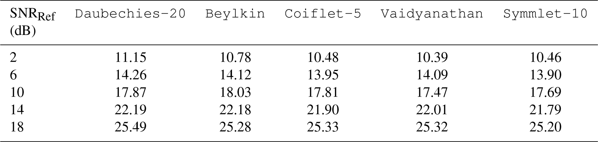
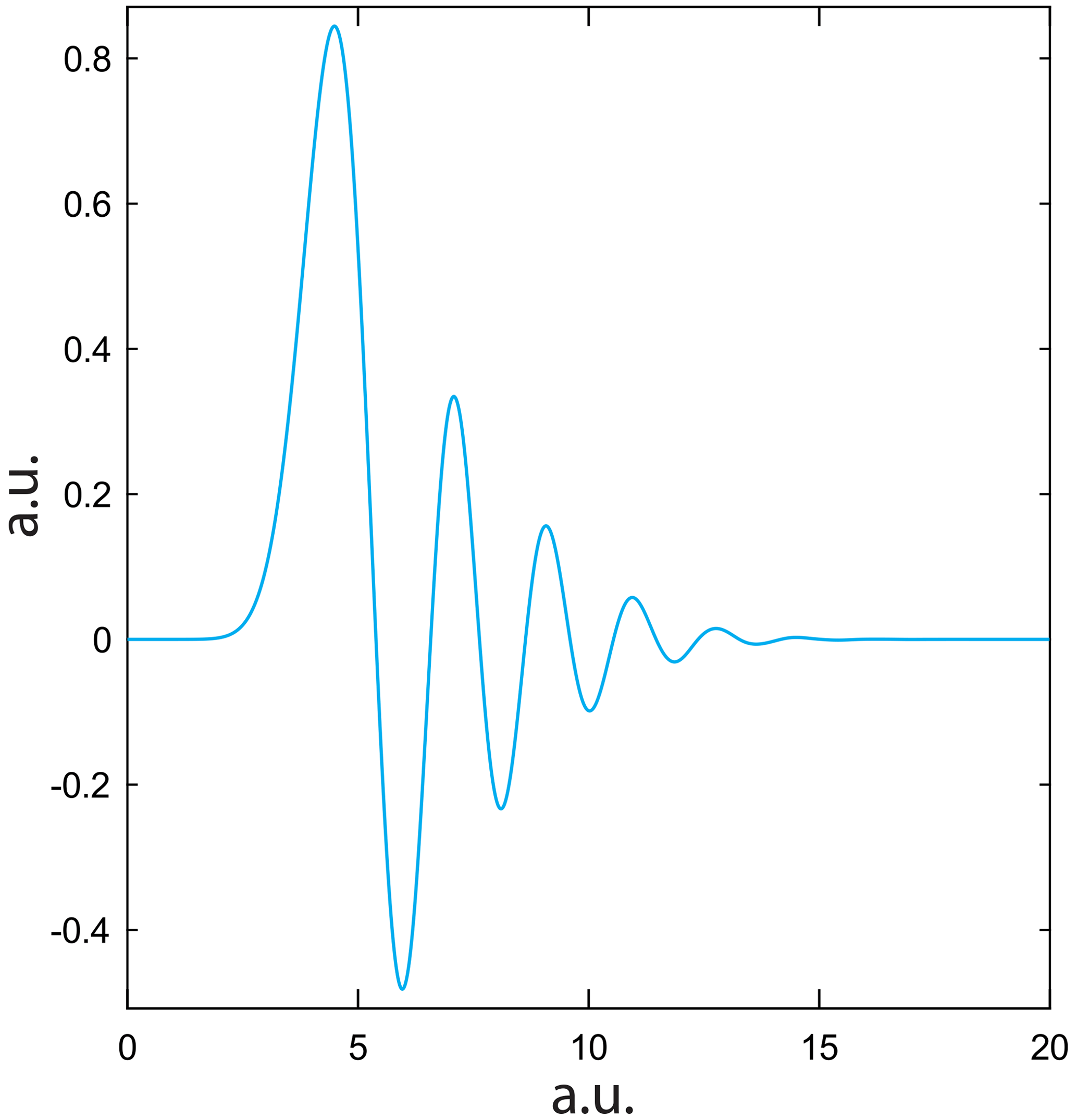
Figure 6Morphological behaviour of the Daubechies-20 wavelet (scaling function) chosen for the study.
2.3 Spectral and time-based methods
We implement spectral and temporal approaches which are particularly well suited to this work because the coherent signal contains only one main frequency. For the first one, an FFT is performed on the whole signal without any prior processing because this method is very robust to noise. The resonance frequency is obtained by finding the maximum modulus frequency. Figure 7 depicts this way.
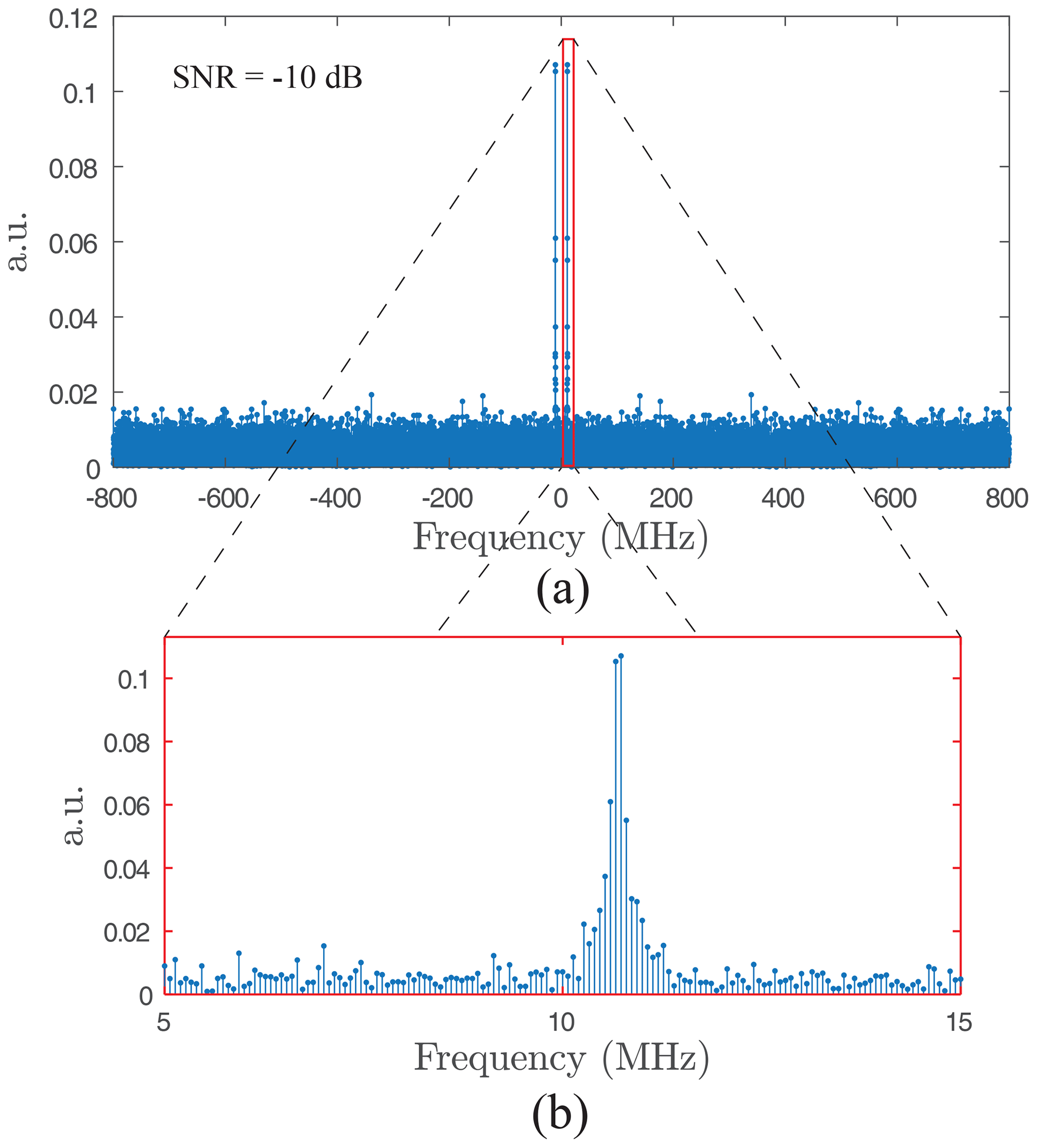
Figure 7Resonance frequency estimation with an FFT performed on the whole signal (Fs=1.6 GHz, SNR dB): (a) full bandwidth , and (b) zoom around the maximum modulus spectrum.
Unlike Fourier, which is robust to noise, a very important step of denoising must be performed for the time-based methods. To accomplish this, two common techniques are implemented and compared: wavelets and EMD. In particular, we implement the Antoniadis (Antoniadis et al., 2001) and Kopsinis (Kopsinis and McLaughlin, 2009) methods, respectively. In both cases, the default authors' settings were chosen. These two denoising techniques are very efficient, as depicted in Fig. 8 (the SNR gets better from 10 to 23 dB). The denoised signal allows a maximum detection procedure to be applied as described in Rischette et al. (2013). Finally, the researched frequency is obtained by computing the inverse of the average of all periods computed between each maximum.
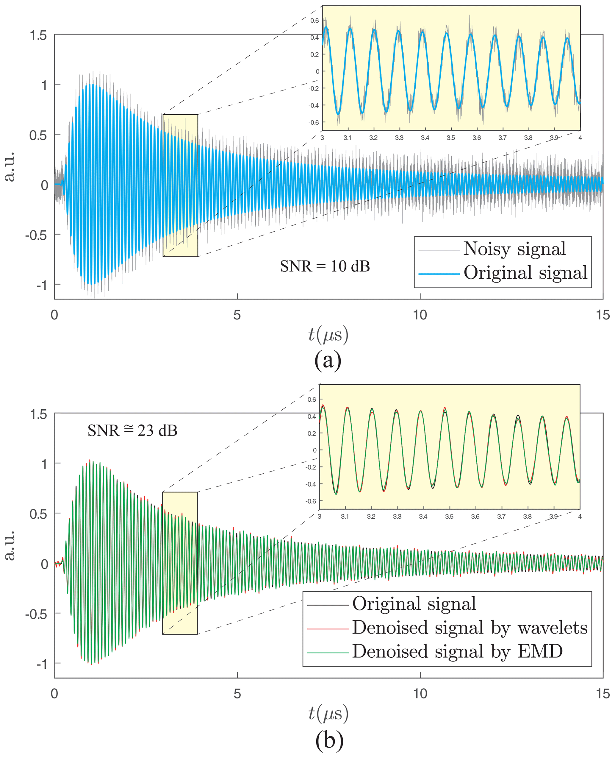
Figure 8Result of denoising techniques: (a) original and noisy synthetical signals with SNR =10 dB and (b) denoised signal by the wavelet and EMD methods (SNR =23 dB). The zoomed figures show that these two techniques are equivalent to a high-quality result since all three curves are almost superposed.
The time domain offers the advantage of choosing the portion of the signal for computation (a variable number of periods) without having a major impact on the precision. The resonance frequency will thereafter be the average of the different periods considered. The signal portion used for this calculation depends directly on the denoising quality and therefore on the SNR. As the SNR reduces, the more necessary it will be for a higher number of periods to be taken. On the other hand, if the SNR is high enough (greater than 5 dB), fewer than 10 periods will be sufficient to obtain a similar precision to the entire signal. In the case of Fourier, the search for minimum uncertainty imposes the consideration of FFT on the totality of the signal, as described in the following section.
3.1 Synthetic signals
SAWR signals s(t) were generated as described above with the parameters of Fig. 3 and for M=100 frequencies close to a usual intermediate frequency at F=10.7 MHz and for Q SNR values (Q=21 and dB) with N=8192 (213) samples, a sampling rate of Fs=1.6 GHz and a time duration T0=5.12 µs. These frequencies are represented in red in Fig. 9. The colour was chosen in order to avoid the masking of some represented figures. Also generated for each of the M frequencies are P=100 versions ηi(t) of the noised signal by an additive Gaussian white noise 𝒩(0,σh) with and Ps: the signal power of s(t) is
with , and .
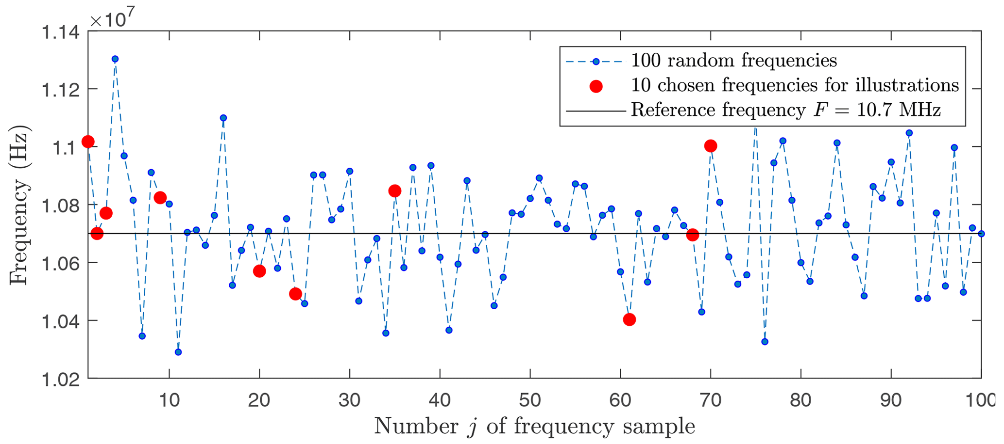
Figure 9Randomly computed frequencies , and M=100, with a Gaussian law 𝒩(m,σ), m=10.7 MHz, and σ=200 kHz.
3.1.1 Measurement accuracy
Figures 10 and 11 present a comparison of the relative error between wavelets and Fourier and between EMD and Fourier, respectively.
First, by observing both figures, through the yellow plans, we can see the invariability of the measurement by Fourier, regardless of the signal-to-noise ratio and the averaging rank of the noisy versions. As we might expect, we also see a progressive regularity of both 3D curves for wavelets and EMD as the number of averaged signals increases. In contrast, this regularity sets in much more quickly for EMD than wavelets. Regarding the wavelet or Fourier comparison, a dividing line appears at 0 dB and ends at −4 dB. It embodies the superiority of wavelets for signal-to-noise ratio values greater than this line (SNR dB). Concerning the EMD or Fourier comparison, the lesson is obvious: EMD is always superior to Fourier regardless of the signal-to-noise ratio, even in a single version of the noisy signal.
Figure 12 compares wavelets and EMD by displaying the positive value of the gap of the relative error. It is quite clear that the EMD provides more accurate results for SNR >10 dB. On the other hand, as soon as the SNR ⩽10 dB, the wavelets gain an advantage regardless of the number of averaged signals. In terms of the measured values, the Fourier error reached 0.52 %, i.e. 55.64 kHz for F=10.7 MHz against 0.013 % for the EMD and 0.011 % for the wavelets, or 1.39 and 0.97 kHz, respectively.
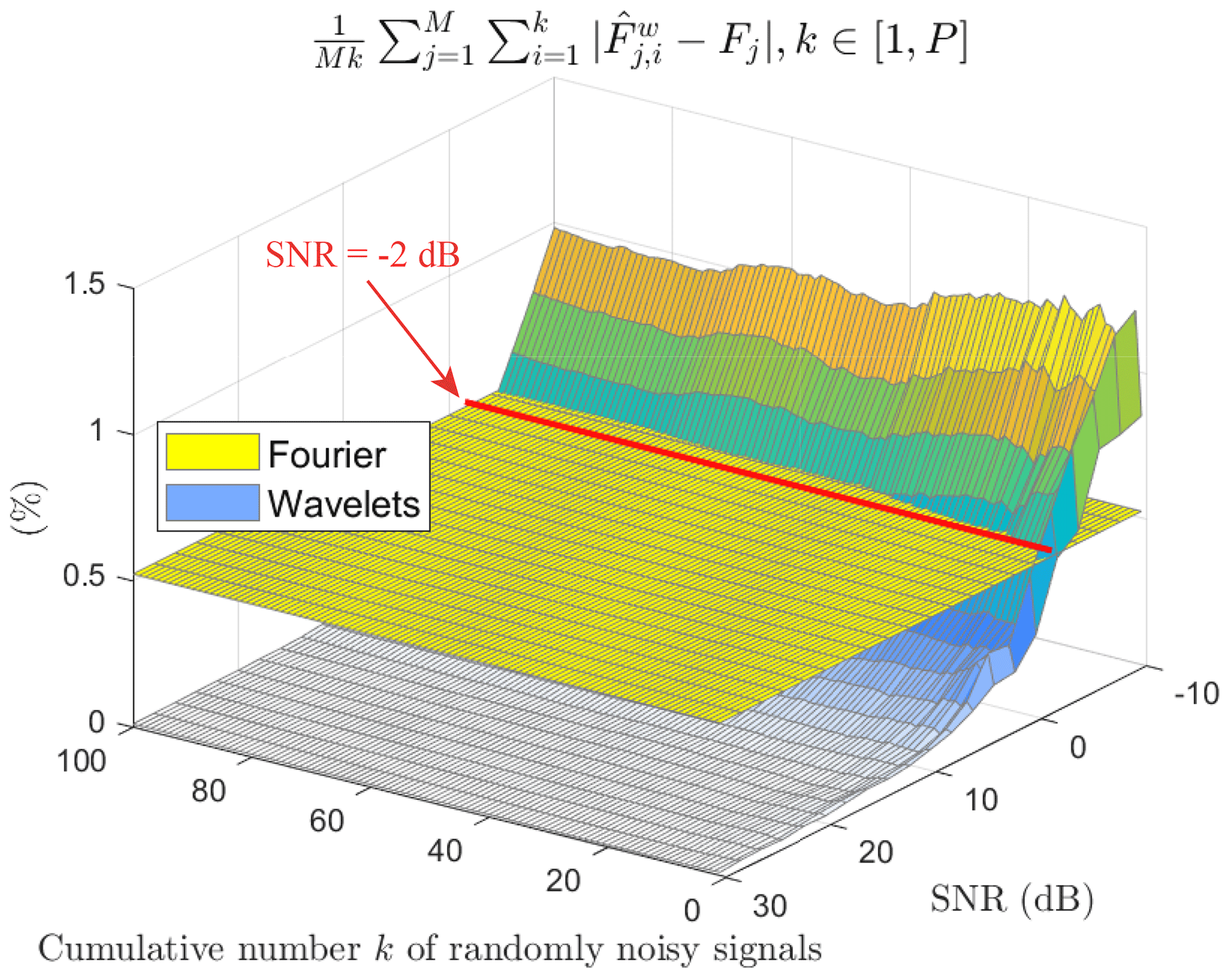
Figure 10Relative error for wavelets and Fourier between all the averaged estimated frequencies ) and the reference frequencies Fj versus SNR values and versus the progressive average of randomly noisy signals.
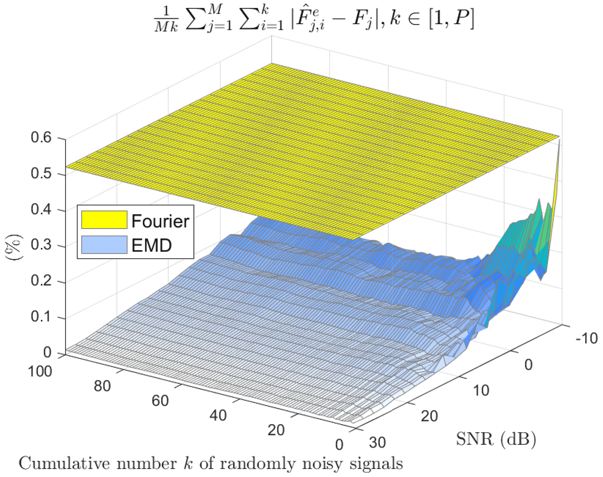
Figure 11Relative error for EMD and Fourier between all the averaged estimated frequencies ) and the reference frequencies Fj versus SNR values and versus the progressive average of randomly noisy signals.
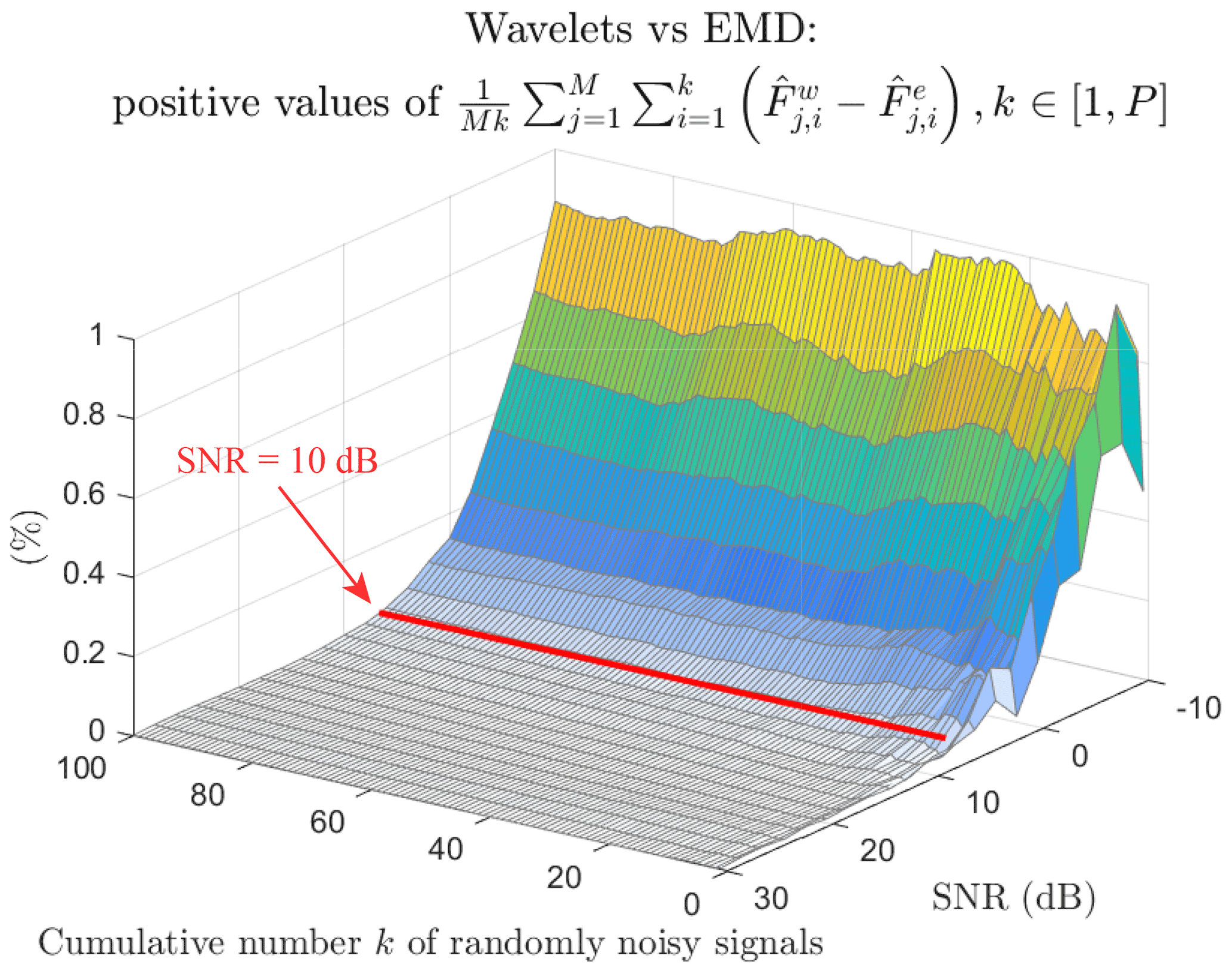
Figure 12Positive values of the relative error between all the wavelet averaged estimated frequencies ) and all the EMD averaged estimated frequencies versus SNR values and versus the progressive average of randomly noisy signals.
Another way of observing the behaviour of the error according to the SNR is proposed in Fig. 13 for each method: (a) Fourier, (b) wavelets, and (c) EMD. For the purpose of readability, in Fig. 9, only the results of frequencies chosen in red are displayed. Each curve corresponds to a studied frequency for a method and takes into account all the averaged versions of the signal (P=100).
For Fourier (Fig. 13a), the error is variable from one frequency to another but remains constant regardless of the SNR.
For wavelets (Fig. 13b), the behaviour of the error is more chaotic, reaching up to 15 dB. It then becomes stable and reaches values much better than those of Fourier.
For EMD (Fig. 13c), the evolution of the error is also variable, but its amplitudes are much smaller than those of Fourier and wavelets. As for the wavelets, the stability of the error is obtained above 15 dB.
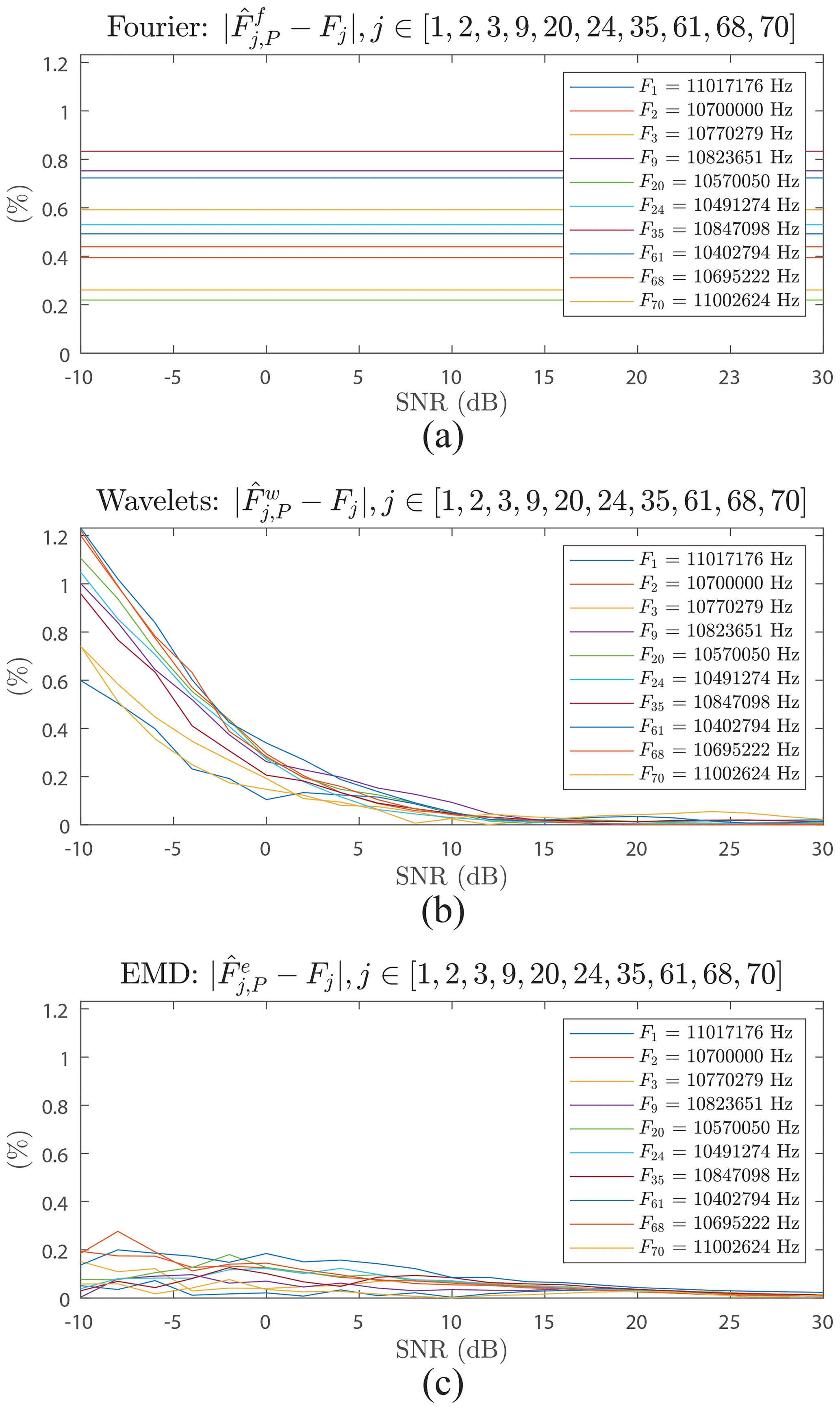
Figure 13Error between the estimated and reference frequencies versus SNR for (a) Fourier, (b) wavelets, and (c) EMD.
Figure 14 shows the relative average error between all the averaged estimated frequencies and for P=100) and the reference frequencies Fj for each SNR value as Fourier, EMD, and wavelet approaches. Regardless of the SNR level, the values obtained by the FFT are always the same. This is not a surprising result since the FFT is a robust tool against noise. On the other hand, this constancy in the results proves the inability of the FFT to discriminate between frequencies close to each other (less than 50 kHz, apart from F=10.7 MHz). For the full studied SNR range, EMD and wavelets are better than Fourier except for dB, where wavelets are no longer competitive. Figure 14 allows us to conclude that, in the range 8 dB, the EMD method is most efficient, while in the range dB it is preferable to use wavelets, with a precision of up to 47 times better than Fourier.
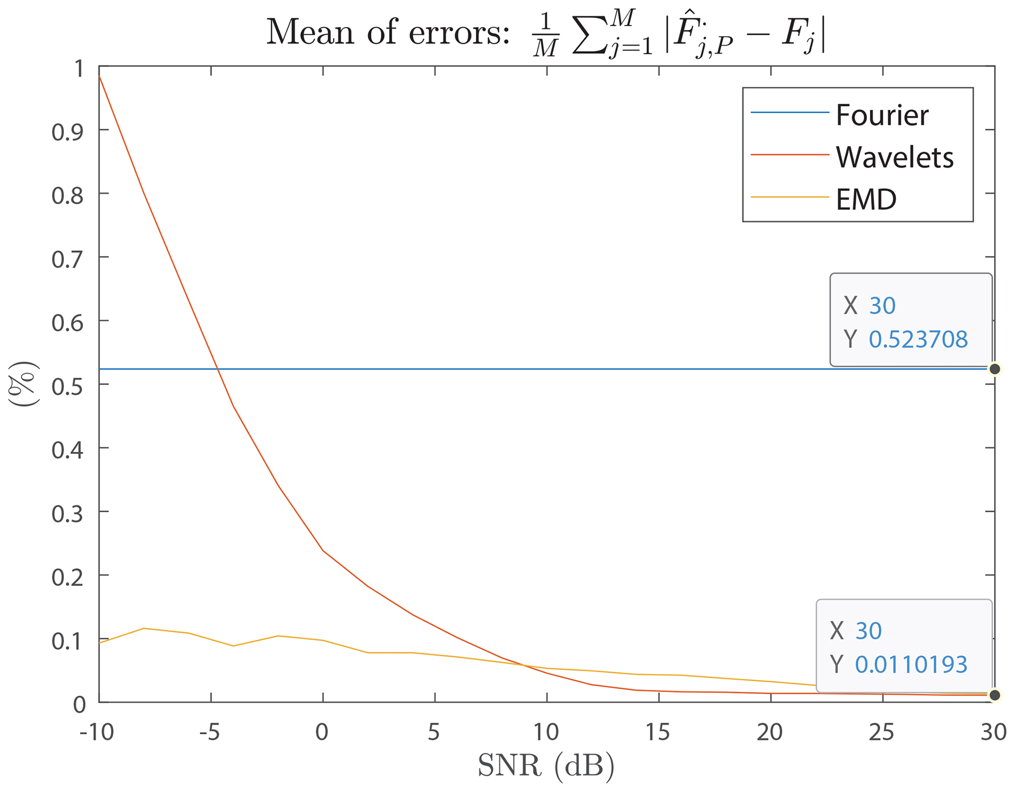
Figure 14Mean of errors between estimated and reference frequencies versus SNR for Fourier, EMD, and wavelet approaches.
3.1.2 Measurement uncertainty
In addition to accuracy, it is important to consider the uncertainty of the measurement.
For the FFT approach, uncertainty is related to the spectral resolution ΔFf, which only depends on the time duration T0 with
Therefore, FFT uncertainty depends only on duration and not on the number of samples or the signal frequency. This is the reason why the entire duration of the signal must be considered to obtain the smallest uncertainty.
Unlike Fourier, the uncertainty ΔFt for both time-based methods depends on the signal frequency and the sampling period Fs, i.e. the difference between two consecutive samples. The relation is given by
and finally
Figure 15 depicts uncertainties ΔFf and ΔFt of the estimated frequency according to the reference frequency F and the sampling frequency Fs. The results are enlightening as soon as Fs>500 MHz, which is the intersection between ΔFf and ΔFt. Even if the wavelets or EMD uncertainty are slightly degraded as F increases, they are significantly lower than the Fourier uncertainty in the ratios of 3, 18, and 36 for Fs=1.6, 10, and 20 GHz, respectively. The Fourier uncertainty plan is slightly tilted due to its constant value expressed in a percentage.
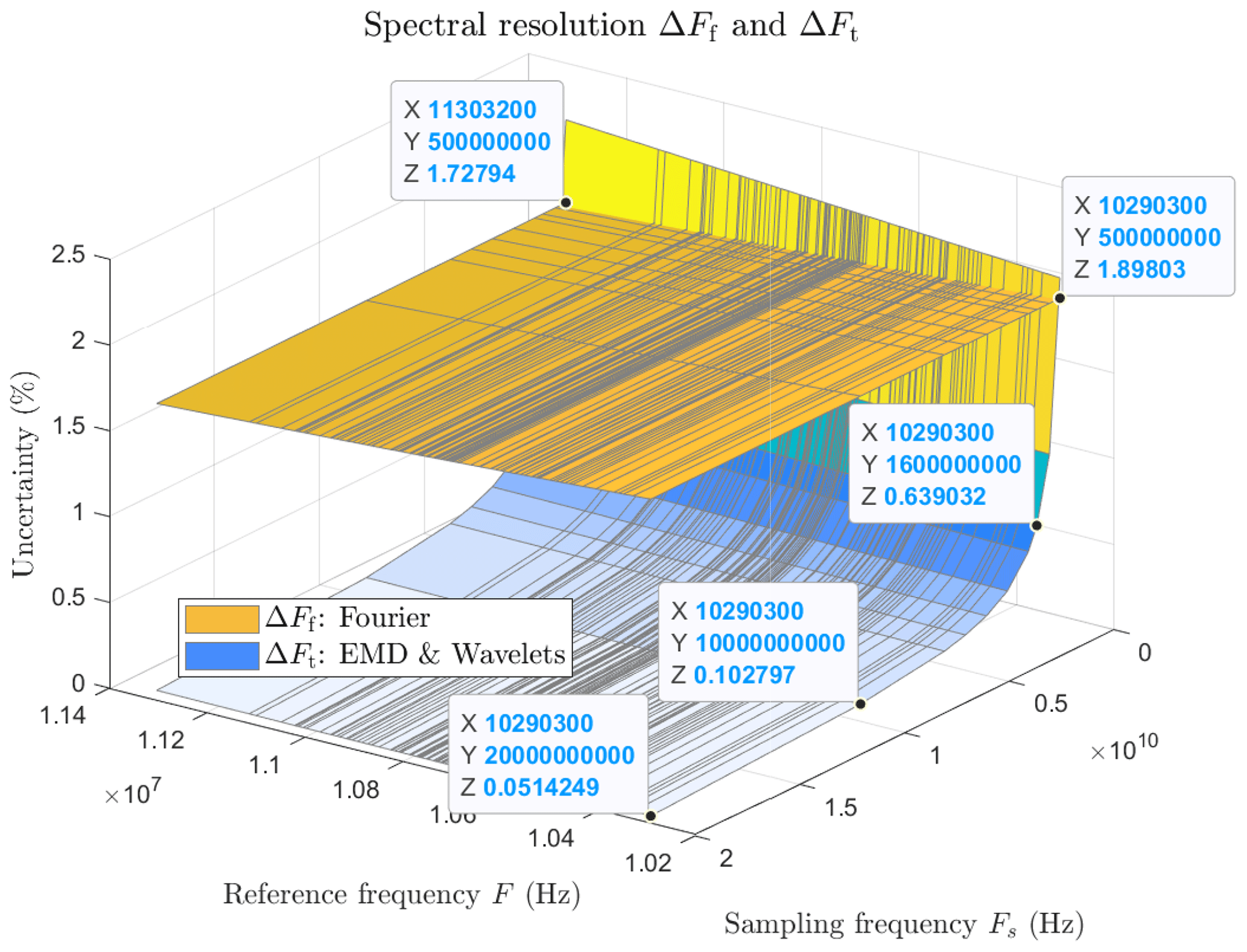
Figure 15Uncertainties ΔFf (Fourier) and ΔFt (W/EMD) of the estimated frequency versus the reference frequency and the sampling frequency.
3.2 Experimental signals
Figure 16 shows the block diagram of the experimental setup while performing signal acquisition using a radiofrequency (RF) module. The signals are generated by a RF generator. They are then transmitted to the SAWR via an antenna and a RF switch. Their initial central frequency is Fn=868 MHz, and the responses of the SAWR are translated at F=10.7 MHz using a RF down-converter.
Tables 2 and 3 show the results for the three signals with different numbers of samples, sampling rates, and a constant time duration T0=13.1 µs. The superiority of the time-based methods is confirmed in terms of uncertainty.
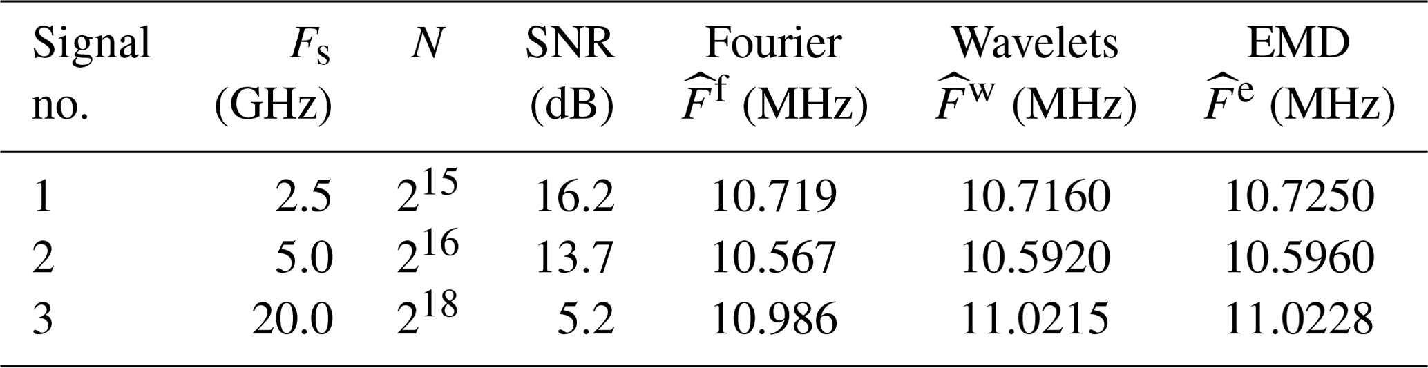
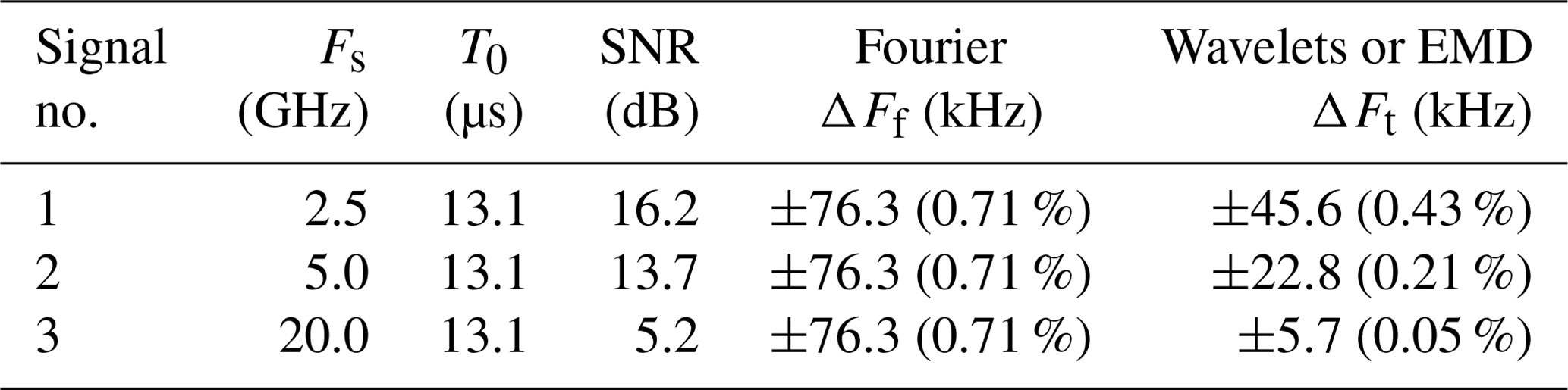
Signal no. 1 (Fig. 17) is characterized by a Gaussian envelope, Fs=2.5 GHz, N=32 768 (215), and an estimated SNR =16.2 dB. The estimated frequencies are close in all three cases (Table 2), with an improved wavelet or EMD spectral resolution of 40 % with respect to Fourier (Table 3). Taking into account the SNR and with regard to Fig. 14, the right value is probably given by the wavelet method with .
Signal no. 2 (Fig. 18) is characterized by Fs=5 GHz, N=65 536 (216) and an estimated SNR =13.7 dB. The frequency difference between the time-based and Fourier approaches is about 30 kHz, while between the two time-based methods this difference is only 4 kHz (Table 2), which confirms the results of Fig. 14. Furthermore, the uncertainty of wavelets or EMD is clearly better since its improvement reaches a ratio of 3 in comparison with Fourier (Table 3). For the same reasons as above, the right frequency seems to be given by the wavelet method with .
Signal no. 3 (Fig. 19) is much noisier than the previous two and is characterized by Fs=20 GHz, N=262 144 (218) and an estimated SNR =5.2 dB. The gap between Fourier and wavelets or EMD is about 40 kHz against 1.3 kHz between the wavelets and EMD (Table 2). SNR =5.2 dB corresponds to a range for which the measurement accuracy by wavelets is better than EMD (Fig. 14). The uncertainty value decreases to 5.7 kHz against 76.3 kHz for Fourier, which represents 0.05 % of the central frequency (Table 3). The true value is probably kHz.
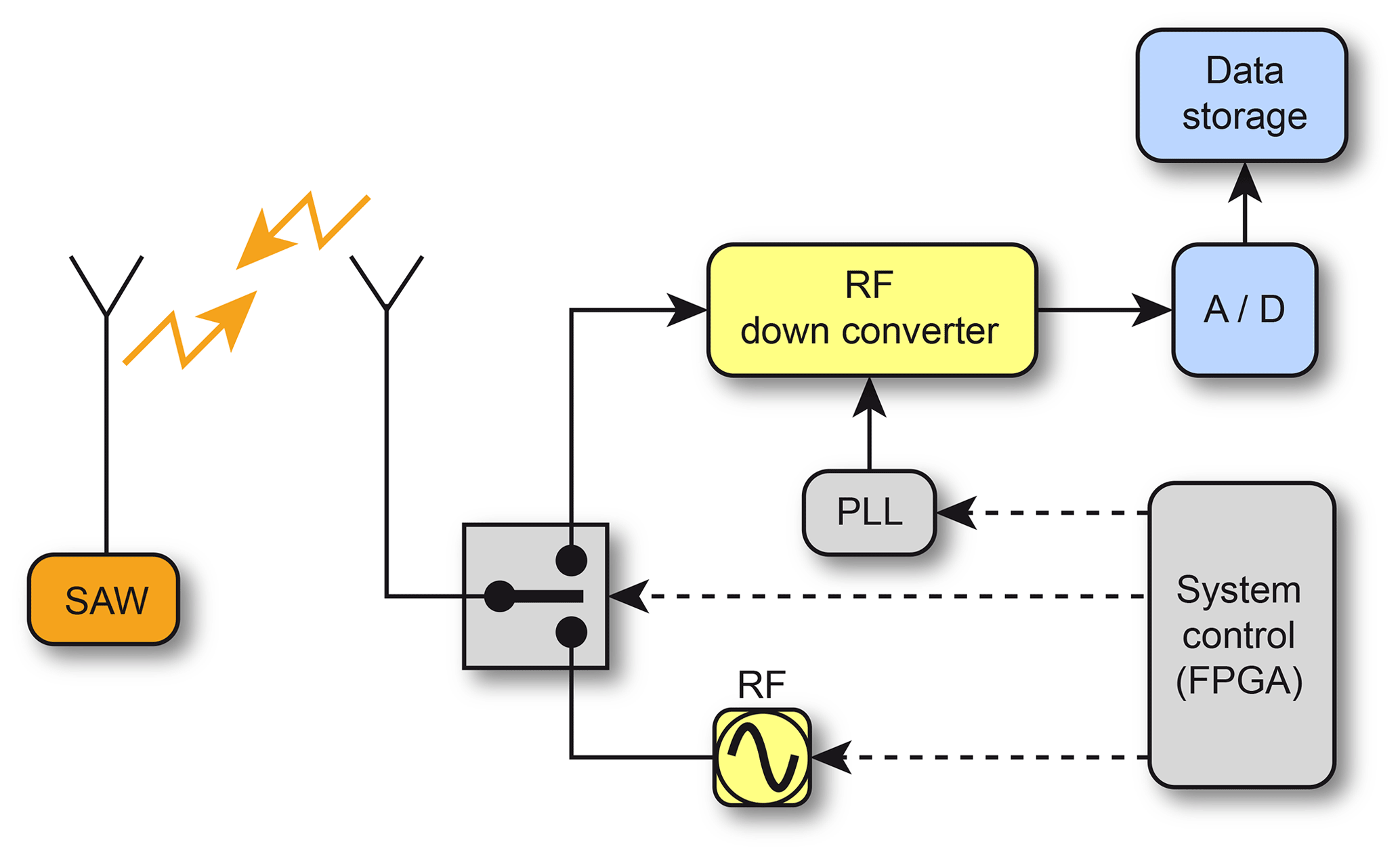
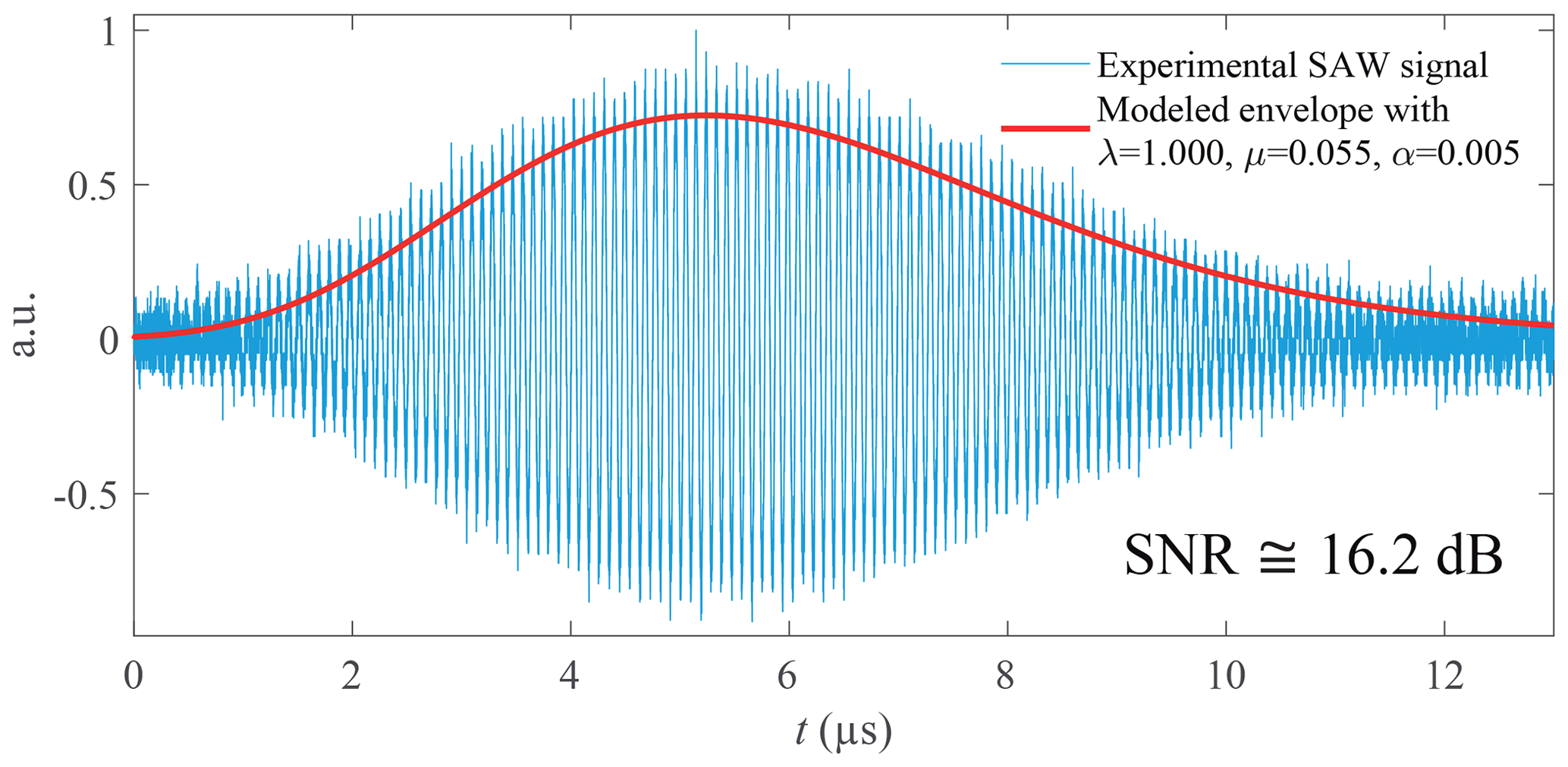
Figure 17Experimental SAWR signal no. 1 with low-pass filtering at 20 MHz (Fs=2.5 GHz, N=215 samples, and T0=13.1 µs).
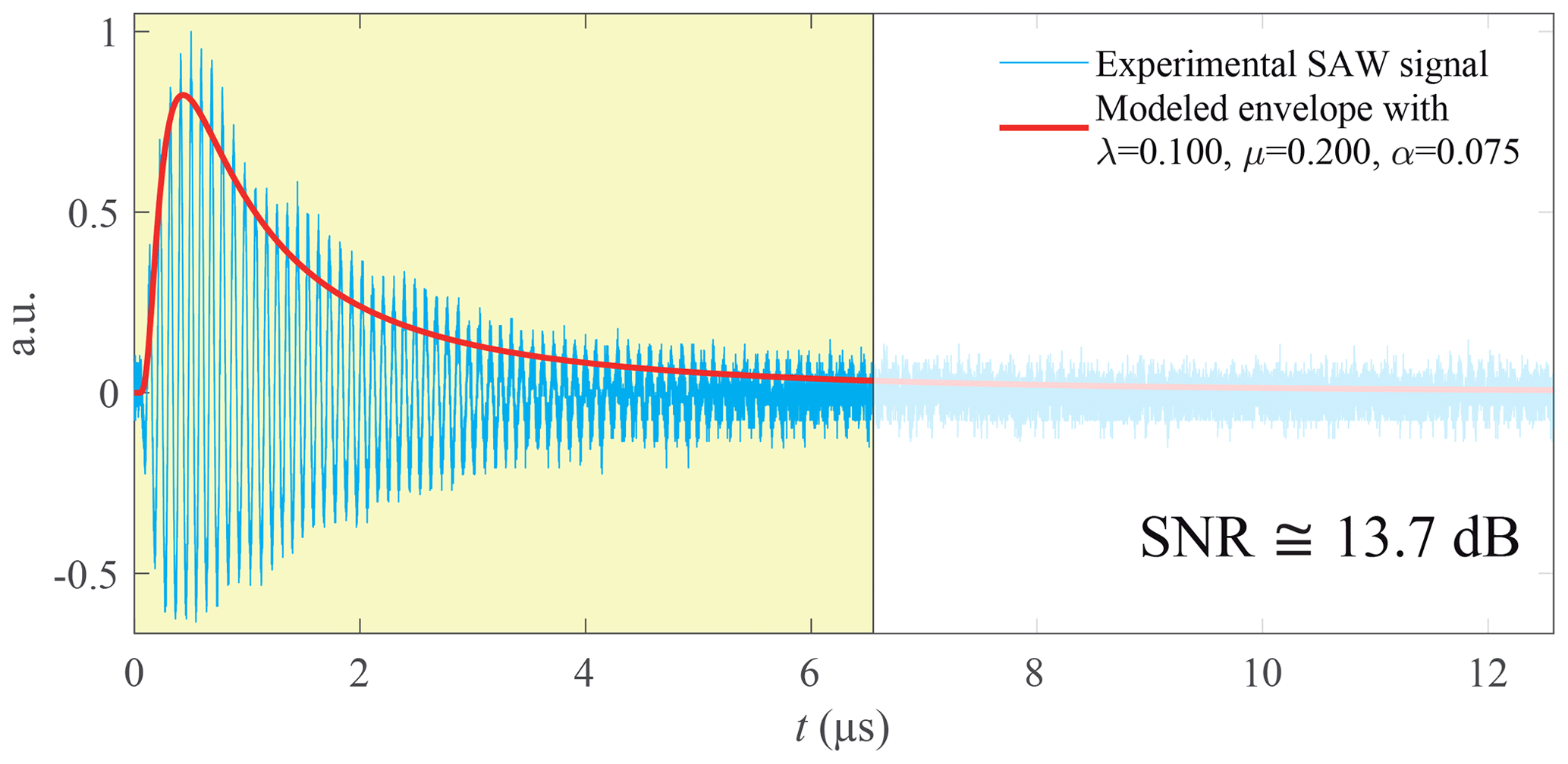
Figure 18Experimental SAWR signal no. 2 with low-pass filtering at 20 MHz and lag (yellow in the colour version) used for the time-based methods (Fs=5 GHz, N=216 samples, T0=13.1 µs, and lag =6.55 µs used for the time-based methods).
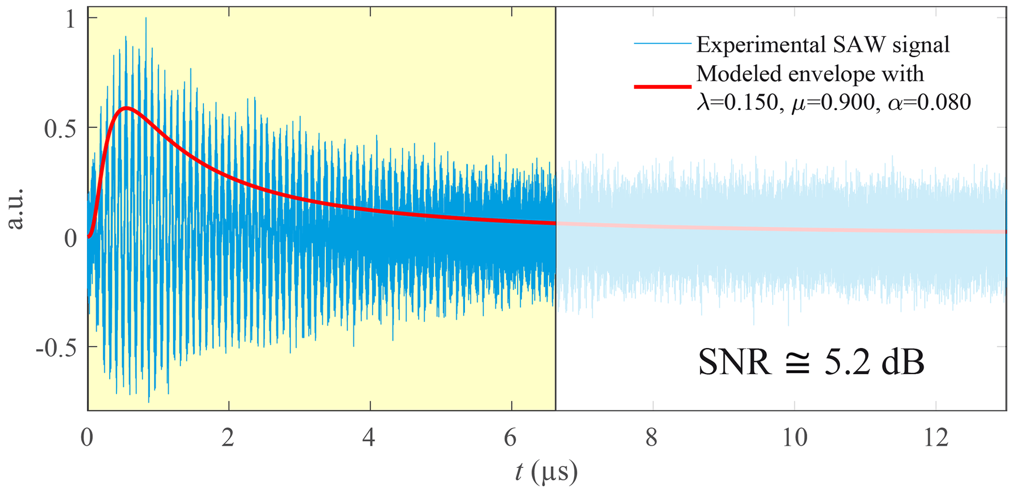
Figure 19Experimental SAWR signal no.3 without filtering and lag (yellow in the colour version) used for the time-based methods (Fs=20 GHz, N=218 samples, T0=13.1 µs, and lag =6.55 µs used for the time-based methods).
3.3 The case of SAWR temperature sensors
In this subsection, we describe the impact of previously established frequency results on the temperature accuracy measured for this kind of sensor.
The frequency translation shown in Fig. 16 shifts the response of the sensor centred around Fn=868 MHz to a lower intermediate frequency F=10.7 MHz but maintains its spectral characteristics (amplitude, frequency width, etc.). Therefore, the results obtained at F=10.7 MHz are applicable to the industrial, scientific, and medical (ISM) bands in the ranges 433 MHz, 868 MHz, and 2.4 GHz.
Most SAWR temperature sensors are based on the piezoelectricity phenomenon. Whatever the material category (single crystal, film, or ceramic), the central frequency of this kind of SAWR sensor can be connected to the temperature through the TCF (temperature coefficient of frequency) by a linear approximation:
or by a quadratic approximation with this form:
We chose four SAWR temperature sensors from one of the frequency bands mentioned above. Two of them come from scientific articles and the other two from a manufacturer's documentation. Their references and central frequencies are respectively as follows:
-
Sensor 1 (SS433FB2), F1n=434.56 MHz (SAWComponents, 2013),
-
Sensor 2 (AlN-SAW), F2n=501.18 MHz (Wang et al., 2023),
-
Sensor 3, F3n=897.37 MHz (Liu et al., 2017),
-
Sensor 4 (SS2414BB2), F4n=2.41635 GHz (SAWComponents, 2014).
The considered elements characterize the TCF (Fig. 20a). These data establish with the desired level of precision the temperature–frequency relationship (Fig. 20b). We apply our frequency measurement method to the different sensors mentioned above. To compare the results for these sensors, we choose to calculate the TCF as
Equation (9) leads to the temperature–frequency relationship:
The results are depicted in Table 4. For a low-noise signal (SNR =30 dB, Fig. 10), the best frequency accuracy obtained by the wavelets is 0.97 kHz, which corresponds to a temperature accuracy of ±0.06 ∘C for a 433 MHz sensor and ±0.01 ∘C if the sensor is in the 2.4 GHz band.
Table 4Temperature precision according to the frequency measurement.
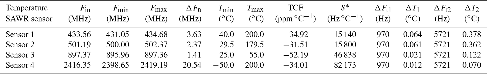
* Sensitivity.
For a strongly noisy signal (SNR =5 dB, Fig. 19), the best frequency accuracy is 5.7 kHz, which corresponds to a temperature accuracy between ±0.07 and ±0.38 ∘C according to the central frequency of the sensor.
Currently, the usual temperature accuracy is ±0.1 ∘C for a single measurement and reaches ±0.01 ∘C in the averaged multiple measurements. The results presented in this paper reach an accuracy of ±0.07 ∘C in one shot for the 2.4 GHz ISM band in a very noisy environment. The accuracy even reaches ±0.01 ∘C for a slightly noisy signal.
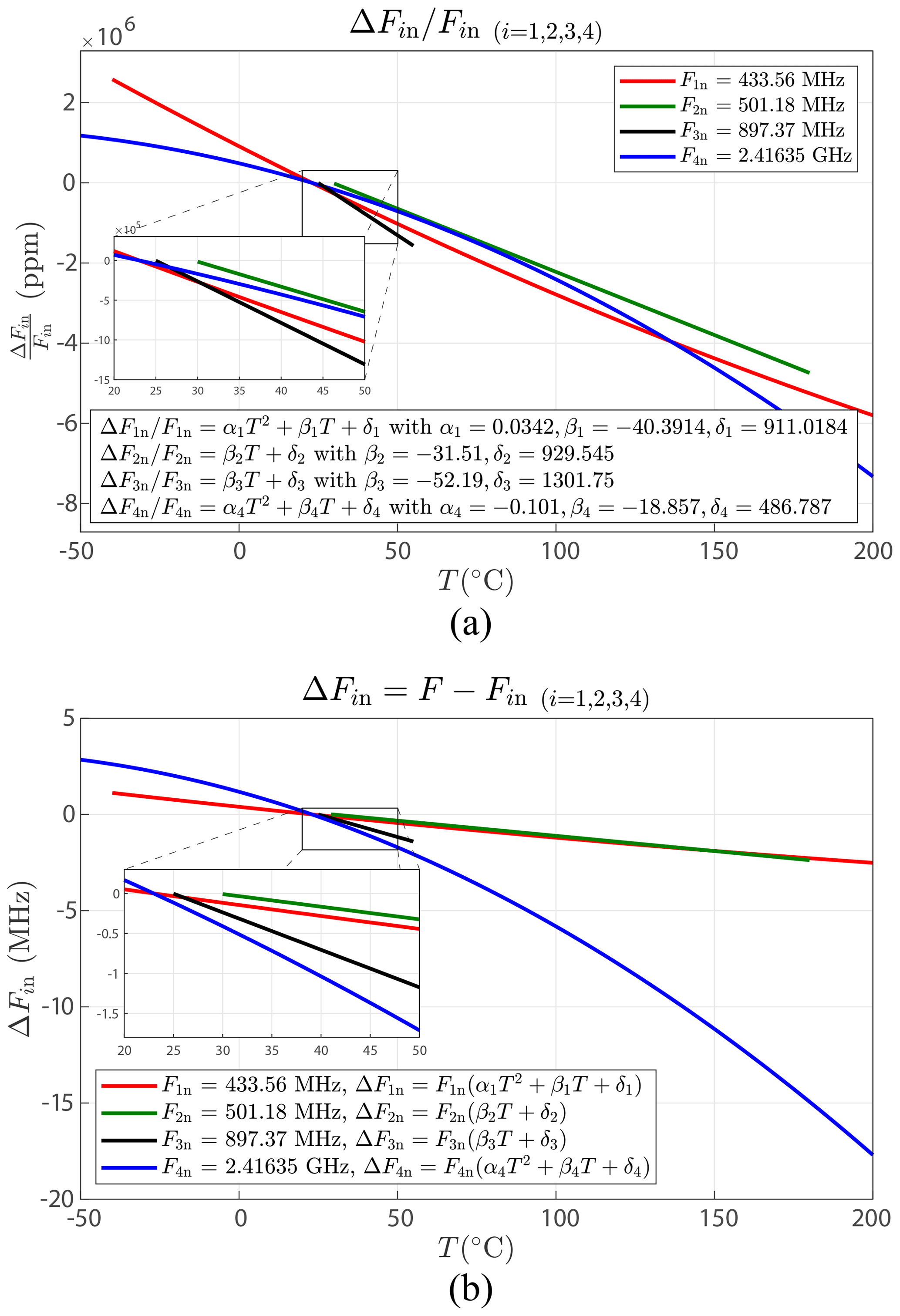
Figure 20Frequency behaviour according to the temperature ranges for different temperature SAWR sensors: (a) temperature coefficient of frequency and (b) frequency shift.
Measurement of resonance frequency variation is fundamental for all applications using a wireless SAWR sensor. We proposed a comparative study for the estimation of this frequency between the usually FFT spectral method and two time-based methods, the first using a wavelet approach and the second applying empirical mode decomposition (EMD). A model which describes the behaviour of SAWR signals and also allows the generation of synthetic signals was also proposed. This model was implemented to address the question of the wavelet choice as part of the first method, and it leads to the Daubechies-20 wavelet. Both time-based ways are compared as well as with the reference way: the Fourier transform. Synthetic and experimental signals are used to evaluate these three solutions. Results obtained by the time-based (wavelet and EMD) methods are distinctly better than those of the FFT. According to the different SNR values, the improvement in accuracy reaches a factor of 47 and, in uncertainty, a factor of 36. Finally, this study shows that the EMD method is better when the signal-to-noise ratio is less than 8 dB and the wavelet method is preferable when it is greater than 8 dB. Moreover, these frequency results have been applied to SAWR temperature sensors. The accuracy reaches up to ±0.01 ∘C in one shot. Future research could provide better accuracy and uncertainty by introducing up-sampling. A study of the number of periods according to desired precision and uncertainty could also be of interest to optimize the computation time.
Presented here is the theoretical background of the two main methods employed in this study: the continuous–discrete wavelet transform and the empirical mode decomposition.
A1 Wavelet transform
A1.1 Continuous wavelet transform (CWT)
The CWT is defined as
with a the scaling factor, b the translation parameter, ψ* the complex conjugate of ψ, and
The mother wavelet ψ checks the following properties:
-
A number of vanishing moments m characterizes the mother wavelet ψ such as
where is the scalar product.
In this case the wavelet analysis is blind to any polynomial of degree lower than m−1, and therefore this property is decisive in optimizing the detection of a singularity.
-
The wavelet transform also has the ability to reconstruct the signal s from the decomposition coefficients by
subject to
which is checked if the admissibility condition is respected,
or also that
with ψ∈L2(ℝ).
The wavelet transform is a powerful tool for the detection of singularities in a signal. By calculating the Hölder exponent (or Lipschitz) and using wavelet transform modulus maxima, it is possible to emphasize the properties of these singularities. Figure A1 depicts a continuous wavelet analysis of an example signal with the signal at the top, the wavelet coefficients in the middle, and local modulus maximum lines at the bottom.
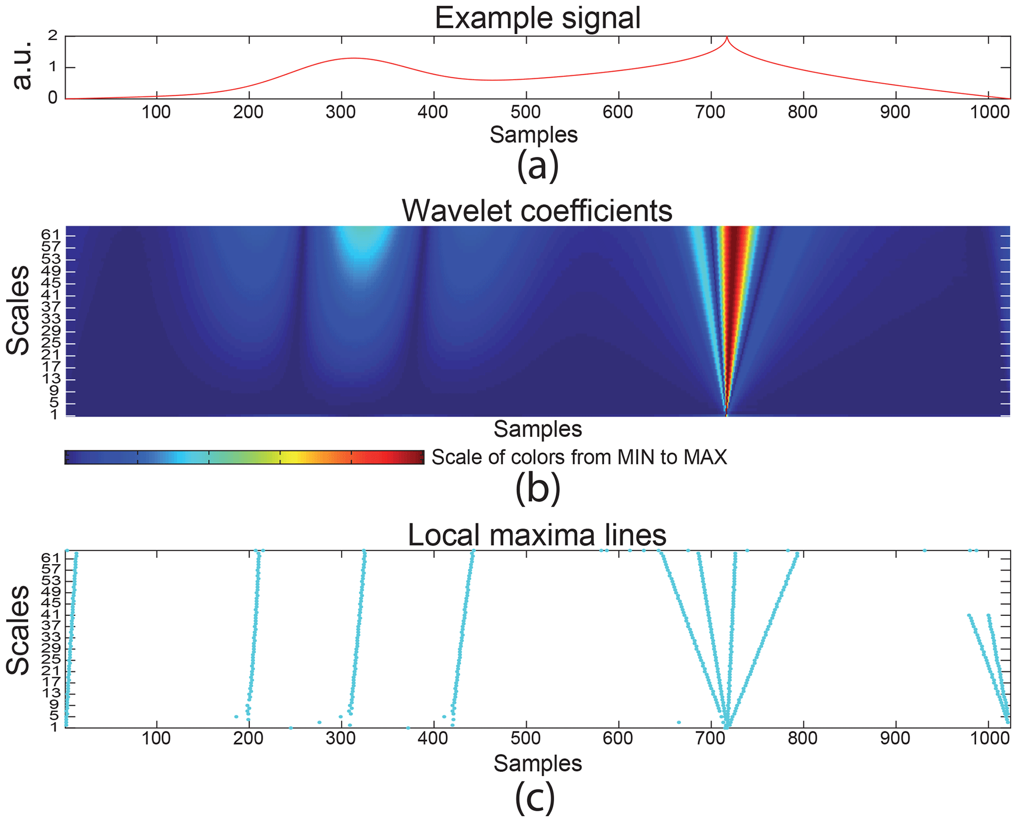
Figure A1Continuous wavelet analysis on a test signal with 1024 samples and a wavelet symlet 2: (a) the analysed signal, (b) wavelet coefficient scalogram, and (c) local modulus maxima lines.
Let and . The CWT can be written as
with .
For u0=2 and v0=1 this dyadic transform becomes the discrete wavelet transform given by
A1.2 Discrete wavelet transform (DWT)
Unlike the CWT, the DWT is defined by two functions: the scaling mother function φ and the wavelet mother function ψ (Chen et al., 2016; Mallat, 1989). Therefore, there are two bases that analyse the signal s. These are defined as
with j the scaling factor and n the translation parameter .
A link between this approach by the scale and wavelet functions and the filter theory was established in particular by Stéphane Mallat (Mallat, 1989) and led to the multi-resolution analysis (MRA). The MRA is based on two filters: the approximation filter h (low-pass) and the detail filter g (high-pass) for which the impulse responses are defined by
where .
The MRA is very well suited for denoising a signal since it naturally separates the signal into approximations and details at different scales.
This is depicted in Fig. A2. One can observe on the left the signal increasingly denoised through scales.
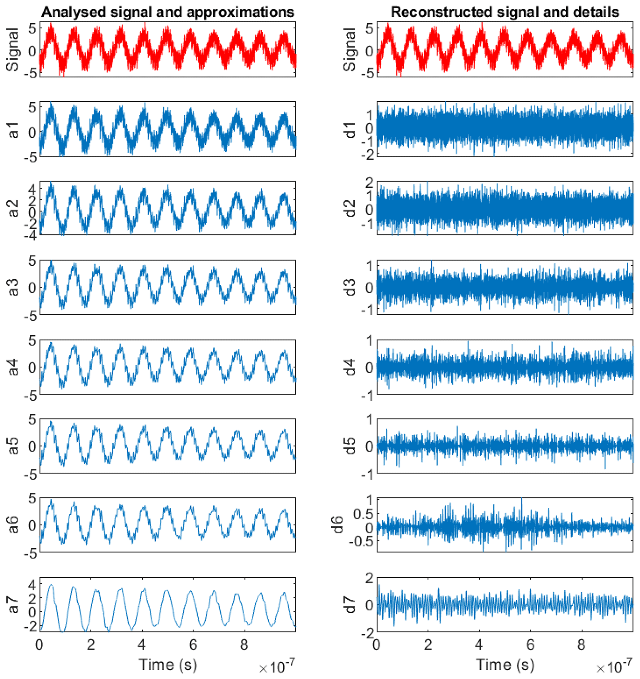
Figure A2Multi-resolution analysis of a zoomed experimental SAWR signal using a wavelet Symlet 4 with approximations on the left and details on the right.
A2 Empirical mode decomposition (EMD)
As wavelets, the EMD method analyses signals in scales. The difference between Fourier or wavelets and EMD is the analysing basis. The EMD is based on oscillating functions extracted from the signal itself (Keshtan and Khajavi, 2016; Huang et al., 1998). The oscillating functions are built algorithmically and iteratively by a subtraction between the mean envelope and the residual signal (Chen et al., 2018). This is the mean of the upper and lower envelopes, built from a cubic spline interpolation (Fig. A3). The oscillating functions obtained are so-called IMFs (intrinsic mode functions).
The EMD algorithm is detailed in Fig. A4. Its principle is based on two loops. The first one (Fig. A4 on the left) builds the current IMF from the signal bereft of its previous IMFs from which it gradually subtracts the mean envelopes. The second loop (Fig. A4 on the right) manages the extraction of the IMFs.
Thus, the signal s(t) is written as
with rn(t) the residue (three extrema maxima), imfi(t) the oscillating function at scale i, and .
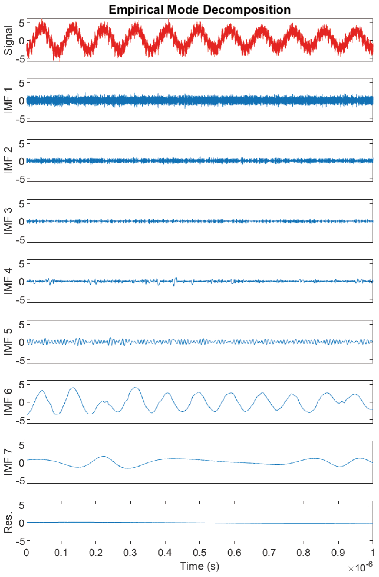
Like DWT, the EMD method analyses the signal into scales and is well suited for denoising. This is depicted in Fig. A5, which shows the progressive separation between low (high IMF number) and high (low IMF number) frequencies.
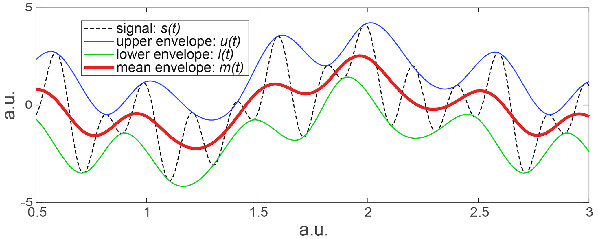
Figure A3Building of the upper, lower, and mean envelopes which are the key points of the iterative algorithm of an intrinsic mode function (IMF) calculation.
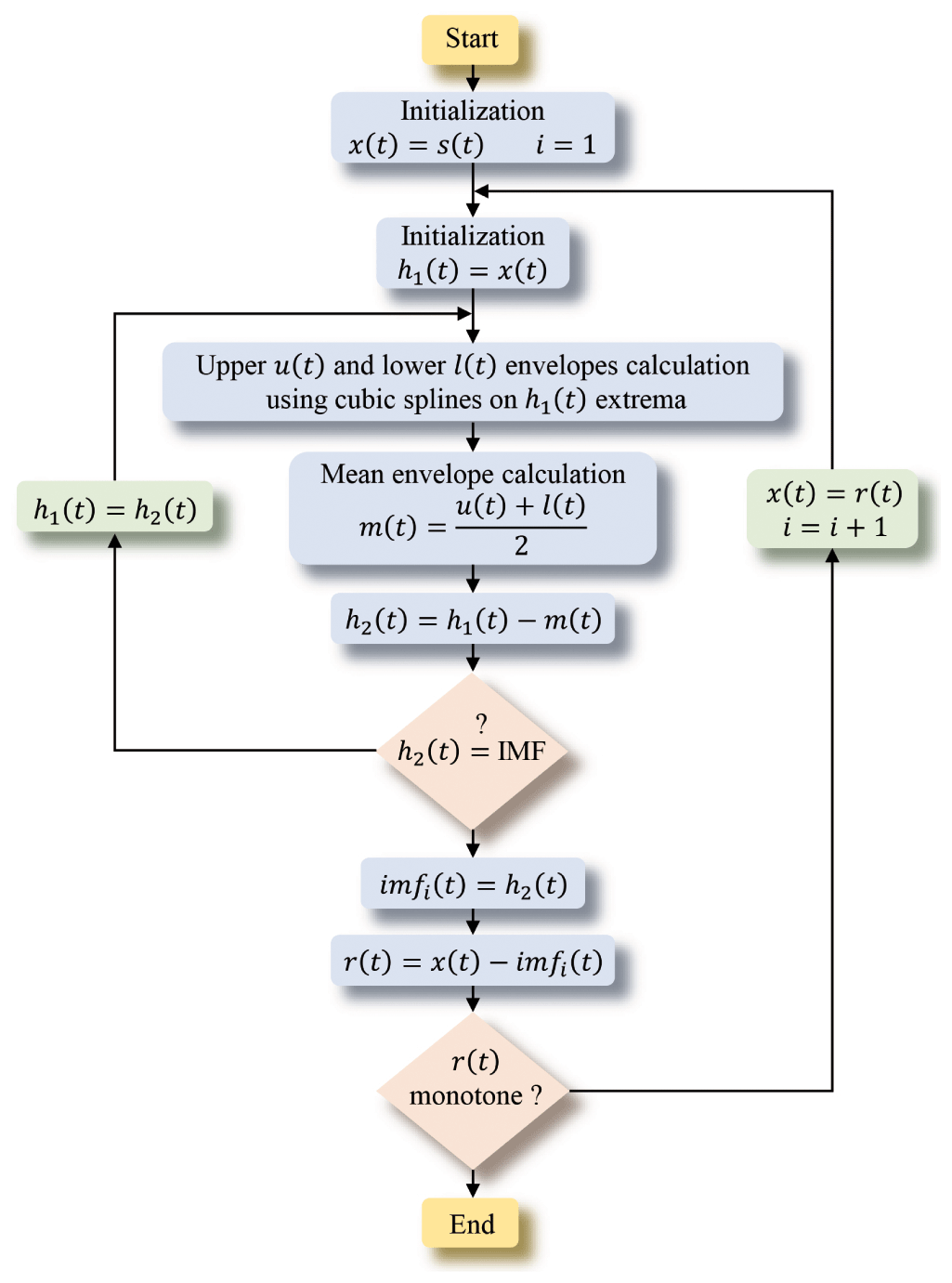
Figure A4EMD algorithm that gradually extracts all the intrinsic mode functions imfi(t) from the signal s(t).
| Fn | SAWR resonance frequency |
| F | Fn translated at 10.7 MHz |
| Estimated resonance frequency by Fourier | |
| Estimated resonance frequency by wavelet | |
| Estimated resonance frequency by EMD | |
| Fs | Sampling frequency |
| s(t) | Synthetic signal without noise |
| Noisy synthetic signals | |
| η(t) | Gaussian white noise 𝒩(m,σ). |
| M | Number of resonance frequencies (Fj) |
| P | Number of the Gaussian white noises (ηi(t)) |
| Q | Number of signal-to-noise ratios (SNRh) |
| ΔFf | Spectral resolution with Fourier |
| ΔFt | Spectral resolution with time methods |
The data set for this publication can be accessed at https://doi.org/10.5281/zenodo.7760619 (Rischette et al., 2023).
AnS came up with the idea for this study. The modelling of the SAWR signals, the investigation of the methods on simulated and experimental signals, and the production and analysis of results were done by PR in close discussion with AnS. The hardware setups and the experimental signal acquisition were provided by PR and AgS. PR and AnS wrote the paper. All the authors contributed to the review of the final paper.
The contact author has declared that none of the authors has any competing interests.
Publisher's note: Copernicus Publications remains neutral with regard to jurisdictional claims made in the text, published maps, institutional affiliations, or any other geographical representation in this paper. While Copernicus Publications makes every effort to include appropriate place names, the final responsibility lies with the authors.
This open-access publication was funded by the French Air and Space Force Academy.
This paper was edited by Alexander Bergmann and reviewed by one anonymous referee.
Antoniadis, A.: Wavelet methods in statistics: some recent developments and their applications, Statistics Surveys, 1, 16–55, https://doi.org/10.1214/07-SS014, 2007. a
Antoniadis, A., Bigot, J., and Sapatinas, T.: Wavelet estimators in nonparametric regression: A comparative simulation study, J. Stat. Softw., 6, 1–83, https://doi.org/10.18637/jss.v006.i06, 2001. a
Brandt, A.: Noise and vibration analysis: signal analysis and experimental procedures, John Wiley & Sons, ISBN 9780470978160, https://doi.org/10.1002/9780470978160, 2011. a
Chen, J., Li, Z., Pan, J., Chen, G., Zi, Y., Yuan, J., Chen, B., and He, Z.: Wavelet transform based on inner product in fault diagnosis of rotating machinery: A review, Mech. Syst. Signal Pr., 70–71, 1–35, https://doi.org/10.1016/j.ymssp.2015.08.023, 2016. a
Chen, Y., Li, H., Hou, L., Wang, J., and Bu, X.: An intelligent chatter detection method based on EEMD and feature selection with multi-channel vibration signals, Measurement, 127, 356–365, https://doi.org/10.1016/j.measurement.2018.06.006, 2018. a
François, B., Richter, D., Fritze, H., Davis, Z., Droit, C., Guichardaz, B., Pétrini, V., Martin, G., Friedt, J.-M., and Ballandras, S.: Wireless and passive sensors for high temperature measurements, in: Third International Conference on Sensor Device Technologies and Applications (SENSORDEVICES 2012), Rome, Italy August 2012, 46–51, https://hal.science/hal-00767695/ (last access: 14 February 2023), 2012. a
François, B., Friedt, J.-M., Martin, G., and Ballandras, S.: High temperature packaging for surface acoustic wave transducers acting as passive wireless sensors, Sensor. Actuat. A-Phys., 224, 6–13, https://doi.org/10.1016/j.sna.2014.12.034, 2015. a
Hadj-Larbi, F. and Serhane, R.: Sezawa SAW devices: Review of numerical-experimental studies and recent applications, Sensor. Actuat. A-Phys., 292, 169–197, https://doi.org/10.1016/j.sna.2019.03.037, 2019. a
Hamsch, M., Hoffmann, R., Buff, W., Binhack, M., and Klett, S.: An interrogation unit for passive wireless SAW sensors based on Fourier transform, IEEE T. Ultrason. Ferr., 51, 1449–1456, https://doi.org/10.1109/TUFFC.2004.1367485, 2004. a
Han, W., Bu, X., Xu, M., and Zhu, Y.: Model of a surface acoustic wave sensing system based on received signal strength indication detection, Meas. Sci. Technol., 32, 085103, https://doi.org/10.1088/1361-6501/abf9d7, 2021. a
Huang, N. E., Shen, Z., Long, S. R., Wu, M. C., Shih, H. H., Zheng, Q., Yen, N. C., Tung, C. C., and Liu, H. H.: The empirical mode decomposition and the Hilbert spectrum for nonlinear and non-stationary time series analysis, P. Roy. Soc. A.-Math. Phy., 454, 903–995, https://doi.org/10.1098/rspa.1998.0193, 1998. a
Jazini, M. M., Khoshakhlagh, M., and Masoumi, N.: A new frequency detection method based on FFT in the application of SAW resonator sensor, in: Iranian Conference on Electrical Engineering (ICEE), Mashhad, Iran, 8–10 May 2018, IEEE, 232–237, https://doi.org/10.1109/ICEE.2018.8472551, 2018. a
Kalinin, V.: Influence of receiver noise properties on resolution of passive wireless resonant SAW sensors, in: IEEE Ultrasonics Symposium, 2005, Rotterdam, Netherlands, 18–21 September 2005, IEEE, 3, 1452–1455, https://doi.org/10.1109/ULTSYM.2005.1603130, 2005. a
Kalinin, V.: Comparison of frequency estimators for interrogation of wireless resonant SAW sensors, in: 2015 Joint Conference of the IEEE International Frequency Control Symposium & the European Frequency and Time Forum, Denver, CO, USA, 12–16 April 2015, IEEE, 498–503, https://doi.org/10.1109/FCS.2015.7138893, 2015. a
Kalinin, V., Beckley, J., and Makeev, I.: High-speed reader for wireless resonant SAW sensors, in: 2012 European Frequency and Time Forum, Gothenburg, Sweden, 23–27 April 2012, IEEE, 428–435, https://doi.org/10.1109/EFTF.2012.6502419, 2012. a
Kalinin, V., Leigh, A., Stopps, A., and Artigao, E.: Resonant SAW torque sensor for wind turbines, in: 2013 Joint European Frequency and Time Forum & International Frequency Control Symposium (EFTF/IFC), Prague, Czech Republic, 21–25 July 2013, IEEE, 462–465, https://doi.org/10.1109/EFTF-IFC.2013.6702093, 2013. a
Keshtan, M. N. and Khajavi, M. N.: Bearings fault diagnosis using vibrational signal analysis by EMD method, Res. Nondestruct. Eval., 27, 155–174, https://doi.org/10.1080/09349847.2015.1103921, 2016. a
Kim, J., Luis, R., Smith, M. S., Figueroa, J. A., Malocha, D. C., and Nam, B. H.: Concrete temperature monitoring using passive wireless surface acoustic wave sensor system, Sensors Actuat. A-Phys., 224, 131–139, https://doi.org/10.1016/j.sna.2015.01.028, 2015. a
Kizilkaya, A., Ukte, A., and Elbi, M. D.: Statistical multirate high-resolution signal reconstruction using the EMD-IT based denoising approach, Radioengineering, 24, 226–232, https://doi.org/10.13164/re.2015.0226, 2015. a
Kopsinis, Y. and McLaughlin, S.: Development of EMD-based denoising methods inspired by wavelet thresholding, IEEE T. Signal Proces., 57, 1351–1362, https://doi.org/10.1109/TSP.2009.2013885, 2009. a
Lamanna, L., Rizzi, F., Bhethanabotla, V. R., and De Vittorio, M.: GHz AlN-based multiple mode SAW temperature sensor fabricated on PEN substrate, Sensors Actuat. A-Phys., 315, 112268, https://doi.org/10.1016/j.sna.2020.112268, 2020. a
Lee, J., Wu, F., Zhao, W., Gaffari, M., Liao, L., and Siegel, D.: Prognostics and health management design for rotary machinery systems-Reviews, methodology and applications, Mech. Syst. Signal Pr., 42, 314–334, https://doi.org/10.1016/j.ymssp.2013.06.004, 2014. a
Li, B., Yassine, O., and Kosel, J.: A surface acoustic wave passive and wireless sensor for magnetic fields, temperature, and humidity, IEEE Sens. J., 15, 453–462, https://doi.org/10.1109/JSEN.2014.2335058, 2014. a, b, c
Liu, H., Zhang, C., Weng, Z., Guo, Y., and Wang, Z.: Resonance frequency readout circuit for a 900 MHz SAW device, Sensors-Basel, 17, 2131, https://doi.org/10.3390/s17092131, 2017. a
Lurz, F., Lindner, S., Linz, S., Mann, S., Weigel, R., and Koelpin, A.: High-speed resonant surface acoustic wave instrumentation based on instantaneous frequency measurement, IEEE T. Instrum. Meas., 66, 974–984, https://doi.org/10.1109/TIM.2016.2642618, 2017. a
Mallat, S.: A theory for multiresolution signal decomposition: the wavelet representation, IEEE T. Pattern Anal., 11, 674–693, https://doi.org/10.1109/34.192463, 1989. a, b
Maskay, A., Hummels, D. M., and da Cunha, M. P.: SAWR dynamic strain sensor detection mechanism for high-temperature harsh-environment wireless applications, Measurement, 126, 318–321, https://doi.org/10.1016/j.measurement.2018.05.073, 2018. a
Nguyen, V. H., Peters, O., and Schnakenberg, U.: One-port portable SAW sensor system, Meas. Sci. Technol., 29, 015107, https://doi.org/10.1088/1361-6501/aa963f, 2017. a
Penza, M. and Cassano, G.: Relative humidity sensing by PVA-coated dual resonator SAW oscillator, Sensors Actuat. B-Chem., 68, 300–306, https://doi.org/10.1016/S0925-4005(00)00448-2, 2000. a
Pohl, A.: A review of wireless SAW sensors, IEEE T. Ultrason. Ferr., 47, 317–332, https://doi.org/10.1109/58.827416, 2000. a
Rischette, P., Scipioni, A., Elmazria, O., and M'Jahed, H.: Wavelet versus Fourier for wireless SAW sensors resonance frequency measurement, in: 2013 IEEE International Ultrasonics Symposium (IUS), Prague, Czech Republic, 21–25 July 2013, IEEE, 2159–2162, https://doi.org/10.1109/ULTSYM.2013.0552, 2013. a
Rischette, P., Scipioni, A., and Santori, A.: Data set for Wireless SAWR sensors: FFT, EMD or wavelets for the frequency estimation in one shot?, Version v1, Zenodo [data set], https://doi.org/10.5281/zenodo.7760619, 2023. a
SAWComponents: SS433FB2 SAW-Temperature sensor (1-port Resonator), SAW Components Dresden GmbH, https://www.sawcomponents.de/fileadmin/user_upload/datasheet/sawsensors/ss433fb2_t1.pdf (last access: 12 September 2023), 2013. a
SAWComponents: SS2414BB2 Temperature sensor (1-port Resonator), SAW Components Dresden GmbH, https://www.sawcomponents.de/fileadmin/user_upload/datasheet/sawsensors/SS2414BB2_P1.pdf (last access: 12 September 2023), 2014. a
Scheffer, C. and Girdhar, P.: Pratical machinery vibration analysis and predictive maintenance, Practical professional books from Elsevier, Elsevier, ISBN 9780750662758, https://doi.org/10.1016/B978-0-7506-6275-8.X5000-0, 2004. a
Scipioni, A., Rischette, P., and Santori, A.: SAW wireless sensor and scale-based methods in fault diagnosis of rotating machinery, in: 2019 19th International Symposium on Electromagnetic Fields in Mechatronics, Electrical and Electronic Engineering (ISEF), Nancy, France, 29–31 August 2019, IEEE, 1–2, https://doi.org/10.1109/ISEF45929.2019.9097086, 2019. a
Silva, D., Mendes, J. C., Pereira, A. B., Gégot, F., and Alves, L. N.: Measuring torque and temperature in a rotating shaft using commercial SAW sensors, Sensors-Basel, 17, 1547, https://doi.org/10.3390/s17071547, 2017. a
Tadigadapa, S. and Mateti, K.: Piezoelectric MEMS sensors: state-of-the-art and perspectives, Meas. Sci. Technol., 20, 092001, https://doi.org/10.1088/0957-0233/20/9/092001, 2009. a
Wang, H., Zhang, L., Zhou, Z., and Lou, L.: Temperature Performance Study of SAW Sensors Based on AlN and AlScN, Micromachines, 14, 1065, https://doi.org/10.3390/mi14051065, 2023. a
Wang, W., Xue, X., Huang, Y., and Liu, X.: A novel wirelessand temperature-compensated SAW vibration sensor, Sensors-Basel, 14, 20702–20712, https://doi.org/10.3390/s141120702, 2014. a