Three-dimensional density field reconstruction of vehicle exhaust plumes using 3D gas schlieren imaging sensor system for remote emission sensing applications

Emission measurement of on-road vehicles in traffic is an important step for air pollution control and, thus, the reduction of negative effects on public health. Remote emission sensing (RES) is a state-of-the-art technology to detect high emitters by monitoring thousands of vehicles in traffic continuously. State-of-the-art (SOTA) RES systems use optical techniques to measure the ratio of specific pollutants to CO₂ in vehicle exhaust plumes in order to determine emission factors. Highly accurate SOTA systems use laser absorption spectroscopy for measurement of the pollutant ratio in vehicle exhaust plumes. To obtain the absolute concentration of the single pollutants in the exhaust plume, the absorption path length must be known. In this work we present a 3D gas schlieren imaging sensor (GSIS) system which allows the geometrical reconstruction of 3D density fields of vehicle exhaust plumes in RES applications. Thus, it allows us to obtain the vehicle exhaust plume size and thereby enables estimation of the absorption path length from any direction. Furthermore, it is possible to determine where the laser intersects with the exhaust plume and, thus, to assess if the measurement is valid. The 3D-GSIS system consists of an array of low-cost digital cameras operating in the range of visible light. By means of advanced image processing and tomographic reconstruction techniques, the 3D displacement and density fields of vehicle exhaust plumes can be reconstructed. For validation, we characterized the 3D-GSIS system in the lab using hot air and CO₂ plumes. Moreover, the 3D density fields of on-road passing vehicles are estimated and reconstructed using the 3D-GSIS system. The 3D-GSIS system is to be combined with an advanced RES system to measure the direct concentration of pollutants in vehicle exhaust plumes in the future.

1 Introduction

Air pollution has been a compelling long-term threat to public health, with on-road traffic emissions being a significant contributor, especially in urban areas. Stricter emission limits have been imposed in the vehicle homologation process to reduce the emissions per vehicle. Moreover, the world is moving towards electric cars and taking significant measures to limit the use of internal-combustion-engine-operated (ICE) passenger cars. Despite the asserted limits and electrification of vehicles, many ICE passenger cars still contribute to air pollution significantly. About 90 % of road pollution comes from 15 % of high-emitting vehicles (Bainschab et al., 2020), and ICE vehicles will remain on the roads for at least 30 years (Davison et al., 2020). To further reduce on-road emissions, there is a need to develop highly efficient real-time emission measurement systems to monitor every ICE vehicle on the road to detect high emitters and save the data of the vehicles and their emissions for further investigation.

For years, portable emission measurement systems (PEMSs) have been used to measure gaseous pollutants directly from vehicle tailpipes (Samaras and Kouridis, 2013). A PEMS has been used by Zhao et al. to measure CO₂ and NO_x in the exhausts of diesel container trucks (Zhao et al., 2024). PEMSs are very accurate systems and have brought about significant added value in terms of emission measurement and vehicle homologation. However, they must be installed on the vehicles to be tested and do not allow large-scale screening.

Remote emission sensing (RES) is a state-of-the-art technique for monitoring thousands of passing vehicles to detect high emitters in traffic. Two approaches for such roadside measurements exist. Point-sampling (PS) systems have been utilized in various emission measurement campaigns (Hansen and Rosen, 1990). This technique involves using a sampling tube connected to gas analyzers, which measures the concentrations of pollutants in the exhaust. The sampling tube is placed alongside the road and at the estimated height of vehicle tailpipes. The tube samples diluted exhausts from passing vehicles, allowing for the measurement of CO₂-related emission factors. Knoll et al. (2024a) tested the PS method with thousands of cars, buses, and trucks to screen real-world emissions in various European countries.

State-of-the-art RES systems use absorption spectroscopic techniques to measure the ratio of pollutants, e.g., CO, NO, NO₂, NH₃, and HC, to CO₂ from the vehicle exhaust (Knoll et al., 2023). In 1989, Bishop et al., from the University of Denver, reported on the first operational horizontal absorption-based RES system called the Fuel Efficiency Automobile Test (FEAT) (Bishop et al., 1989). In 1992, Remote Sensing Technologies (RST) performed experiments with a double-pass remote sensing (RES) system known as RSD-1000 (Stedman et al., 1991). This system transmits laser beams across the passing vehicle's exhaust and receives the attenuated laser beam for analysis. For valid measurement, the laser from the RES system must pass through the vehicle exhaust plume and get absorbed. Absorption-based RES systems are horizontal or vertical and may also use other light sources and techniques like non-dispersive infrared (NDIR) or non-dispersive ultraviolet (NDUV) spectroscopy. Horizontal RES systems transmit light beams from one side of the road and receive it on the other or use a reflector for doubling the absorption path length (Imtiaz et al., 2025a). A state-of-the-art commercialized horizontal RES device is the RSD-6000, manufactured by OPUS RSE, and it is the most used RES instrument in measurement campaigns worldwide (Knoll et al., 2024b). The device uses non-dispersive IR spectroscopy and UV ultraviolet spectroscopy for emission measurements. Another type of RES are vertical systems, which measure absorption from an overhead rack towards the road and receive the reflected beam from a reflector placed on the road. The state-of-the-art commercialized vertical RES device is EDAR, manufactured by HEAT. It has also been used in various emission management campaigns worldwide (Ropkins et al., 2017). This device utilizes differential absorption laser spectroscopy to measure the pollutant ratios. All of the state-of-the-art devices calculate pollutant-to-CO₂ ratios and the CO₂-related emission factors which can be further converted into fuel-based and distance-based emission factors to detect high emitters (Davison et al., 2020). Vehicle-specific data must be known to convert ratios into emission factors (Bishop and Stedman, 1996).

To obtain absolute concentrations of the measured pollutants (in ppm) with absorption-based RES systems, according to the Beer–Lambert law (Popa and Udrea, 2019), the absorption path length, which is the size of vehicle plume in the direction of the light beam, must be known. As known to the authors at the time of submission of this paper, this is not done by any RES device currently. State-of-the-art approaches to realize this, like optical gas imaging (OGI) cameras, are costly and complex to use with already very sophisticated absorption-based RES devices. Moreover, OGI cameras are wavelength-dependent and can only detect gases with absorption spectra in the appropriate wavelength range. Furthermore, OGI cameras operate in the mid-infrared wavelength regime and are based on quantum detectors and require elaborate cooling systems.

In this work we present a 3D gas schlieren imaging sensor (GSIS) system to estimate the extent of vehicle exhaust plumes in any direction and to generate the 3D density field of exhaust plumes. The system allows the calculation of the absorption path length, which can be used with any RES system to determine direct concentrations of pollutants in the vehicle exhaust plume. Furthermore, it provides information about the measurement position in the exhaust plume and the gas density along the optical path.

Background-oriented schlieren (BOS) started as a qualitative flow visualization tool in the late 1990s and has since become a quantitative, multi-view tomographic method that can reconstruct three-dimensional density fields (Sutherland et al., 1999; Meier, 1999; Richard et al., 2000; Raffel et al., 2000; Venkatakrishnan and Meier, 2004; Goldhahn and Seume, 2007; Atcheson et al., 2008; Hargather and Settles, 2011, 2012; Imtiaz et al., 2024; Imtiaz et al., 2025b). Techniques such as filtered back projection, algebraic, and SART (simultaneous algebraic reconstruction technique)-based methods have been successfully used for axisymmetric and free supersonic jets; heated plumes; turbulent flames; heating, ventilation, and air conditioning (HVAC) flows; and vehicle exhaust plumes (Amjad et al., 2020; Amjad et al., 2023; Bron et al., 2023; Gao et al., 2023). These developments have made BOS a reliable approach for volumetric density reconstruction in many aerodynamic and thermal flow settings.

Early implementations of BOS showed that it could be used for large-scale and field applications. Later improvements enabled quantitative reconstruction of volumes using tomographic methods. B. Atcheson reached a key milestone by capturing time-resolved, three-dimensional images of moving gas flows from several optical views (Atcheson et al., 2008). Since then, filtered back projection (FBP) and algebraic reconstruction methods have been used for jets, heated plumes, and turbulent flows. For instance, F. Nicolas used 3D BOS in a wind tunnel, and Shoaib Amjad increased sensitivity with laser-speckle tomographic BOS (Nicolas et al., 2016; Amjad et al., 2023). More recently, SART-based reconstruction has been used for complex jet and flame setups, further improving volumetric density estimates.

Alongside fluid dynamic applications, S. Ogawa combined BOS with tunable diode laser absorption spectroscopy (TDLAS) to more accurately estimate absorption paths for combustion diagnostics (Ogawa et al., 2020). However, this method does not use a full three-dimensional reconstruction of the gas plume. Commercial multi-camera BOS systems, such as those from LaVision, are also available and are mainly used for qualitative and quantitative flow visualization in research and industry (LaVision GmbH, 2024).

Despite these advances, current 3D BOS systems, both academic and commercial, have mainly focused on fluid dynamic analysis and density field reconstruction. As far as we know, no remote emission sensing (RES) system yet includes a validated three-dimensional plume reconstruction to measure absorption path length for direct calculation of pollutant concentration.

This work presents a three-dimensional gas schlieren imaging sensor (3D-GSIS) system designed to estimate the quantitative path length of a vehicle exhaust plume. Instead of focusing solely on visualization, the system aims to achieve validated geometric plume reconstruction to support absorption-based RES systems. The ability to estimate path length is tested in the lab using known gas mixtures and independent geometric references.

2 Materials and methods

While BOS and tomographic reconstruction techniques are well established, the present work focuses on their application to remote emission sensing by enabling validated estimation of the absorption path length of vehicle exhaust plumes. In contrast to previous studies that primarily address flow visualization or density reconstruction, the proposed 3D-GSIS system is designed to provide geometrically meaningful plume information for quantitative emission analysis and for the estimation of absorption path length for laser spectroscopic RES systems, enabling direct pollutant concentration measurements rather than relying only on pollutant-to-CO₂ ratios.

2.1 Background-oriented schlieren imaging

BOS imaging quantifies density gradients in gases by detecting refractive-index changes. The basic setup uses a digital camera and a high-contrast background (Fig. 1). A non-uniform refractive index between the camera and background distorts the image; comparing this to a reference (undistorted) image produces a schlieren image. Ray tracing explains the process: without a medium, light travels straight (R1, Fig. 1); with a density gradient, rays are deflected by deflection angle (ε) (R2, Fig. 1), resulting in measurable displacement (Δd) in the image. ε and Δd consist of both x and y components when traveling in z direction. Vector quantities are expressed in component form where appropriate. The schlieren effect is enhanced when applying image processing.

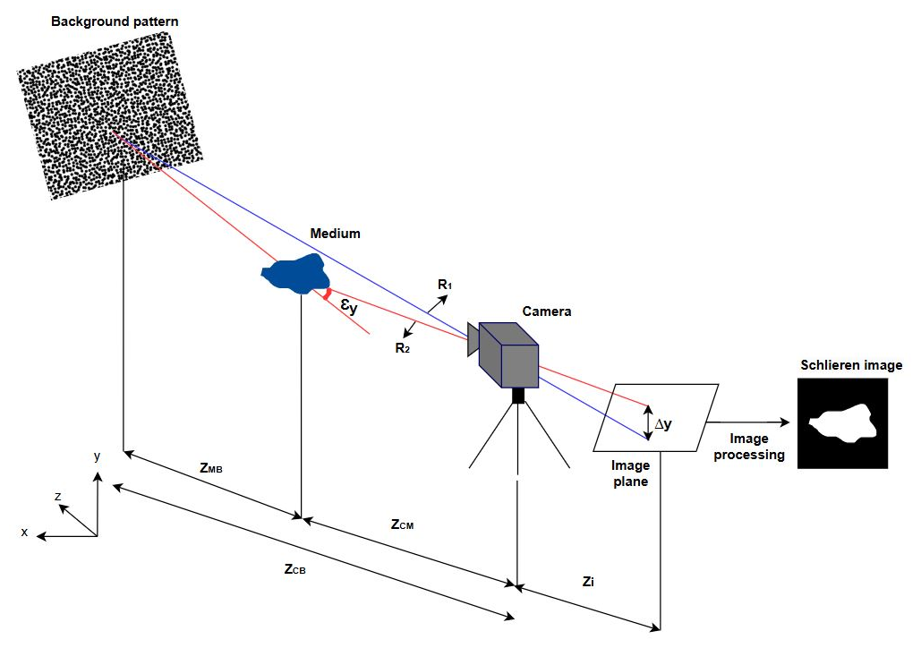
Figure 1 The schematic of the basic GSIS system setup – the basic GSIS setup uses a digital camera and high-contrast pattern board. Without obstructions, light travels straight (R1), but a gas causes ray deflection (R2), shifting pixels in the image and producing schlieren images that reveal gas density variations.

The relationship between light-ray deflection, refractive-index gradient, and the resulting image–plane displacement follows standard BOS theory based on geometric optics and the Gladstone–Dale relation (Settles, 2001; Raffel et al., 2007; Raffel et al., 2018) and is summarized in Eq. (3). The complete derivation is provided in Appendix A.

$$\begin{array}{}\text{(1)}& \mathbf{\Delta }\mathit{d}=f\left({\displaystyle \frac{Z_{\mathrm{MB}}}{Z_{\mathrm{CM}}+Z_{\mathrm{MB}}-f}}\right)\mathit{\epsilon }\end{array}$$

In the above, (f) is the focal length, (Z_CM) is the distance between the camera and medium, and (Z_MB) is the distance between medium and background (Z_MB).

2.2 3D-GSIS system road and lab setups

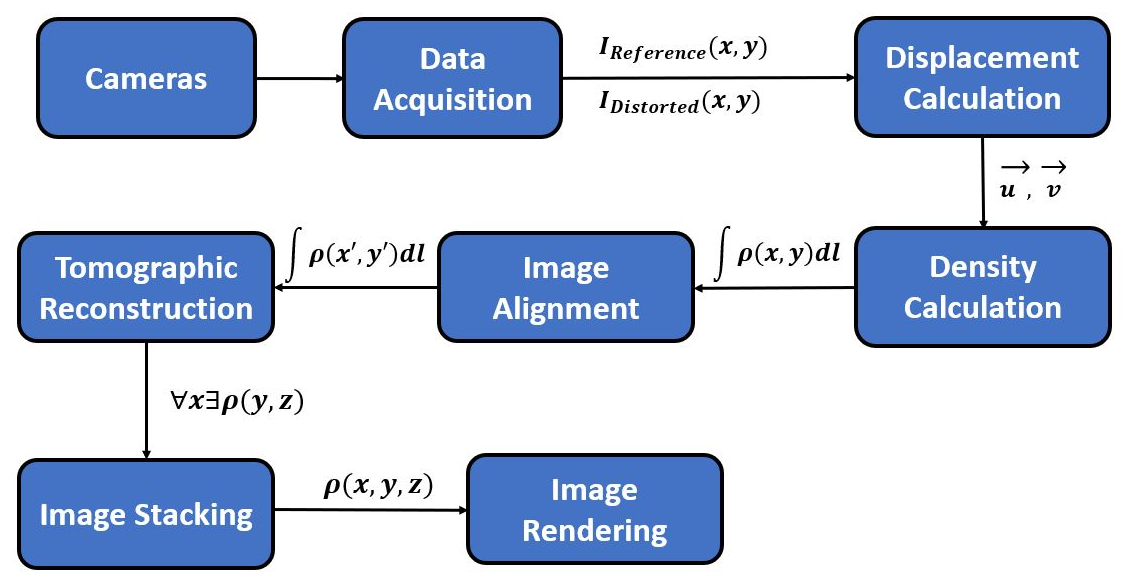
The 3D-GSIS system uses a truss-mounted array of six Raspberry Pi high-quality cameras, distributed evenly over a 100° viewing angle (40 to 140°) and focused on a random-dot background as shown in Fig. 2. For vehicles with low tailpipes, a 4 mm nozzle is attached to the exhaust, as shown in Fig. 3, while green-marked pipes help adjust for minor camera misalignment (see Sect. 2.5). The aluminum frame is 202 cm high and 154.4 cm wide, with cameras positioned at regular angular intervals ($\mathit{\theta }=[\mathrm{40},\mathrm{60},\mathrm{\dots },\mathrm{140}\mathit{°}]$), as illustrated in Fig. 3a. Each camera module features a 12.3-MP Sony IMX477R sensor and a 16 mm lens, all controlled by Raspberry Pi 4B units. Figure 4 shows the schematic of the work flow of 3D-GSIS system.

The system connects wirelessly through a local Wi-Fi hotspot, which allows for remote control and secure file transfers. Images from all cameras can be captured at the same time using an external trigger. Each camera is focused on a background pattern placed on the ground. The system is built to reconstruct the density of exhaust plumes in cylindrical spaces up to 31 cm wide and 41 cm high. Accurate results depend on careful camera placement. To reduce errors, the rotation axis is lined up with each camera's nodal point using custom 3D-printed mounts and nodal slide tests. Any small misalignments can be fixed in software.

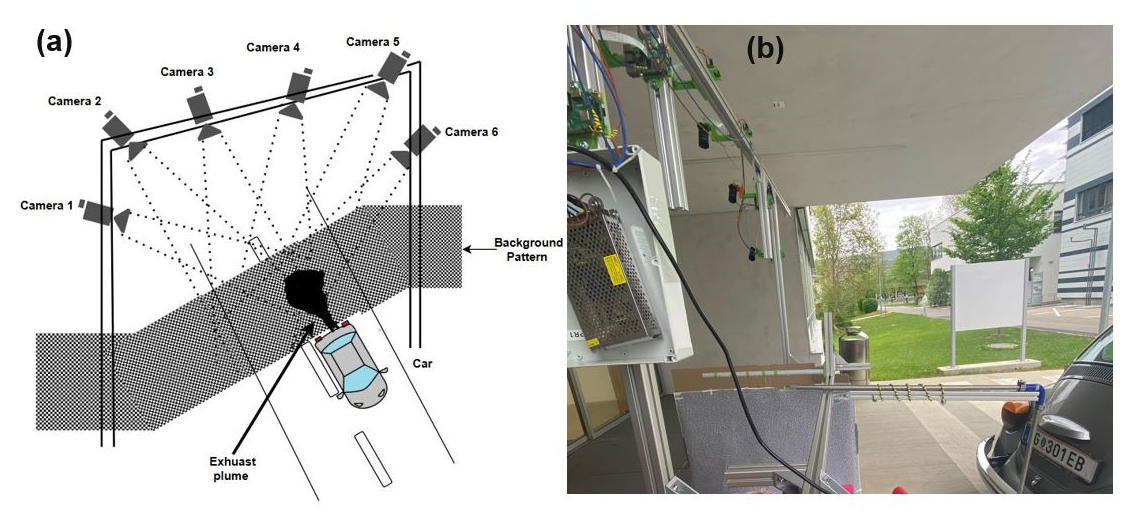
Figure 2 The 3D-GSIS system road setup – it consists of an equally distributed array of cameras mounted on a truss and covers a viewing angle of 100° (40 to 140°) and a random-dot pattern as the background. (a) Schematic representation and (b) original setup.

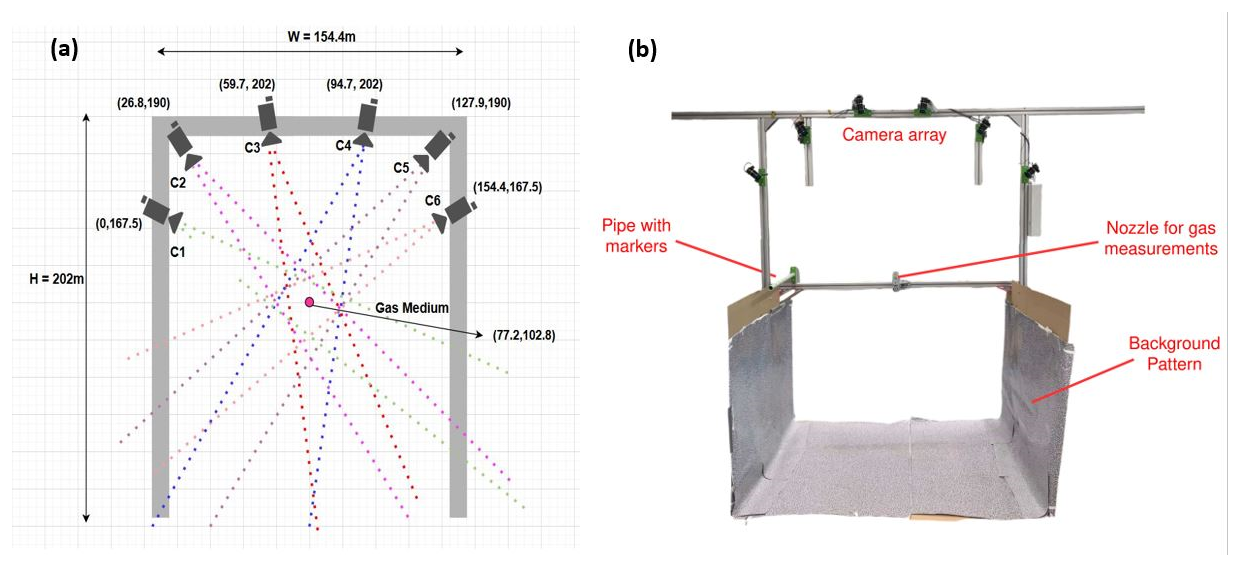
Figure 3 The 3D-GSIS system lab setup – it consists of an equally distributed array of cameras mounted on a truss and covers a viewing angle of 100° (40 to 140°), a random-dot pattern as the background, and a 4 mm nozzle designed for gas measurements, along with a pipe marked with green indicators to adjust for any remaining camera misalignment. (a) Schematic representation and (b) original setup.

Figure 4 The schematic of the workflow of the 3D-GSIS system.

2.3 Construction of displacement fields and calculation of displacements

BOS imaging quantifies exhaust plume dimensions by measuring image–plane displacements induced by refractive-index gradients between the exhaust gas and ambient air. The displacement magnitude and direction are determined using image-processing techniques applied to a reference image and a disturbed image containing the plume.

Two methods were implemented for displacement estimation. The first is digital image correlation (DIC) (Sutton et al., 2009), in which both images are divided into interrogation windows and cross-correlated using a random-dot background as a unique pattern. The displacement field is obtained from the peak correlation shifts between corresponding windows.

The second method is the Gunnar Farnebäck optical-flow algorithm (Farnebäck, 2003), which estimates dense motion fields using a polynomial expansion over an image pyramid of images at different resolutions. Displacements are iteratively refined across pyramid levels to obtain the final motion field.

2.4 Displacement to density fields/density calculation

The displacement gradients obtained from the BOS evaluation are related to the line-of-sight-integrated density field through a Poisson equation derived from geometric optics and the Gladstone–Dale relation. The detailed derivation is provided in Appendix B.

The governing equation for the two-dimensional line-integrated density field ${\mathit{\rho }}^{\ast }\left(x,y\right)$ is expressed as follows:

$$\begin{array}{}\text{(2)}& {\displaystyle \frac{{\partial }^{\mathrm{2}}}{\partial x^{\mathrm{2}}}}{\mathit{\rho }}^{\ast }\left(x,y\right)+{\displaystyle \frac{{\partial }^{\mathrm{2}}}{\partial y^{\mathrm{2}}}}{\mathit{\rho }}^{\ast }\left(x,y\right)=D\left(x,y\right),\text{(3)}& {\displaystyle }D(x,y)={\displaystyle \frac{(Z_{\mathrm{CM}}+Z_{\mathrm{MB}}-f)n_{\mathrm{0}}}{Z_{\mathrm{MB}}fG\left(\mathit{\lambda }\right)}}\left({\displaystyle \frac{\partial \mathrm{\Delta }x}{\partial x}}+{\displaystyle \frac{\partial \mathrm{\Delta }y}{\partial y}}\right).\end{array}$$

Here, ${\mathit{\rho }}^{\ast }\left(x,y\right)$ represents the line-of-sight-integrated density, while D(x,y) is the source term obtained from the spatial derivatives of the displacement components (Δx,Δy) together with the geometric parameters of the BOS setup. After computing the source term, the Poisson equation is solved numerically to recover ${\mathit{\rho }}^{\ast }\left(x,y\right)$.

To correctly evaluate the source term, the camera-to-background and camera-to-medium distances (Z_CM and Z_MB) are determined for each pixel based on the viewing geometry. Minor residual misalignments are reduced by spatially averaging these distance estimates. The ambient density is calculated from measured temperature, pressure, and relative humidity.

For computational efficiency, the images are downsampled by a factor of 4 (2560 × 1920 to 640 × 480). The Poisson equation is then solved using a parallel finite-difference scheme, following standard numerical approaches (Settles, 2001; Hargather and Settles, 2012). Dirichlet boundary conditions are applied at the upper and lower boundaries, while Neumann conditions are used along the lateral boundaries, consistently with the assumed density behavior at the domain edges.

2.5 Image alignment

For accurate tomographic reconstruction, BOS images from all cameras must be aligned in the same coordinate system. In this setup, alignment is made easier by mounting the cameras on a rigid truss, which keeps lens distortion and paraxial error very low. Any small misalignments that remain are corrected using geometric transformations such as rotation, translation, and scaling.

A calibration pipe with five visible markers is placed along the center of the measurement area, lined up with the gas nozzle axis (Fig. 3b). The positions of these markers are used to set a common reconstruction axis for all camera views. Unlike full camera calibration methods such as the Perspective-n-Point (PnP) approach for estimating camera pose in 3D space (Hartley and Zisserman, 2004), this method uses 2D geometric alignment of the image planes since the camera positions are fixed by the mounting setup.

To find the transformation parameters, the background pattern is removed first to make it easier to detect the markers. The markers are separated using a binary mask, and their contours are used to find the centroids. These centroids are then used to calculate the rotation, translation, and scaling needed to align each image to the shared reconstruction axis. Because the camera positions and angles are fixed by the mounting structure, the alignment only needs to correct small misalignments in the image plane. This marker-based alignment does not need to solve for the full 3D camera pose; it just makes sure the reconstruction axis is lined up the same way in all camera views. The alignment process is shown in Figs. 5 and 6.

Figure 5 Illustration of aligning camera data to a common reference axis.

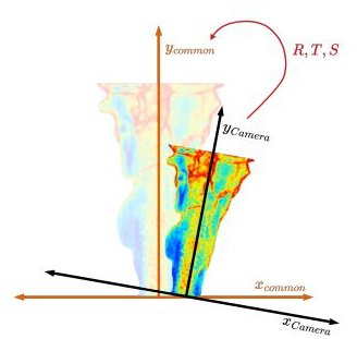
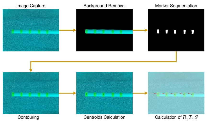
Figure 6 Procedure for estimating rotation (R), translation (T), and scale (S) to compensate for misalignments.

2.6 Tomographic density reconstruction

The line integral calculated for a camera indicates the cumulative density along the medium in the direction of the camera's line of sight. The density can be reconstructed by combining line integrals obtained from multiple viewing angles, following the fundamental principles of tomography (Andersen and Kak, 1984; Kak and Slaney, 1988; Zaman, 2022). These tomographic approaches have been widely applied in BOS-based three-dimensional density reconstruction, as demonstrated in previous studies (Atcheson et al., 2008; Nicolas et al., 2016; Amjad et al., 2023). In this work, projections from the multi-camera GSIS setup are used to reconstruct the three-dimensional density field of the exhaust plume.

2.6.1 Forward projection

Forward projection is the process of forming projection data through integrating the density field along rays that pass through the measurement volume. This process is described mathematically by the Radon transform, which creates a projection Pθ(t) for a specific viewing angle θ. Each projection shows the line integral of the density along parallel rays that cross the object. In the Supplement (Fig. S2), shows how forward projection is used in this study.

2.6.2 Simultaneous algebraic reconstruction technique (SART)

The simultaneous algebraic reconstruction technique (SART) is used to reconstruct the density distribution from measured projections (Andersen and Kak, 1984; Kak and Slaney, 1988). SART works by repeatedly updating the density field to reduce the difference between the measured projections and those calculated from the current estimate.

Unlike analytical methods like filtered back projection, iterative techniques such as SART work better for limited-angle tomography and when there are only a few projection datasets. This is important for our system, which uses only a small number of cameras. In each iteration, projection errors are spread along the related rays, and the density estimate is updated until the results stop changing.

This iterative process makes the reconstruction more stable and helps reduce artifacts that come from limited angular sampling. A detailed explanation of the SART algorithm and a schematic of the reconstruction procedure are provided in the Supplement (Sect. S1 and Fig. S3).

2.6.3 Implementation of SART algorithm

Reconstructing density distribution with the SART algorithm requires creating sinograms for each cross-section. Each camera captures multiple cross-sections, and each pixel column corresponds to a different cross-section at a specific angle. Aligned data are merged to form sinograms. The detailed description is present in the Supplement (Sect. S2 and shown in Fig. S4).

The SART algorithm works on a 2D grid, measuring reconstruction volume in pixels rather than physical units. Line integrals are first normalized to the length of rays intersecting the volume and then are adjusted for the algorithm's discretized space. A key challenge is that these integrals often include areas outside the actual reconstruction volume (see Fig. 7, blue area), leading to potential errors if not corrected as the algorithm assumes a uniform circular reconstruction area for every angle.

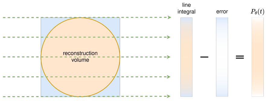
Figure 7 Illustration showing that computed line integrals (projections) may include contributions from regions outside the reconstruction volume, especially at oblique angles.

Sinogram correction relies on boundary conditions for the density outside the reconstruction area. The parallel-ray approximation, used in BOS and SART, simplifies this process. By projecting only the blue area (see Fig. 7), a corrective sinogram is created and subtracted to limit the integrals to the reconstruction volume.

To test the algorithm with limited-angle data, we used a simulated gas flow cross-section to generate sinograms in three ways: with 180 full-angle projections, with six limited angles, and with interpolated or extrapolated sinograms extended to 180 angles. Interpolation and extrapolation improved the reconstruction quality compared to using only six projections. For the final reconstruction, we applied one SART iteration to the extended sinograms and then used Gaussian filtering with scikit-image.

The current implementation requires approximately 10–20 s per reconstruction and about 1–2 min per dataset on a standard workstation and is therefore not optimized for real-time operation. However, the computational steps are suitable for parallelization and could be accelerated using GPU in future implementations.

2.7 Image stacking and rendering

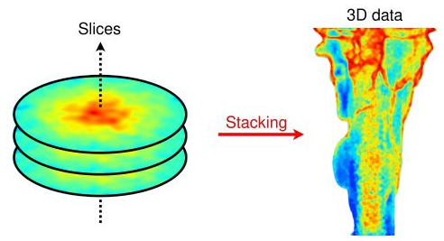
To obtain the three-dimensional density distribution, the reconstructed two-dimensional slices are stacked along the measurement axis, forming a volumetric dataset as shown in Fig. 8. In tomographic BOS with only a few projections, it is important to limit the reconstruction area to the actual region of interest to reduce streak artifacts. A spatial mask is used to focus the reconstruction on the measurement volume that contains the exhaust plume. This mask is generated by applying a threshold to the reconstructed density field and then refining it with a hole-filling step to keep the masked region continuous.

For visualization, the processed volume is displayed using PyVista, a Python interface to the Visualization Toolkit (VTK). The density field can be displayed with either volume rendering or by extracting surfaces. When extracting surfaces, iso-surfaces for different density levels are created using the marching cubes algorithm.

Figure 8 The 3D volume reconstruction by stacking sequential 2D image slices.

2.8 Modeling the gas schlieren imaging technique

A simulation model for the gas Schlieren imaging technique was developed using mixtures of different concentrations of air and CO₂. Displacements in the image plane were calculated to verify the results obtained from image-processing techniques. The overall model consists of two COMSOL models that are processed sequentially in Python. The first model conducts flow simulations of various concentrations of CO₂ injected into the air. The second model functions as a reverse pinhole camera for light propagation and ray tracing. In this model, rays emanating from the camera are traced as they pass through the gas flows. The light rays deflect based on the refractive-index gradient present along their path. The starting and ending points of the rays are recorded in two scenarios: when there is no gas flow and when gas flows are present. The displacements for each ray are then estimated.

The presented workflow combines multi-view BOS measurements with tomographic reconstruction to obtain the spatial density distribution of exhaust plumes. The reconstructed density field enables estimation of the effective absorption path length, which is required for quantitative remote emission sensing.

2.9 Ground truth data

We tested the DIC and OF algorithms for BOS imaging by making synthetic images with random-dot patterns. Using GIMP (GNU Image Manipulation Program), we introduced known rotational and translational movements into the patterns. Each algorithm processed these same images, and we checked how closely their results matched the expected displacement values.

3 Results and discussion

3.1 Displacement calculation and displacement field reconstruction

The DIC and OF algorithms for BOS imaging were evaluated using synthetic images containing random-dot patterns. Known rotational and translational movements were introduced into these patterns using GIMP (GNU Image Manipulation Program). Each algorithm processed the same set of images, and the accuracy of their results was assessed by comparing the measured displacements to the expected values. Pixel displacements ranging from 0.5 to 5 pixels were introduced and tested with both algorithms. The results are presented in Fig. 9. The x axis represents the ground truth pixel displacement, while the y axis indicates the relative error in percentage. Blue dots correspond to the measured displacement relative error using OF, and orange dots represent the error using DIC. The OF algorithm demonstrates a mean relative error of 0.04 % across all distances, whereas DIC exhibits a mean relative error of 1.9 %. Similar evaluations were conducted for rotational displacements, where OF again outperforms DIC, showing a relative error of 6.49 % compared to DIC's 17.62 %. These results are provided in the Supplement (Fig. S5). Based on these findings, the OF algorithm is used in subsequent measurements.

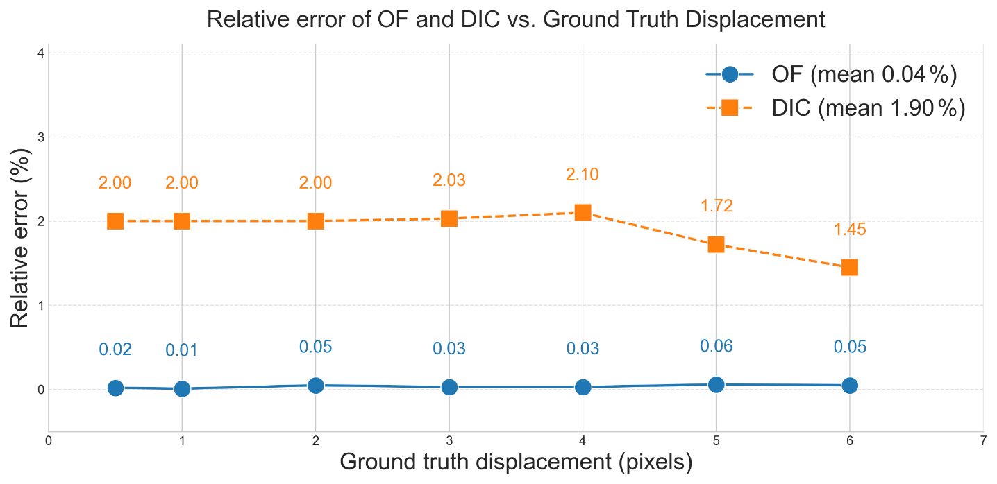
Figure 9 Relative error of displacement estimated using optical flow (OF) and digital image correlation (DIC) with respect to the ground truth

To test the 3D-GSIS system in the lab, a mixture of air and CO₂ at different concentrations was used. The accuracy of the density field reconstruction relies on how precisely we calculate the displacements in the camera images. The setup included a transparent acrylic gas container measuring 100 cm × 60 cm × 60 cm. Gas was supplied from pressurized bottles at a rate of 6 L min⁻¹. We used a tube furnace from Carbolite Gero GmbH & Co. KG to heat the gases and a gas diluter to control the concentration. Inside the container, we monitored temperature, pressure, and humidity. A camera was aimed at a pattern board placed on the opposite side of the container. We took a reference image without gas flow and then captured images during gas flow at 90 frames per second (640 × 480 pixels). We analyzed the reference and flow images using the OF algorithm to determine the gas flow displacement fields. Pixel displacement was calculated directly from the images using the gas schlieren imaging technique described in Sect. 2.3. The pixel displacement values from the simulation model, described in Sect. 2.8, were used as reference data. Figure 10 shows the reconstructed displacement field for gas flow with 70 % CO₂, where (a) represents the closer view of the displacement field of the background, and (b) represents the closer view of the displacement field of the region where gas flow has maximum density. Figure 11 presents the histogram of pixel displacement magnitudes. Most pixels exhibit very small displacements, representing the background, while a smaller number show much larger displacements caused by the gas plume. These larger values are due to refractive-index gradients in the plume. We compared the BOS-measured displacements with values predicted by the COMSOL simulation model. For comparison, we selected an area of pixels in the flow region where the density is maximum and calculated the average displacement of the pixels in this region. Linear regression analysis produced $y=\mathrm{0.951}x+\mathrm{0.012}$, signifying a strong correlation between simulation and measurement with only a small systematic difference, as shown in Fig. 12. The RMSE was 0.013 pixels, indicating a low overall error relative to the measured displacement range. This result shows that the BOS method provides reliable and accurate displacement measurements for the tested CO₂ concentrations.

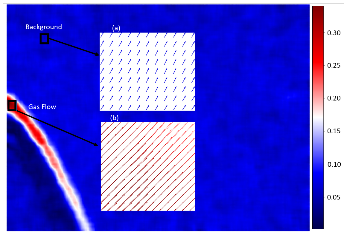
Figure 10 Reconstructed displacement field of a gas flow containing 70 % CO₂ – (a) closer view of the background and (b) closer view of the gas flow.

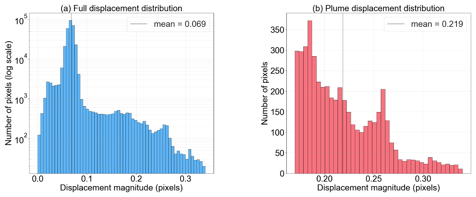
Figure 11 Histogram of displacement values: (a) full displacement distribution and (b) plume-only displacement distribution.

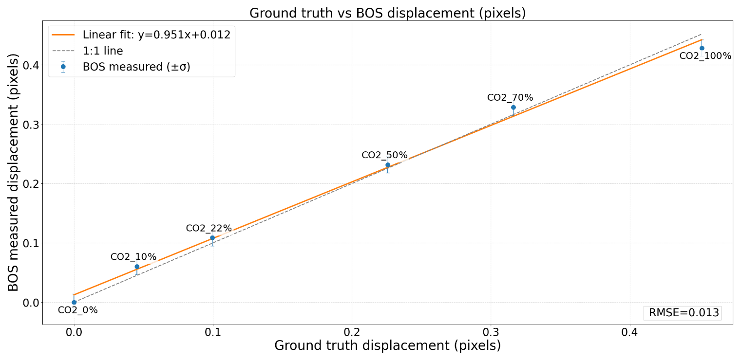
Figure 12 Ground truth vs. BOS-measured displacement for different concentrations of CO₂. A linear fit ($y=\mathrm{0.951}x+\mathrm{0.012}$) shows good agreement, with an RMSE of 0.013.

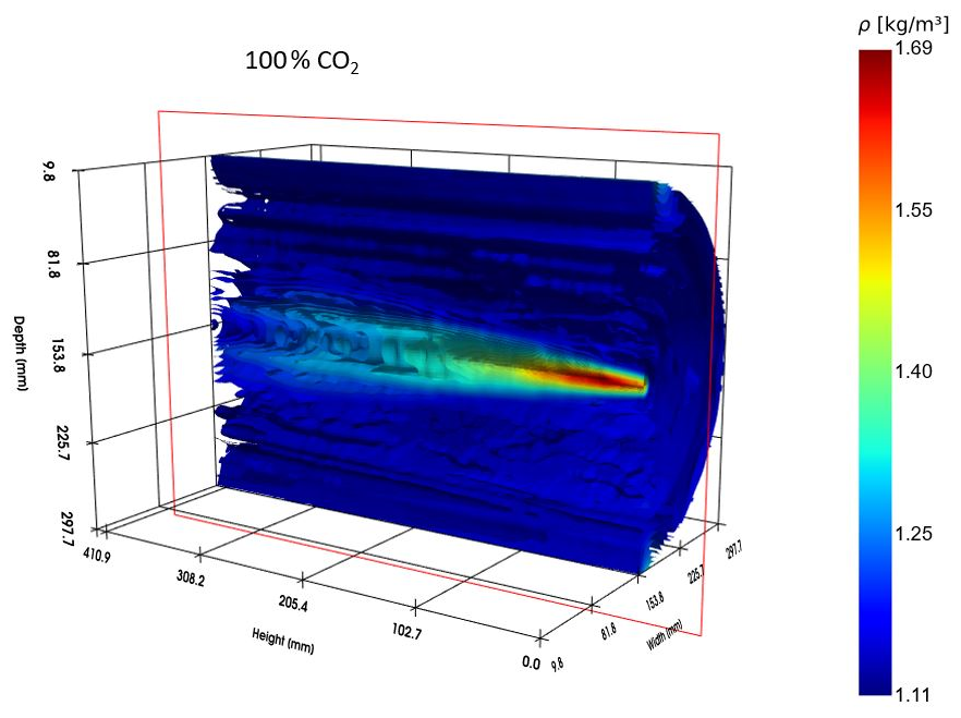
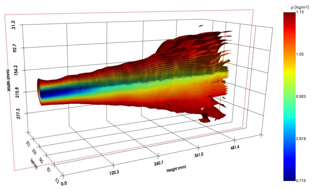
3.2 The 3D density field reconstruction of gas flows and hot air

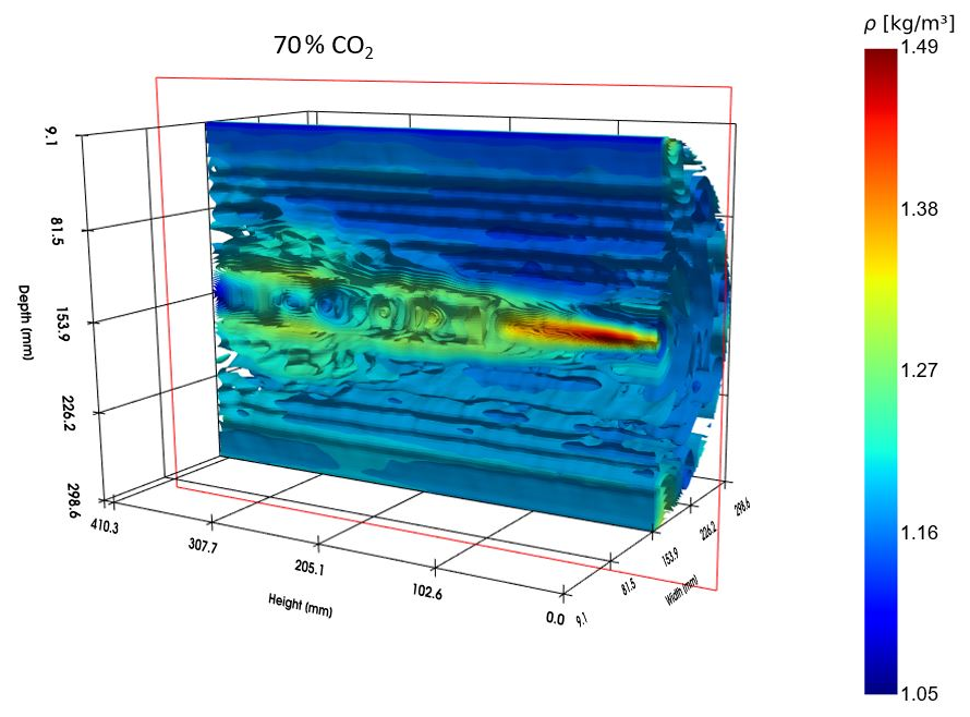
For different concentrations of CO₂ – 50 %, 70 %, and 100 % – the 3D density fields of gas flows can be reconstructed; also, the density of the gas flow was obtained in kg m⁻³. The 3D density fields of gas flows with a 70 % and 100 % concentration of CO₂ are shown in Figs. 14 and 15. The density fields of gas flows with other concentrations are shown in the Supplement (Fig. S1). The calculated theoretical values and experimental values of the density of gas flows are shown in Table 2. The results show that the calculated density values of gas flows using the 3D-GSIS system show a relative error concerning ground truth displacement values in the 2 % to 3 % range. The linear fit, $y=\mathrm{0.947}x+\mathrm{0.037}$, shown in Fig. 13, indicates that the measurements closely follow the expected values, with only a small difference. The RMSE is 0.049, which means the overall error across the tested range is low. These results suggest that the reconstructed density field can be used reliably for path length estimation.

It can be seen from the reconstructed density fields of the gas flows that high-density gradients are most prominent at the nozzle exit, gradually decreasing as the gas disperses into the surrounding atmosphere. This behavior results in an expanding plume diameter, consistently with fluid dynamic expectations. Within the core region of the jet, the density gradients remain relatively strong due to limited mixing and entrainment. At lower gas concentrations, the plume becomes increasingly diffuse, making it more difficult to distinguish from the background. This reduction in contrast adversely affects reconstruction accuracy as weaker density gradients are more susceptible to image noise. Furthermore, as the ambient and gas densities converge, the resulting decline in image gradient strength reduces the effectiveness of optical-flow algorithms and increases the influence of noise on the measured flow field.

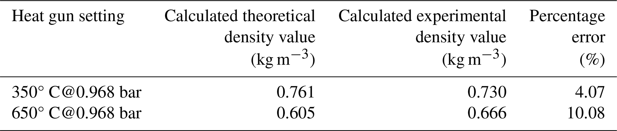
Experiments using hot air at different temperatures have also been conducted. A heat gun was utilized to generate hot air jets at temperatures of 350 and 650 °C. To calculate the density of the hot air, measurements were taken under ambient conditions of temperature, humidity, and pressure. The reconstructed density field of the hot-air plume at 350 °C is shown in Fig. 16. The calculated density values are shown in Table 3. The results indicate that the calculated density values have a relative error of 4 % to 10 % compared to the theoretical values. These values are determined very close to the nozzle.

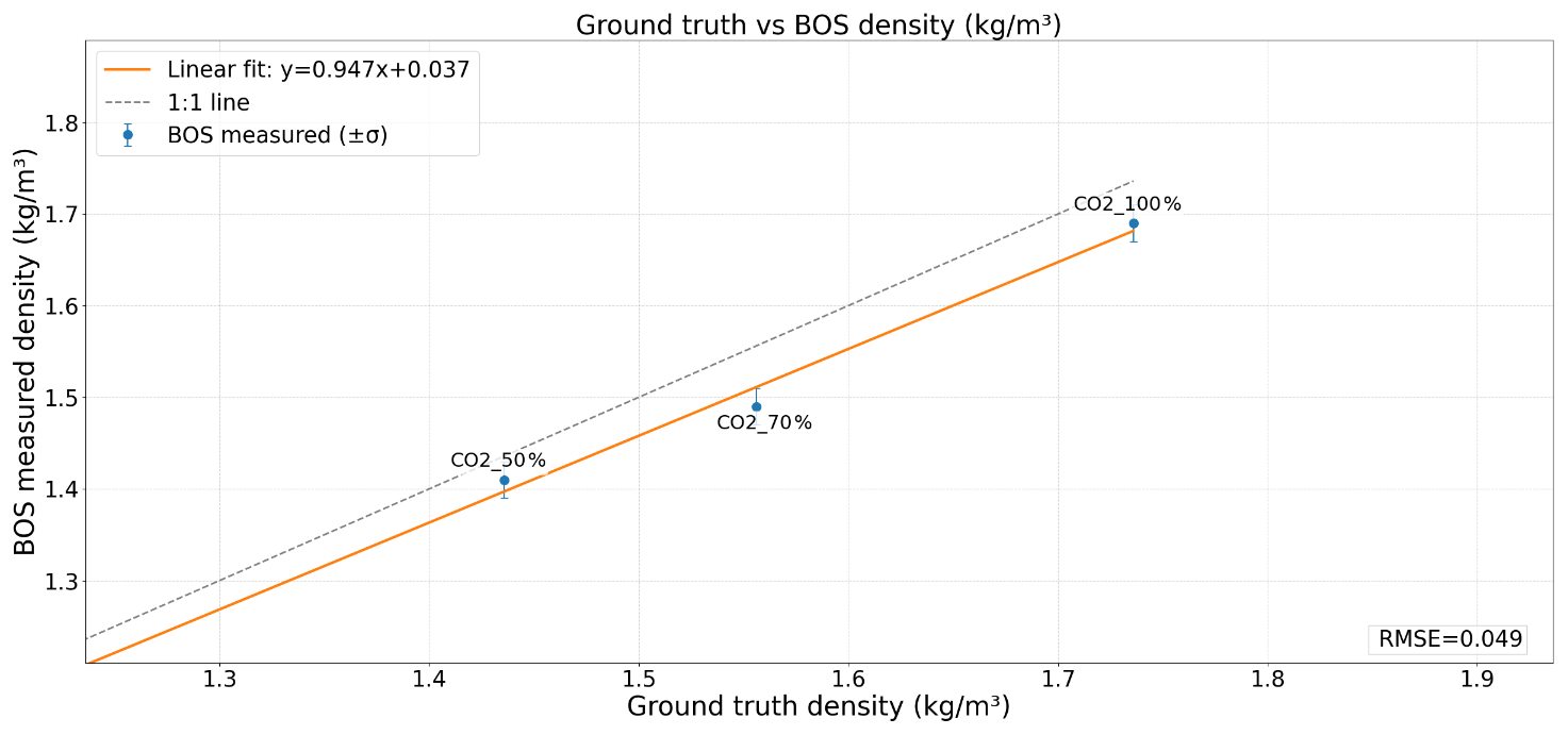
Figure 13 Ground truth vs. BOS-measured density for different concentrations of CO₂. A linear fit ($y=\mathrm{0.947}x+\mathrm{0.037}$) shows good agreement, with an RMSE of 0.049.

Table 1 Comparison of calculated and actual density values for different CO₂ concentrations.

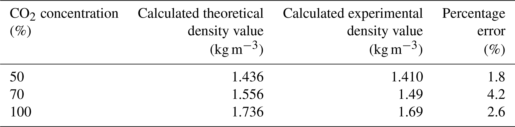
Table 2 Comparison of calculated and actual density values for different temperatures.

Figure 14 Cross-sectional density distribution resulting from a 70 % carbon dioxide flow.

Figure 15 Cross-sectional density distribution resulting from a 100 % carbon dioxide flow.

Figure 16 Cross-section of the reconstructed density distribution at 350 °C.

3.3 The 3D density field reconstruction and path length estimation of exhaust plumes

3.3.1 Validation of plume size and absorption path length estimation

To evaluate how well the system can estimate plume dimensions and absorption path length, a simple and controlled validation experiment was performed using a pipe with an outer diameter of 25 mm. Due to the wall thickness, the internal diameter is approximately 22 mm, which represents the expected diameter of the gas flow at the outlet. The reconstructed 3D density field was then used to estimate the plume diameter close to the pipe exit, where the flow is still well-defined. From the reconstruction, a diameter of about 21.25 mm was obtained. This is reasonably close to the expected internal diameter. The deviation is relatively small and is summarized in Table 3. In addition, Fig. 17 shows the reconstructed plume, which visually supports the diameter and absorption path length estimation. Overall, the results suggest that the 3D-GSIS system is able to capture the plume size with acceptable accuracy and can be used for path length estimation.

Table 3 Validation of absorption path length estimation.

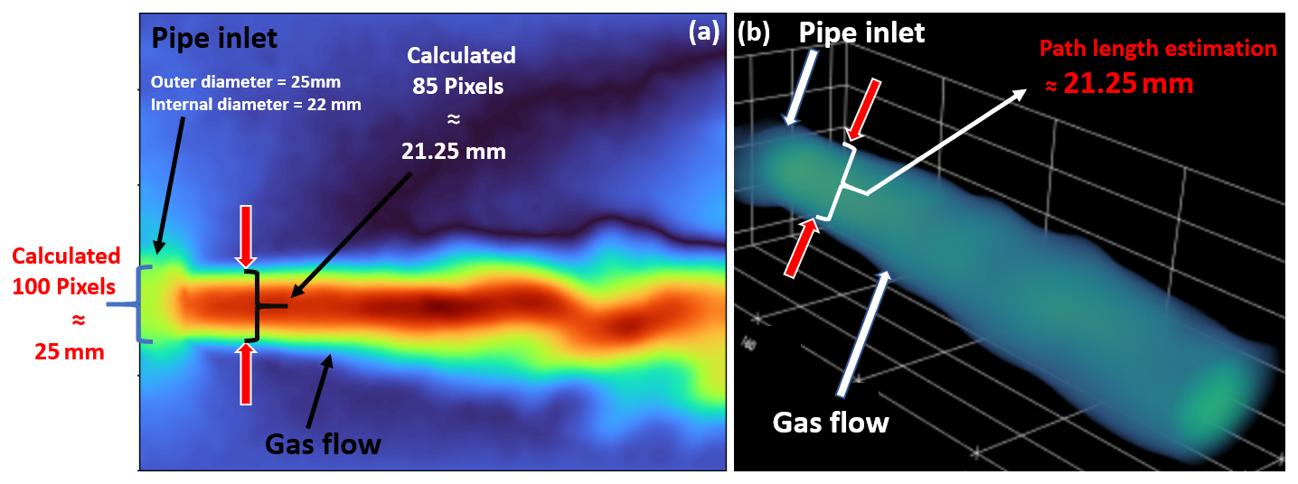
Figure 17 Validation of absorption path length estimation: (a) reconstructed 2D line-of-sight-integrated density field and calculated plume size and (b) reconstructed 3D density field and calculated absorption path length.

3.3.2 Application to vehicle exhaust plumes

The two-camera-based 3D gas schlieren imaging sensor (3D-GSIS) system was implemented at the AVL List GmbH test track in Graz, Austria, and at Donkerstraat in Leuven, Belgium, as part of the emission measurement campaign under the LENS project (LENS Project Consortium, 2025). It was not feasible to transport and set up a six-camera-based 3D-GSIS system at these testing sites due to spatial constraints related to the width of the test track and measurement area. In both cases, the GSIS system with two cameras was installed horizontally along the roadside, capturing the exhaust plume. The density fields are reconstructed using the line of sight, assuming uniform density fields across all angles – this is feasible as the tailpipes are cylindrical. The 3D density field is then estimated through interpolation. While incorporating more cameras improves the accuracy of the estimation, it is important to note that the estimation of the 3D density field does not yield exact density values. Rather, it provides insight into how the exhaust plume is dispersed, allowing for calculations of the exhaust plume size in relation to the absorption path length from a single direction.

Various vehicles were examined by the 3D-GSIS system, and, in all cases, the 3D density fields have been successfully estimated. The original frames illustrating the vehicles passing in front of the pattern board and the positions of the tailpipes are presented in Fig. 18. In Fig. 18a, the passing vehicle is a car. In contrast, Fig. 18b and c show two motorcycles as the passing vehicles. The estimated reconstructed 3D density fields of the exhaust plumes of the three vehicles are displayed in Figs. 19, 20, and 21, respectively. The 3D density fields of exhaust plumes are rotated and displayed in the same direction for all vehicles. The estimated diameters in the middle of exhaust plumes are shown in Table 4.

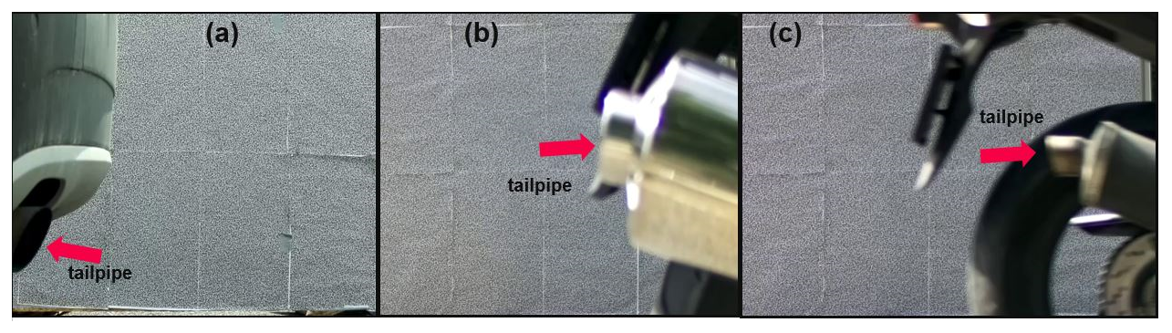
Figure 18 Original frames showing vehicles passing in front of the pattern board. (a) A car passing by. (b, c) Two motorcycles passing by with visible tailpipe positions.

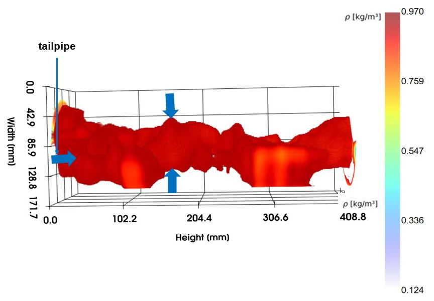
Figure 19 Estimated reconstructed density field of the exhaust plume from the passing car. The two opposite arrows indicate the center of the plume.

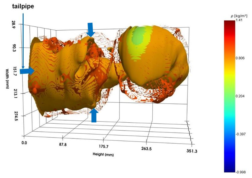
Figure 20 Estimated reconstructed density field of the exhaust plume from the passing motorcycle 1. The two opposite arrows indicate the center of the plume.

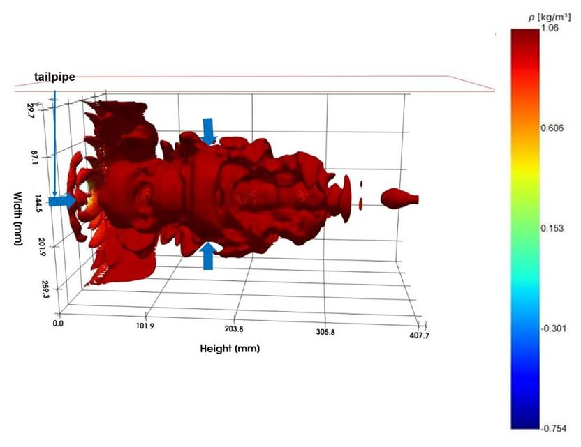
Figure 21 Estimated reconstructed density field of the exhaust plume from the passing motorcycle 2. The two opposite arrows indicate the center of the plume.

Table 4 Estimated size and absorption path lengths of the vehicle exhaust plumes.

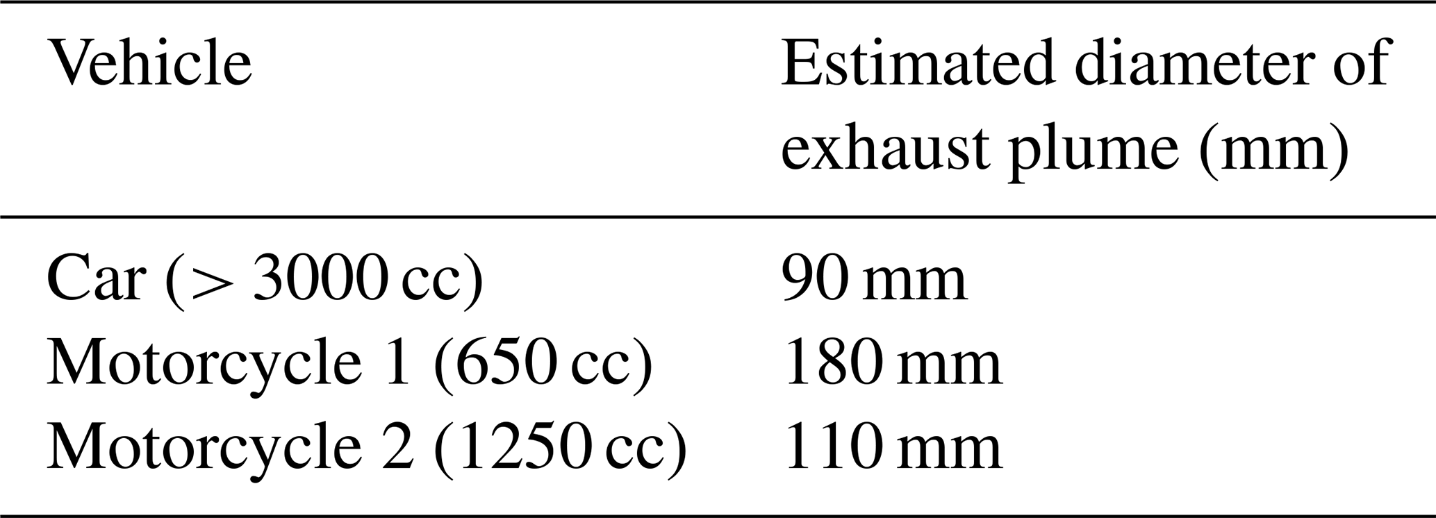
The size of exhaust plumes is not related to the concentration of pollutants in exhaust plumes. These plumes were captured from randomly passing vehicles operating under varying speeds, loads, and thrust conditions during the measurement. However, the estimated plume size provides important information about the absorption path length for the lasers used in advanced remote emission sensing (RES) devices.

4 Conclusions

In this work, we present a 3D gas schlieren imaging sensor (3D-GSIS) system that allows the reconstruction of 3D density fields of vehicle exhaust plumes for remote emission sensing applications. The system enables the calculation of the size of the vehicle exhaust plumes and the estimation of absorption path lengths of the lasers from both horizontal and vertical RES systems, which are typically unknown in conventional RES measurements. The combination of multi-view BOS and tomographic reconstruction, therefore, offers a practical way to link optical measurements with physically meaningful quantities required to determine direct pollutant concentrations from vehicle exhaust plumes rather than pollutant-to-CO₂ ratios. Moreover, it also provides information about the point where the laser intersects with the exhaust plume and the density of the exhaust plume at that point.

Results are presented from laboratory experiments at three different concentrations of CO₂ and from experiments with vehicle exhaust plumes at a test track and in traffic.

For the laboratory characterization of the 3D-GSIS system, a mixture of air and three different concentrations of CO₂ – 50 %, 70 %, and 100 % – was used, and the displacement and density fields have been successfully reconstructed. Displacement calculations from BOS images were performed using optical flow (OF) and digital image correlation (DIC) algorithms. The performance of these algorithms was evaluated based on synthetic images with predefined translational and rotational displacements. Results indicate that, for translational displacements, the OF algorithm achieves a mean relative error of 0.04 % across all distances, while DIC yields a mean relative error of 1.9 %. For rotational displacements, OF again outperforms DIC, with a relative error of 6.49 % compared to DIC's 17.62 %. Consequently, the OF algorithm was selected to reconstruct displacement fields of exhaust plumes.

A simulation model of the 2D gas schlieren imaging sensor system is developed, and displacements are calculated for different concentrations of CO₂ and have been compared with the displacement from the experimental evaluation. At 50 % CO₂, the calculated and ground truth displacement values show a relative error of 4.1 %, while, at 70 % and 100 %, the calculated and ground truth displacement values show a relative error of 4.0 % and 5.3 %, respectively. Linear regression analysis yielded the equation $y=\mathrm{0.951}x+\mathrm{0.012}$, indicating a strong link between simulation and measurement, with only a small systematic difference. The RMSE was 0.013 pixels, indicating a low overall error relative to the measured displacement range. These results show that the BOS method provides reliable, accurate displacement measurements across the tested CO₂ concentrations. Displacement histograms of the gas flow fields are shown, providing a clearer analysis of the distribution of pixel values within the measurement domain. While the histogram of the full field is dominated by background noise, the plume-specific distribution highlights higher displacement values associated with the gas flow. This supports the reliability of the displacement extraction and helps distinguish plume-induced signals from the background.

The 3D density fields of gas flows are reconstructed, and the density values of gas flow (in kg m⁻³) are also calculated with a 3D-GSIS system. The calculated theoretical and experimental values of the density of gas flows show relative errors of 1.8 %, 4.2 %, and 2.6 % at 50 %, 70 %, and 100 % concentrations of CO₂. The density fields of the hot-air jets at 350 and 650 °C have also been captured and reconstructed. The results indicate that the calculated density values have a relative error of 4 % to 10 % compared to the theoretical values. Linear regression analysis produced the equation $y=\mathrm{0.947}x+\mathrm{0.037}$, demonstrating a strong correlation between simulation and measurement, with minimal systematic deviation. The RMSE was 0.049 pixels, indicating a low overall discrepancy between the calculated and measured densities. The results indicate that the reconstructed density field provides a reliable basis for path length estimation.

To test the 3D-GSIS system's accuracy in estimating plume size and absorption path length, a validation experiment was conducted using a 25 mm diameter pipe. The internal diameter, accounting for wall thickness, is about 22 mm. The plume size calculated from the reconstructed density field closely matched the pipe's internal diameter. The measured value was 21.25 mm, close to the nominal 22 mm, yielding an error of about 3.4 %. The results show that the method can reliably measure the plume's physical size and provides a strong basis for estimating the effective absorption path length.

The two-camera 3D-GSIS system was used at roadside test sites in Austria and Belgium, where space constraints made a six-camera setup impractical. Despite this limitation, the system captured exhaust plumes from passing vehicles, which include cars and bikes, and reconstructed their 3D density fields from line-of-sight measurements. Although absolute density values could not be obtained, the results still provided useful information about plume shape, dispersion, and its relation to the absorption path. Overall, the measurements show that the 3D-GSIS approach can be applied under real conditions and can support the estimation of absorption path length in remote emission sensing.

Our research suggests that the 3D-GSIS system is capable of accurate reconstruction of the density distribution of tailpipe emissions. This is supported by laboratory measurements involving carbon dioxide and heat, which showed sufficient precision in density assessment and accurate absorption path length estimation of gas plume.

It must be noted that tailpipe emissions may primarily be detectable due to their elevated temperatures. Challenges arise when attempting to measure emissions from exhaust gases that have cooled significantly; the current lab setup struggled to identify lower concentrations of carbon dioxide.

The inaccuracies and low sensitivity of the current setup can be linked to the budget-friendly components used, including the cameras, lenses, and background patterns. For future studies, upgrading these components is essential. Moreover, the present configuration allows only for long exposure times, which leads to synchronization issues. Given that tailpipe emissions involve turbulent flows, exploring a new configuration for research may lead to more effective results and deeper insights. Investigating different background patterns could provide insights into their impact on measurement sensitivity and accuracy, especially given the current limitations in sensitivity. Additionally, modifying the setup's geometry according to the size of the road is necessary to enhance sensitivity and to improve the system's ability to capture tailpipe emissions. Finally, incorporating more cameras into the existing six-camera array could significantly boost measurement accuracy, given the current challenges with interpolation and extrapolation methods.

In the future, a 3D-GSIS system with more than six high-speed cameras and improved geometry will be developed to effectively cover the entire road from larger distances for passing vehicles. The 3D-GSIS system will be combined with the laser absorption spectroscopic-based RES system for the measurement of the direct concentration of pollutants in vehicle exhaust plumes.

Appendix A

The relation between the refractive index and density of the gaseous medium is given as

$$\begin{array}{}\text{(A1)}& n=\mathrm{1}+G\left(\mathit{\lambda }\right)\mathit{\rho },\end{array}$$

where n is the refractive index of the gaseous medium, G is the Gladstone–Dale constant, and ρ is the density of the medium. The value of the Gladstone–Dale constant depends on the wavelength (λ) of the light in use.

The deflection angle can be calculated by integrating the refractive-index gradients along the line of sight, as shown in Eq. (A2).

$$\begin{array}{}\text{(A2)}& \mathit{\epsilon }={\displaystyle \frac{\mathrm{1}}{n_{\mathrm{0}}}}\underset{z_{\mathrm{MB}}-\mathrm{\Delta }{z}_{\mathrm{MB}}}{\overset{z_{\mathrm{MB}}+\mathrm{\Delta }{z}_{\mathrm{MB}}}{\int }}\mathrm{\nabla }n\mathrm{d}z.\end{array}$$

Here, n₀ is the refractive index of the surrounding air, and ∇n is the refractive-index gradient of the gaseous medium with the refractive index (n), as shown in Eq. (A3).

$$\begin{array}{}\text{(A3)}& \mathrm{\nabla }n={\left[\begin{array}{cc}\frac{\partial n}{\partial x}& \frac{\partial n}{\partial y}\end{array}\right]}^T\end{array}$$

The background pattern usually covers a significantly larger area than the image plane. Assuming only small deflection angles (ε_y≈tan ε_y) and paraxial approximation leads to the relationship between the ray displacements and the pixel displacements, as shown in the Eq. (A4).

$$\begin{array}{}\text{(A4)}& \mathbf{\Delta }\mathit{d}=Z_{\mathrm{MB}}M\mathit{\epsilon }\end{array}$$

Here, M is the magnification factor of the ratio of focal length (f=Z_i) to the distance of the camera to the board Z_CB, as shown in Eq. (A5), and Z_MB is the distance between the medium and background pattern board.

$$\begin{array}{}\text{(A5)}& M={\displaystyle \frac{Z_i}{Z_{\mathrm{CB}}}}\end{array}$$

By applying the thin-lens equation, M can be rewritten as shown in Eq. (A6).

$$\begin{array}{}\text{(A6)}& M={\displaystyle \frac{f}{Z_{\mathrm{CB}}-f}}\end{array}$$

The distance between the camera and pattern board (Z_CB) is equal to the distance between the camera and medium (Z_CM) plus the distance between the medium and background (Z_MB).

$$\begin{array}{}\text{(A7)}& Z_{\mathrm{CB}}=Z_{\mathrm{CM}}+Z_{\mathrm{MB}}\end{array}$$

Using Eqs. (A4), (A6), and (A7), the relationship between the ray and pixel displacements can be determined with known parameters and depends solely on the measurement setup as shown in Eq. (A8).

$$\begin{array}{}\text{(A8)}& {\displaystyle }\mathbf{\Delta }\mathit{d}=f\left({\displaystyle \frac{Z_{\mathrm{MB}}}{Z_{\mathrm{CM}}+Z_{\mathrm{MB}}-f}}\right)\mathit{\epsilon }\end{array}$$

Appendix B

$$\begin{array}{}\text{(B1)}& {\displaystyle }\mathbf{\Delta }\mathit{d}=f\left({\displaystyle \frac{Z_{\mathrm{MB}}}{Z_{\mathrm{CM}}+Z_{\mathrm{MB}}-f}}\right)\mathit{\epsilon }\text{(B2)}& {\displaystyle }\mathrm{\nabla }n=\mathrm{\nabla }\left(\mathrm{1}+G\left(\mathit{\lambda }\right)\mathit{\rho }\right)=G\left(\mathit{\lambda }\right)\mathrm{\nabla }\mathit{\rho }\text{(B3)}& {\displaystyle }\mathit{\epsilon }={\displaystyle \frac{G\left(\mathit{\lambda }\right)}{n_{\mathrm{0}}}}\underset{z_{\mathrm{MB}}-\mathrm{\Delta }{z}_{\mathrm{MB}}}{\overset{z_{\mathrm{MB}}+\mathrm{\Delta }{z}_{\mathrm{MB}}}{\int }}\mathrm{\nabla }\mathit{\rho }\mathrm{d}z\end{array}$$

After substituting Eq. (B3) into Eq. (B1), the displacement of pixels in the image plane can be written in terms of density, as shown in Eq. (B4).

$$\begin{array}{}\text{(B4)}& \mathbf{\Delta }\mathit{d}=f\left({\displaystyle \frac{Z_{\mathrm{MB}}}{Z_{\mathrm{CM}}+Z_{\mathrm{MB}}-f}}\right){\displaystyle \frac{G\left(\mathit{\lambda }\right)}{n_{\mathrm{0}}}}\underset{z_{\mathrm{MB}}-\mathrm{\Delta }{z}_{\mathrm{MB}}}{\overset{z_{\mathrm{MB}}+\mathrm{\Delta }{z}_{\mathrm{MB}}}{\int }}\mathrm{\nabla }\mathit{\rho }\mathrm{d}z\end{array}$$

Δd can be divided into x and y components, as shown in Eq. (B5) and (B6).

$$\begin{array}{}\text{(B5)}& {\displaystyle }\mathrm{\Delta }x=f\left({\displaystyle \frac{Z_{\mathrm{MB}}}{Z_{\mathrm{CM}}+Z_{\mathrm{MB}}-f}}\right){\displaystyle \frac{G\left(\mathit{\lambda }\right)}{n_{\mathrm{0}}}}\underset{z_{\mathrm{MB}}-\mathrm{\Delta }{z}_{\mathrm{MB}}}{\overset{z_{\mathrm{MB}}+\mathrm{\Delta }{z}_{\mathrm{MB}}}{\int }}{\displaystyle \frac{\partial \mathit{\rho }}{\partial x}}\mathrm{d}z\text{(B6)}& {\displaystyle }\mathrm{\Delta }y=f\left({\displaystyle \frac{Z_{\mathrm{MB}}}{Z_{\mathrm{CM}}+Z_{\mathrm{MB}}-f}}\right){\displaystyle \frac{G\left(\mathit{\lambda }\right)}{n_{\mathrm{0}}}}\underset{z_{\mathrm{MB}}-\mathrm{\Delta }{z}_{\mathrm{MB}}}{\overset{z_{\mathrm{MB}}+\mathrm{\Delta }{z}_{\mathrm{MB}}}{\int }}{\displaystyle \frac{\partial \mathit{\rho }}{\partial y}}\mathrm{d}z\end{array}$$

After first partially differentiating the pixel displacements with respect to their corresponding directions, Eqs. (B5) and (B6) can be written as shown below.

$$\begin{array}{}\text{(B7)}& {\displaystyle }\begin{array}{rl}{\displaystyle \frac{\partial \mathrm{\Delta }x}{\partial x}}& =f\left({\displaystyle \frac{Z_{\mathrm{MB}}}{Z_{\mathrm{CM}}+Z_{\mathrm{MB}}-f}}\right){\displaystyle \frac{G\left(\mathit{\lambda }\right)}{n_{\mathrm{0}}}}\\ & {\displaystyle \frac{{\partial }^{\mathrm{2}}}{\partial x^{\mathrm{2}}}}\underset{z_{\mathrm{MB}}-\mathrm{\Delta }{z}_{\mathrm{MB}}}{\overset{z_{\mathrm{MB}}+\mathrm{\Delta }{z}_{\mathrm{MB}}}{\int }}\mathit{\rho }\mathrm{d}z\end{array}\text{(B8)}& {\displaystyle }\begin{array}{rl}{\displaystyle \frac{\partial \mathrm{\Delta }y}{\partial y}}& =f\left({\displaystyle \frac{Z_{\mathrm{MB}}}{Z_{\mathrm{CM}}+Z_{\mathrm{MB}}-f}}\right){\displaystyle \frac{G\left(\mathit{\lambda }\right)}{n_{\mathrm{0}}}}\\ & {\displaystyle \frac{{\partial }^{\mathrm{2}}}{\partial y^{\mathrm{2}}}}\underset{z_{\mathrm{MB}}-\mathrm{\Delta }{z}_{\mathrm{MB}}}{\overset{z_{\mathrm{MB}}+\mathrm{\Delta }{z}_{\mathrm{MB}}}{\int }}\mathit{\rho }\mathrm{d}z\end{array}\text{(B9)}& {\displaystyle }\begin{array}{rl}{\displaystyle \frac{\partial \mathrm{\Delta }x}{\partial x}}& +{\displaystyle \frac{\partial \mathrm{\Delta }y}{\partial y}}=f\left({\displaystyle \frac{Z_{\mathrm{MB}}}{Z_{\mathrm{CM}}+Z_{\mathrm{MB}}-f}}\right){\displaystyle \frac{G\left(\mathit{\lambda }\right)}{n_{\mathrm{0}}}}\\ & \left[{\displaystyle \frac{{\partial }^{\mathrm{2}}}{\partial x^{\mathrm{2}}}}\underset{z_{\mathrm{MB}}-\mathrm{\Delta }{z}_{\mathrm{MB}}}{\overset{z_{\mathrm{MB}}+\mathrm{\Delta }{z}_{\mathrm{MB}}}{\int }}\mathit{\rho }\mathrm{d}z+{\displaystyle \frac{{\partial }^{\mathrm{2}}}{\partial y^{\mathrm{2}}}}\underset{z_{\mathrm{MB}}-\mathrm{\Delta }{z}_{\mathrm{MB}}}{\overset{z_{\mathrm{MB}}+\mathrm{\Delta }{z}_{\mathrm{MB}}}{\int }}\mathit{\rho }\mathrm{d}z\right]\end{array}\end{array}$$

Assuming ${\int }_{z_{\mathrm{MB}}-\mathrm{\Delta }{z}_{\mathrm{MB}}}^{z_{\mathrm{MB}}+\mathrm{\Delta }{z}_{\mathrm{MB}}}\mathit{\rho }\mathrm{d}z={\mathit{\rho }}^{\ast }\left(x,y\right)$, Eq. (B9) can be written as a Poisson equation, which can subsequently be solved for the line integral of the medium's density, as shown below.

$$\begin{array}{}\text{(B10)}& {\displaystyle \frac{{\partial }^{\mathrm{2}}}{\partial x^{\mathrm{2}}}}{\mathit{\rho }}^{\ast }\left(x,y\right)+{\displaystyle \frac{{\partial }^{\mathrm{2}}}{\partial y^{\mathrm{2}}}}{\mathit{\rho }}^{\ast }\left(x,y\right)=D\left(x,y\right)\text{(B11)}& {\displaystyle }D(x,y)={\displaystyle \frac{(Z_{\mathrm{CM}}+Z_{\mathrm{MB}}-f)n_{\mathrm{0}}}{Z_{\mathrm{MB}}fG\left(\mathit{\lambda }\right)}}\left({\displaystyle \frac{\partial \mathrm{\Delta }x}{\partial x}}+{\displaystyle \frac{\partial \mathrm{\Delta }y}{\partial y}}\right)\end{array}$$