the Creative Commons Attribution 4.0 License.
the Creative Commons Attribution 4.0 License.
 | 10 Sep 2018
Measuring the wheel-rail forces of a roller coaster
Andreas Simonis
Christian Schindler
During a roller coaster ride, the vehicles and their passengers are exposed to multiple times the acceleration of earth's gravity. The corresponding forces must be transmitted by the wheels to the track and the support structure. To validate the load assumptions of static and fatigue analysis, it is necessary to measure these forces. Currently, it is deemed sufficient to measure only the accelerations, providing a limited view of the whole. This article presents a method to measure the actual forces and moments that act on a wheel. Since the diameters of roller coaster wheels are comparatively small (approx. 200 mm) and the loads high (approx. 30 kN), industrially available multi-axis transducers cannot be used. Therefore, a transducer design based on strain gauges was developed and successfully implemented in a roller coaster vehicle. Due to its scalability, its application is not limited to just roller coaster wheels: it can be used for all types of non-driven wheels as well.
- Article
(15131 KB) - Full-text XML
- BibTeX
- EndNote


Roller coasters are gravity-driven amusement rides that are guided along a spatial track. This track is designed to expose the passengers and the vehicle to multiple times the acceleration of earth's gravity, which is the sensation of such a ride. The movement on this spatial curve and its design in order to produce the designated accelerations is well researched. The reader is referred to the following exemplary literature for further studies: Pfeiffer (2005), Pombo and Ambrosio (2007), Tändl (2009), and Braccesi et al. (2015).
The validation of these models is mostly based on acceleration measurements, which can be easily conducted according to ASTM F2137-16 (2016). Due to their nature, however, they can only provide a limited view of the system. The local wheel-rail forces, especially the tangential forces and the moments acting at the contact point, cannot be derived from these. Therefore, the design of a force and torque transducer to measure these components is presented in this article.
2.1 Roller coaster vehicle and wheel bogies
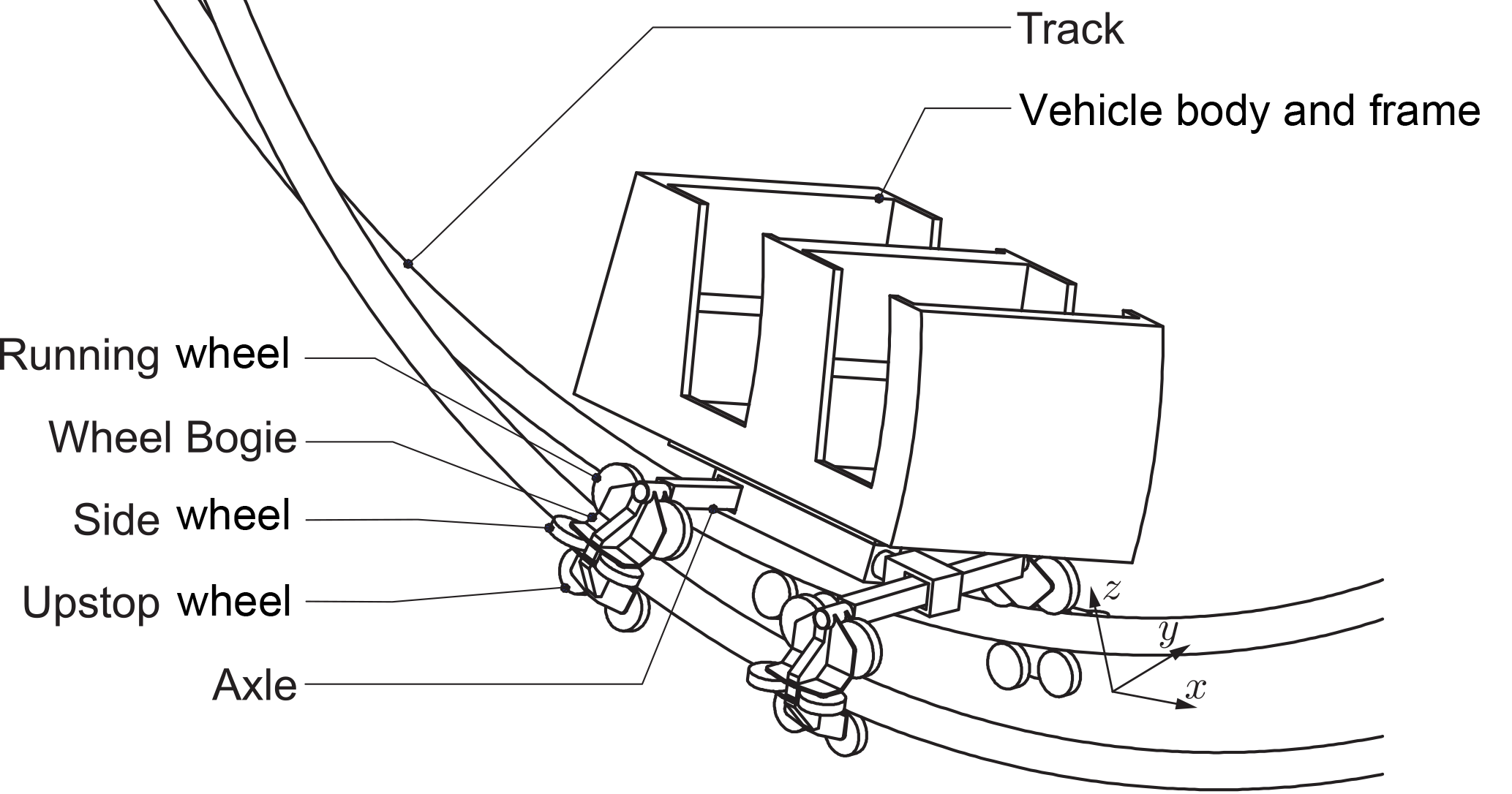
A roller coaster vehicle is usually composed of a vehicle body and frame, which holds the passenger's seat and the restraint system. The wheel bogies are connected to the frame via a central axle or king pins. The concept with an axle is shown in Fig. 1.
In contrast to railway vehicles, the wheels are cylindrical or concave and the track is usually made out of tubular steel pipes (Schwarzkopf, 1972). Each wheel bogie usually holds at least three different types of wheels. The running wheels carry the main load of the vehicle, whereas the side wheels guide the vehicle on the track. The upstop wheels keep the vehicle on the track during negative vertical accelerations. Variations of this similar set-up have been in use since a first vehicle concept like this was patented in the 1920s (Miller, 1921).
2.2 Measurement of wheel forces
Since all forces and moments resulting from the vehicle's motion are transferred from the wheel to the track, the measurement of these is of special interest. On the one hand, they can be used to assess the vehicle dynamics; on the other hand, the loads for the vehicle and the track can be determined. Therefore, different measurement methods have been developed and are currently in use for cars and commercial and rail vehicles. Most of these methods are based on two fundamental force measurement principles, namely the use of strain gauges and a deformation element or piezoelectric force transducers (Weiblen and Hofmann, 1998; Weiler, 1993). Representative applications for both principles are briefly presented here.
A commonly used measurement device for the wheel forces of cars is a dynamometer consisting of a rectangular array comprising four triaxial piezoelectric force transducers (Evers et al., 2002) – Fig. 2.
This arrangement provides 12 force signals which can be used to calculate the normal force and the two tangential forces at the contact point as well as the three moments acting on the wheel. Piezoelectric transducers are characterised by their high linearity and ratio between range and response threshold as well as low cross-talk and hysteresis. Despite these advantages, the cost of the sensors is high and the sensor array needs a designated space, which makes it difficult to fit into small wheels (Bonfig, 1995).
A different type of piezoelectric measurement wheel is presented in Bastiaan (2018). Here piezoelectric strain sensors are incorporated into the rubber tire. Neural networks are employed to determine the relationship between the strain measurement and the wheel forces and moments. However, the estimation is not very accurate.
Other transducers use a deformation element and strain gauges as described in Hufnagel (2000), Späth (2001), Gobbi et al. (2005), Barnett et al. (2014) and Feng et al. (2015).
Rail vehicles usually also employ strain gauges fitted onto the front and backside of the wheel discs of a wheelset as described in Schwabe and Berg (2007), Magel et al. (2008) and Joch et al. (2012). The normal and the tangential force cause strain at the measurement points which depends on their magnitude, the location of the contact point and the wheel radius. A weighted summation of the strain signals is then used to determine the corresponding forces. The waviness of the signal due to the wheelset rotation has to be corrected by low-pass filtering.
Apart from this solution, there exist stationary measuring devices as described in Stephanides et al. (2008) as well. Here, a deformation element equipped with strain gauges is installed at certain locations of the railway track that measures the wheel-rail forces, when the train passes over it.
2.3 Calibration of multi-axis force and torque transducers
The calibration provides the relationship between the p signals of the measurement points (e.g. the bridge voltage of strain gauges, or the electric charge of a piezoelectric element), arranged in the vector u, and the n acting forces and moments on the transducer, arranged in the vector k. It is clear that p needs to be greater than or equal to n in order to determine all components. The relationship can be expressed according to Weiler (1993) as follows:
or
The measurement matrix comprises the matrix with the coefficients for the linear elements uj and with the coefficient for the quadratic and mixed elements uk⋅ul (k≠l). For an n-component transducer with p measuring points, the number of coefficients can be reduced by utilising the commutativity of the multiplication and is shown in Table 1.
Table 1Number of coefficients for an n-component transducer with p measuring points (Giesecke, 2007).
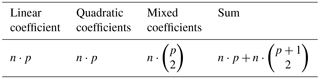
It is obvious that the number of coefficients increases when n and p increase. The required calibration tests are at least the given values in Table 1 divided by p. It is not possible to determine all coefficients uniquely if p>n. If the deformation element is stiff, the quadratic and mixed coefficients are relatively small, and for standard industrial applications they can be neglected (Giesecke, 2007). Equation (2) then simplifies to Eq. (3) and up,1 only contains the linear elements of the measuring signals.
The highest possible rank of Qn,p is n; therefore, the transducer needs to be calibrated with at least m=n linear independent load situations, which yields the following equation:
Matrix Kn,m contains the applied forces and moments measured by a reference transducer; Up,m contains the signals of the measuring points. The unknown measurement matrix Qn,p can be determined by a right-hand multiplication with the Moore–Penrose inverse of Up,m. If p>n, the solution is determined by a least square fit (Knabner and Barth, 2013); for p=n it is unique.
Generally, it is desirable that most of the elements of Qn,p are equal to zero, which can be achieved by a mechanical isolation of the measuring points. This means that a force along one axis only produces a signal at one of the measuring points. The global deviations due to the summation of the signals are less, when only one signal is required to calculate the corresponding force (Giesecke, 2007).
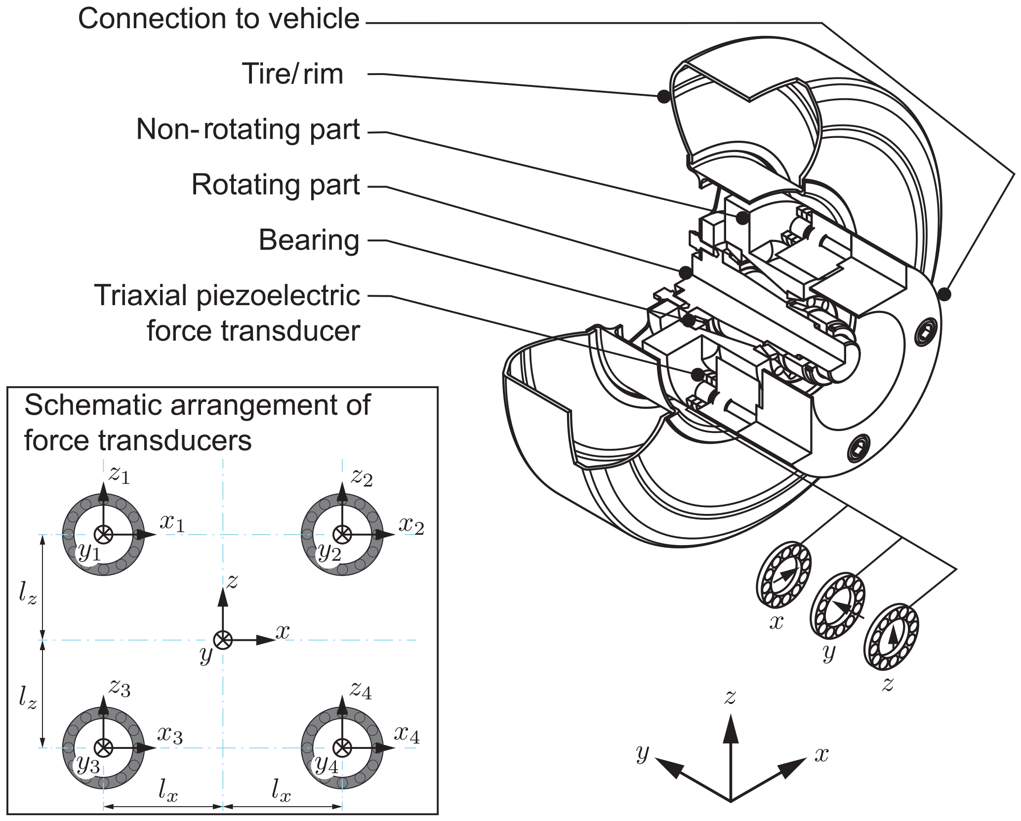
Figure 2Non-rotating dynamometer for a car tire according to Evers et al. (2002) and Bonfig (1995).
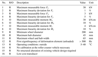
The main focus of the transducer lies on the measurement of the normal force Fz and the tangential force Fy, independent of the contact point location. The transducer needs to fit into the available space of a roller coaster wheel and should easily replace an existing wheel without the need to modify the adjacent parts. The measurement of the moments Mx and Mz is desirable but not essential. It is especially important that the manufacturing costs are low, since a standard roller coaster car can consist of up to four wheel bogies with each holding up to six wheels. Thus at least six transducers are required to measure all forces acting on one wheel bogie. The major transducer specifications, sorted into required (R) and optional (O), are summed up in Table 2.
4.1 Concept
Out of the aforementioned requirements, the most critical constraints for the transducer are the available space in a roller coaster wheel (diameter 200 mm) in conjunction with the maximum normal force of 30 kN and the relatively low manufacturing costs. The space constraint makes it nearly impossible to fit a telemetry system and a power supply for the transducer rotating with the wheel itself. However, all roller coaster wheels have one advantage in comparison to most other vehicle wheels: they spin freely and do not need to transmit longitudinal forces onto the rails. Therefore, the transducer can be fixed to the wheel suspension and the wheel bandage rotates around it, as shown in Fig. 3. The desired manufacturing costs practically prohibit the use of triaxial piezoelectric transducers, since the cost of an array is about EUR 20 000. Therefore a solution using strain gauges is developed.
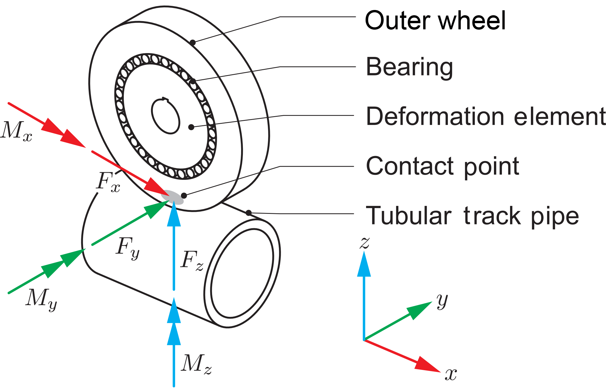
The ring-shaped space for the deformation element is determined by the bearing with an inner diameter of 140 mm. Since the contact point can shift, especially in the y direction, it makes sense to base the transducer on the measurement of shear stresses. The shear force in a beam is constant if no other force is applied on it and it is independent of its lever arm (Giesecke, 2007). In order to create shear forces in the deformation element when a force Fy or Fz is present at the contact point (see Fig. 3), the measurement beams for the shear strain must be aligned in the x direction. To increase the eigenfrequency of the element, a design with four beams is chosen, which is similar to a dynamometer (Fig. 2). Figure 4 shows this configuration, including all acting forces and moments at the contact point.
If the four beams were pin-jointed, no moments would be acting along the measurement beams B1–B4. Then the force and moment equilibriums are
By measuring the eight shear forces By and Bz, it is obviously possible to calculate the forces Fy and Fz as well as the moments Mx and Mz because they are independent of the non-measured normal forces Bx. Fx and My would require the measurement of these normal forces in the beam. However, the wheel spins freely, so these are small and for this application not of interest. In order to withstand the maximum normal force Fz of 30 kN and to minimise hysteresis, an integrated design for the deformation element is chosen. To maximise the shear strains in the four beams, their sections are designed similarly to an I-beam according to the recommendations in Giesecke (2007).

4.2 Modelling
The CAD model of the deformation element with the locations of the strain gauges, each holding two 45∘ patterns, is shown in Fig. 5.
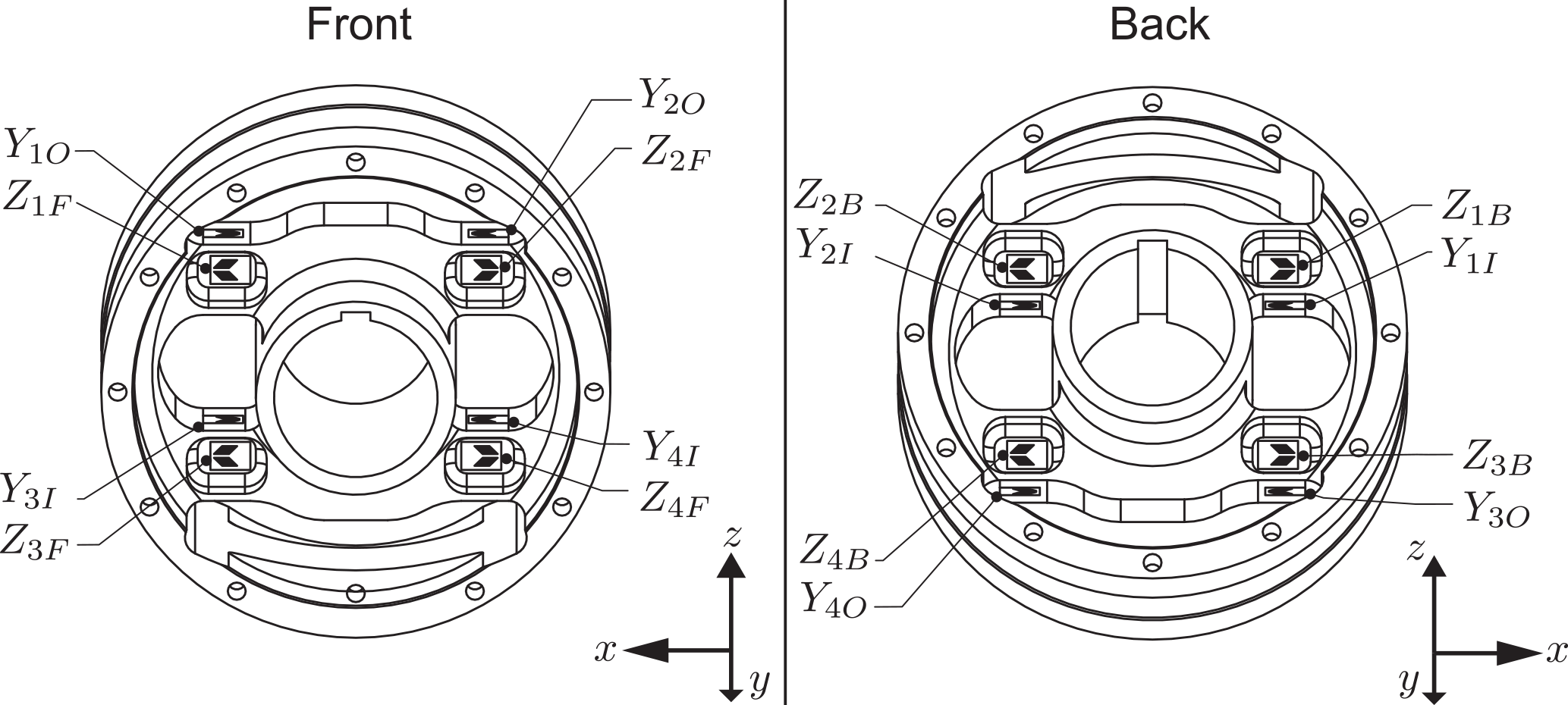
Each of the corresponding strain gauges indexed with F (front)/B (back) and O (outside)/I (inside) are connected to a full bridge to measure eight shear strains. Disturbance forces and moments as well as the temperature strains are compensated by the connection of the bridges (Giesecke, 2007). To analyse the design of the element, a finite element analysis with ANSYS is performed. Figure 6 shows the results when a force Fy or a force Fz, acting along the depicted coordinate axis, is centrally applied at the contact point of the wheel. It can be observed that the measuring points are mechanically isolated. They show only a shear stress if the corresponding force is applied; i.e. if the force Fy is acting, only the gauges Y show a shear strain in the corresponding plane. If Fz is acting, only the gauges Z measure a shear strain. However, if the contact point is laterally shifted, a force Fz will also cause shear stresses for the gauges Y. This is obvious, because a moment Mx is present, which creates a shear force according to Eq. (8). A shift of Fy in the x direction produces a moment Mz and therefore only shear strains at Y. Overall it can be observed that the force Fz can be calculated by using only the signals of the gauges Z (similar to Eq. 7). The force Fy as well as the moments Mx and Mz require a different combination of the signals of the gauges Y for their calculation (Eqs. 6, 8 and 10). Therefore, even with a shift of the contact point, the force Fz is mechanically isolated transmitted to the measuring points from all other acting forces and moments.
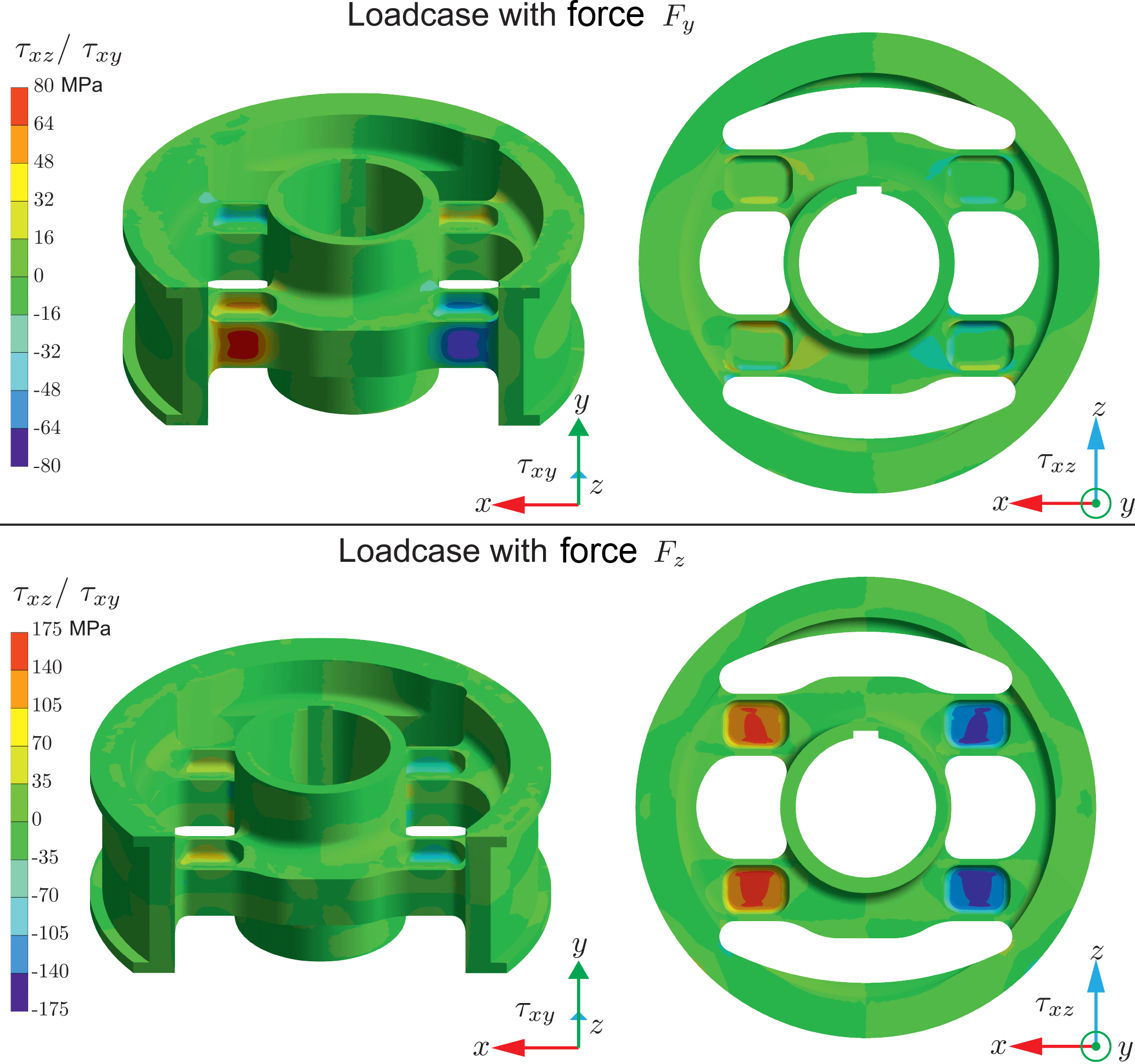
By changing the dimensions of the web of the I-beam profile, the resulting strains for the force Fz can be easily scaled to an optimum value of 1000 µm m−1 (according to Hottinger Baldwin Messtechnik GmbH, 2008) with a small impact on the static strength of the element. Since the expected magnitude of the force Fy is only one-tenth of the force Fz, the corresponding strain is by its nature considerably lower and only 300 µm m−1 for gauges Y3 and Y4 and 160 µm m−1 for Y1 and Y2, respectively. The strain could be increased by reducing the thickness of the I-beam flange. However, since this directly influences the static strength considered for the case when the force Fz is applied, the size reduction is limited.
Furthermore, the FE analysis shows that the first eigenfrequency of the deformation element with no load is above 1200 Hz.
The full design of a measurement wheel with a diameter of 360 mm is shown in Fig. 7. The deformation element with the strain gauges in Fig. 7 is oriented in the same relation to the coordinate system as shown in Fig. 5.
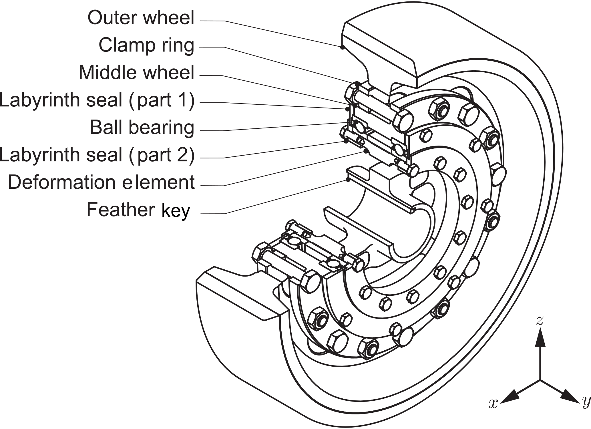
The outer wheel consists of an aluminium rim with a vulcanised polyurethane bandage. It is fixed with a ring onto the middle wheel that holds the bearings, so that the outer wheel can be easily replaced. The bearings in O-arrangement are contactless sealed with a self-made labyrinth seal to minimise friction. The inner ring of the bearing is fitted onto the deformation element with the strain gauges. To prevent its rotation, a feather key is present on the upper, load-free side of the wheel hub. The same deformation element can be used used for a 200 mm diameter wheel with a thin section bearing.
In order to determine the measurement matrix according to Sect. 2.3, two basic methods are available. The first one is a theoretical calibration by using a finite element analysis and the second one is an experimental calibration with an actual test rig and reference force transducers.
5.1 Theoretical calibration
For the theoretical calibration, the geometry of the deformation element without the other parts of the wheel is analysed with a finite element analysis using different load cases to determine the average strains acting on the area of the strain gauges. The main advantage of this method is that no actual manufactured parts as well as a calibration test rig are required. Also, the geometry and the load application are ideal. Thus this method describes the best possible conditions.
As described in Sect. 4 there are p=8 measuring points for n=4 force and moment components. Therefore, the measurement matrix is rectangular and at least eight different load cases would be required to determine all coefficients. However, there are only n=6 force and moment components available which can act on the transducer. Thus, the resulting system of equations is under-determined and the solutions for the measurement matrix are infinite. Furthermore, a calibration with the disturbance forces Fx and My is required. According to Sect. 2.3 there are only measuring points required to measure n=4 components Fy, Fz, Mx and Mz. By employing the relationships of Eqs. (6), (7), (8) and (10), the signals of the measuring points can be reduced to
This formula uses the symmetries of the deformation element and for the calibration only the measurable components Fy, Fz, Mx and Mz must be used. It must be noted that the proposed signal reduction in Eq. (11) cannot be realised completely electrically – only the summation of the signals Z is possible by a parallel or antiparallel connection of the strain gauge's bridge and supply voltages.
The measurement matrix Q4,4, given in Eq. (12), is calculated out of four different load cases with the finite element analysis. The rows are labelled with the component that is calculated with the sum of the corresponding column elements multiplied by the signals of u4,1, which are indicated at the column locations.
The absolute values of only six coefficients are significantly larger than zero. Again, the mechanical isolation of the measuring points Z regarding Fz can be observed, since the last column shows only one coefficient substantially larger than zero. As expected by Eqs. (6), (8) and (10), the measuring points Y are not mechanically isolated regarding the measurement of the force Fy. They show a signal when the force Fy or a moment Mz caused by Fy or a moment Mx caused by a y shift of the force application point of Fz is present. By using the matrix, the deformation element can be tested with different load cases, load application points and disturbance forces. In all load cases, the forces at the contact point can be measured with deviations less than 0.0001 %, the moments with 0.05 % compared to the nominal value. This means that even under ideal conditions, there are deviations. The reasons for these are the distortion of the deformation element and the resulting change in the lever arms as well as a non-symmetric finite element grid.
5.2 Experimental calibration
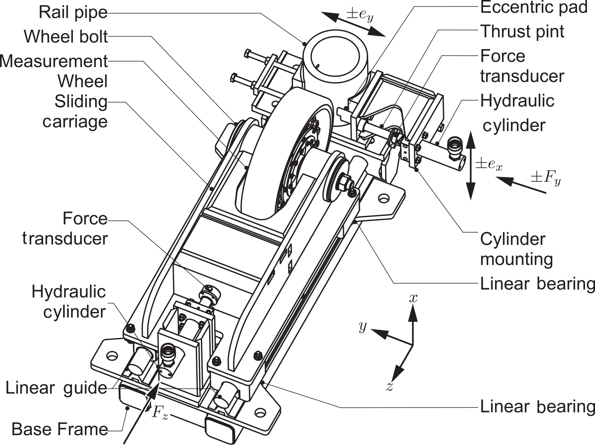
The mechanical properties of the deformation element, its manufacturing, and the positioning of the strain gauges are always subject to certain tolerances. Therefore, an experimental calibration is necessary. This is carried out with a specially designed calibration rig as shown in Fig. 8 that allows a static calibration. It basically consists of a sliding carriage on linear guides and a rail pipe console that can be shifted in the y direction. The measurement wheel is installed on the sliding carriage and the deformation element is oriented in the same relation to the coordinate system as shown in Fig. 7. The force is applied with two hydraulic cylinders and is measured with reference transducers. The moment Mx is applied by shifting the rail pipe console, the moment Mz by shifting the application point of the force Fy. It must be noted that the application of Fz and Mx is close to the actual wheel–rail contact. For Fy and Mz a static calibration cannot provide this. These components occur in the contact area of the cylindrical wheel with the cylindrical rail due to slip, which requires a rolling or sliding contact (Knothe and Stichel, 2003). The force Fy is therefore applied with a thrust pin and an eccentric pad over a larger contact area at the side of the wheel so as not to damage the polyurethane bandage.
For each component, apart from the force Fz, several load cases with the maximum value in two directions (positive and negative) are carried out. For Fz, only the positive maximum force is applied, since the wheel has a unilateral contact with the rail. Also, the load is applied under different angular positions, since the turning of the wheel can cause inner stresses on the deformation element. In total 121 load cases are used for the calibration and the measurement matrix is determined with the right multiplication of the Moore–Penrose inverse U in Eq. (4). The experimentally identified measurement matrix is given in Eq. (13).
The overall agreement between the finite element calibration and the experiment is good. As expected, the mechanical and electrical isolation of the measuring points is less distinct. The corresponding coefficients are still close to zero but several times larger than in Eq. (12). The largest deviation to the finite element analysis can be observed at the coefficients for the moments; however, the load application in the calibration rig is based on a distance measurement, which is less accurate. Especially the moment Mz is introduced by a force Fy where the load application point is not very distinct due to the area of the pad.
6.1 Linearity
To assess the linearity deviation, the actual values of the force and moment components, calculated by multiplying the measurement matrix by signals of the strain gauges, are compared to the target value of the reference transducers. If these are plotted together, they should ideally show a straight line through the origin with a slope of 1. The deviations from the ideal measurement are presented in Fig. 9.
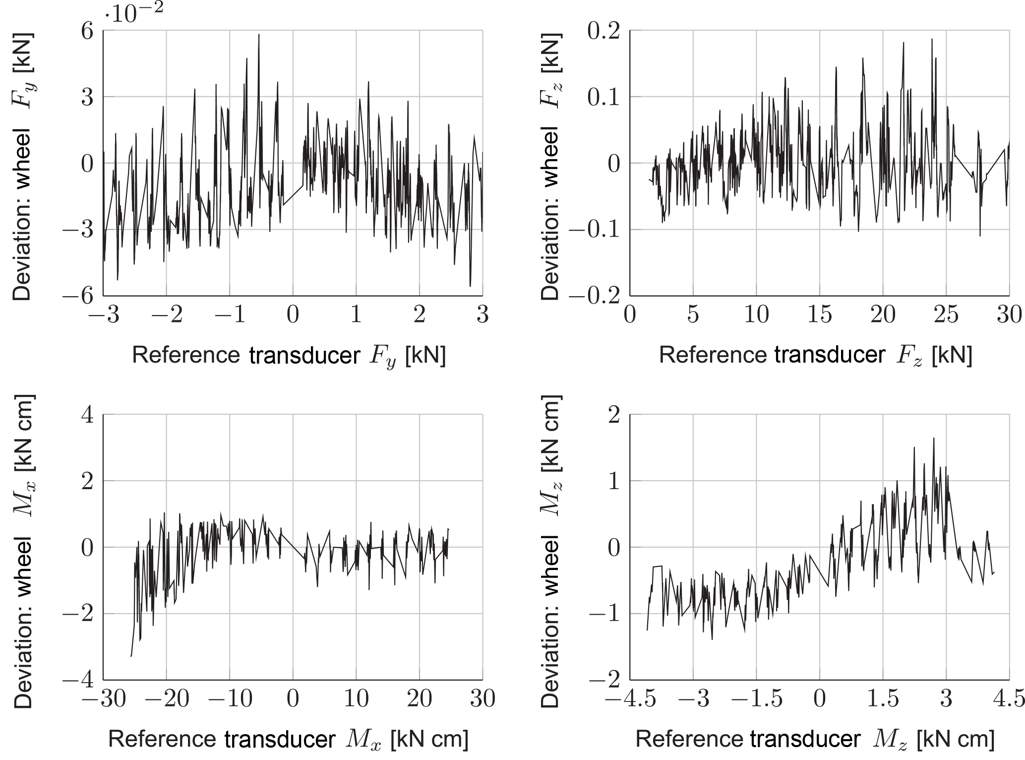
The maximum deviation of the actual to the target values divided by the nominal value is defined as the linearity deviation (Dubbel et al., 1997). Depending on the manufacturing quality of the wheel, the linearity deviations for Fy are less than 2 %, and for Fz less than 0.6 %. These deviations are regarded as good for a non-industrial transducer with an arbitrary force application point. The deviations for the moments are higher, and range between 6 % and 18 % for Mx and between 10 % and 57 % for Mz. The reasons for these deviations are the inner stresses acting on the deformation element when turning the outer wheel. They cause a shift of the zero point for all strain gauge signals. This shift is only compensated for the force Fy and Fz, because they are calculated by an unweighted sum (refer to Eqs. 6 and 7). For the moments the sum must be weighted (refer to Eqs. 8 and 10), and so the zero shift cannot be compensated. This disturbance can be reduced if the manufacturing of the press fit for the bearing has smaller tolerances. Besides, a heat treatment of the deformation element can reduce stresses due to machining. Since the disturbance is generated by turning the wheel, a low-pass filtering can also reduce this. However, the usable frequency range of the transducer decreases, respectively.
6.2 Normally distributed deviations
To get a more global view of the deviations and to incorporate effects of the cross-talking, the deviations can also be treated as normally distributed (Parthier, 2008). To prove this, the difference between the actual and target values are calculated for all load cases and sorted according to their value and relative quantity. This creates a histogram as shown in Fig. 10. For all deviations the mean value and the standard deviation are calculated and the corresponding normal distribution is also shown in Fig. 10.
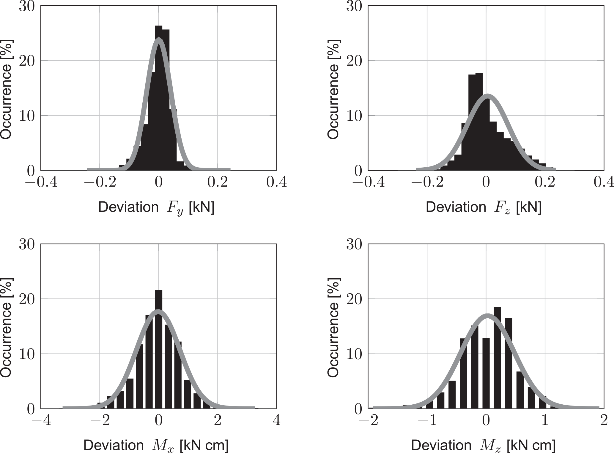
It can be observed that they are approximately normally distributed; thus, an interval with the positive and negative limits twice the standard deviation holds 95.5 % of all deviations (Parthier, 2008). These limits in relation to the nominal value are herein defined as normally distributed deviations. For Fy they are less than 2 % and for Fz less than 0.5 %, depending on the manufacturing quality. These values are similar to the linearity deviations. The measurement of the moments again shows higher deviations which are between 3 % and 11 % for Mx and between 5 % and 36 % for Mz, being slightly lower than the linearity deviation. Overall, it can be stated that the forces can be measured with low and acceptable deviations. The measurement of the moments has an orientating character if they are not filtered.
7.1 Reproducibility of the measurement results
The four manufactured measurement wheels are installed in a wheel bogie of an existing roller coaster train as running and side wheels (Fig. 1). Furthermore, the position of the train is captured by counting the rotations of the wheel. Several runs are carried out under similar conditions. However, it must be noted that the velocity of the train varies on each run since it is influenced by a lot of parameters, such as the temperature of all bearings and the wheel bandage as well as the current wind and weather situation. A variation of the velocity v significantly changes the load on the wheels. Its influence is quadratic since e.g. the centrifugal acceleration a of a body following a circular path with radius r is calculated according to Dankert and Dankert (2011):
To determine the random deviation, the concepts of the DIN 1319-1 (1995) are employed; i.e. a fictive mean measurement is created out of five measurements by calculating the mean value of each measurement on each synchronised waypoint. The deviations to this mean measurement are calculated for all five measurements on each waypoint. Lastly, out of all deviations the standard deviation in relation to the nominal values (given in Sect. 3) is determined as shown in Fig. 11.

Figure 11Standard deviation for five unfiltered measurements from a fictive mean value measurement: Fy, Fz, Mx, Mz.
The standard deviations are similar to the previously discussed normally distributed deviations (Sect. 6.2), so only the forces can be measured with an acceptable deviation.
As previously stated, the deviations of the moments are a result of inner stresses that shift the zero point if the wheel is turned. Thus, they can be reduced if the data are low-pass filtered, which is achieved here with a moving average filter with a width of 200 ms. The random deviations decrease significantly, as shown by their standard deviation in relation to the nominal value – Fig. 12. Thus, by sacrificing the dynamic range of the transducer, even the moments can be measured with an acceptable random deviation. In addition, the remaining deviations are actually not random: they are caused by the change in the velocity of the train.
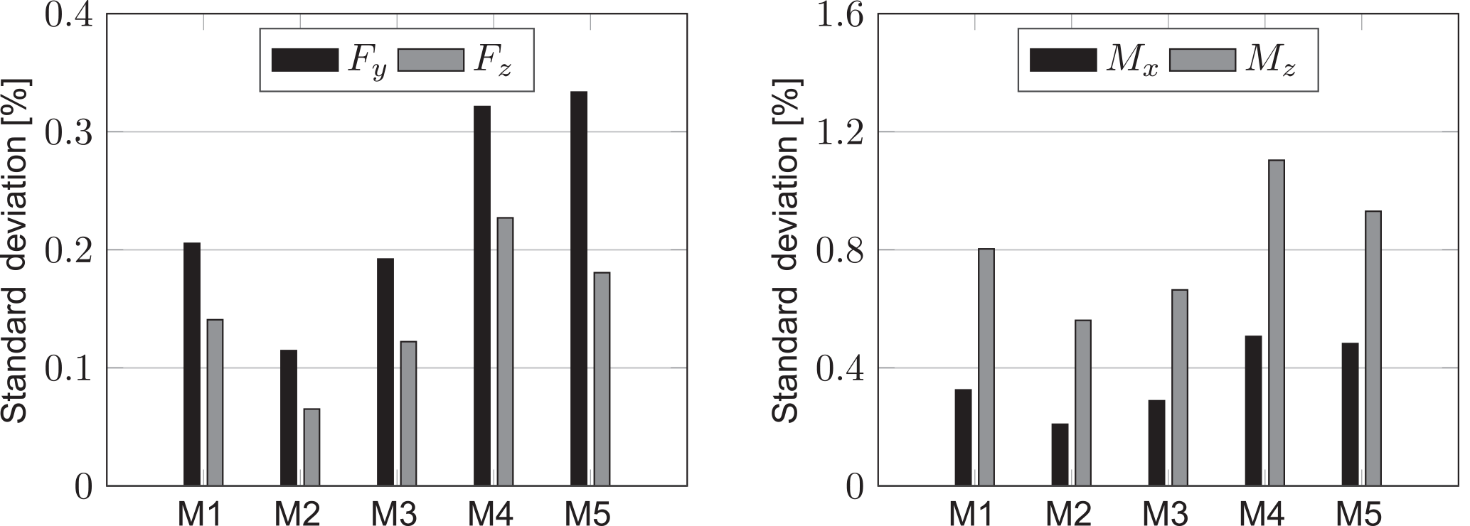
Figure 12Standard deviation for five filtered measurements from a fictive mean value measurement: Fy, Fz, Mx, Mz, moving average filter with 200 ms width.
7.2 Results and comparison to simulations
To evaluate the measurements, they are compared to the results of a multibody simulation (MBS) of the roller coaster train on the same track. The MBS was carried out with SIMPACK employing the FASTIM algorithm (Kalker, 1982) for the calculation of the tangential forces and material parameters for viscoelastic wheels according to Knothe and Miedler (1995). It must be noted that in the MBS an ideal track geometry without any disturbances is simulated. To dampen disturbance from the track position, the measurements are filtered with the above-mentioned moving average filter and compared to the simulated values. Representatively, Figs. 13 and 14 show the results of the simulation and the measurement for the tangential force Fy on a side wheel and normal forces Fz on a running wheel.
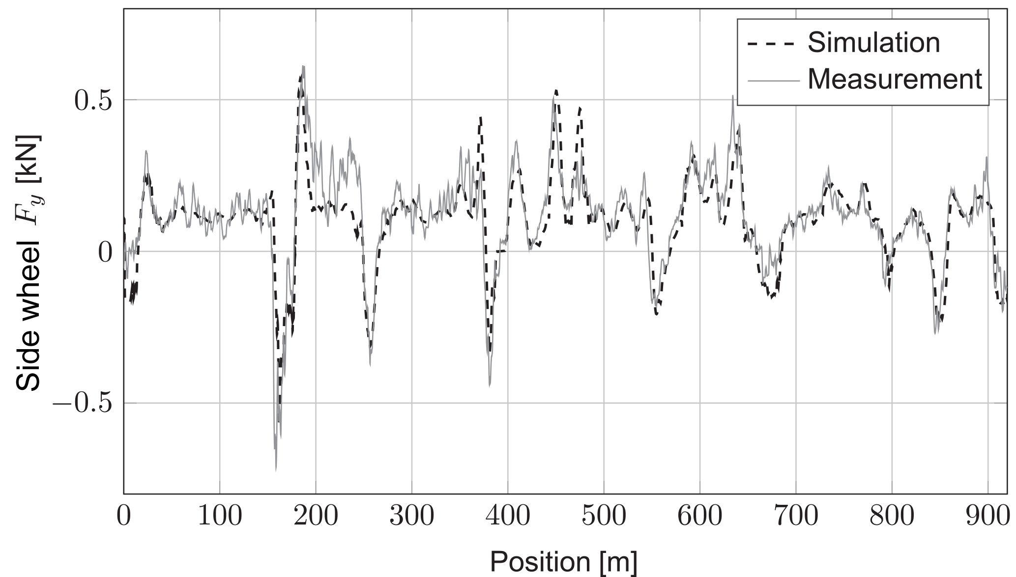

The overall agreement is good and it is especially remarkable that the FASTSIM algorithm predicts the tangential forces due to slip very well even for viscoelastic wheels that are treated herein as purely elastic. However, it must be noted that according to Braat (1993), viscoelastic effects in rolling contact are less signficant for the relevant high velocities in roller coaster applications (). Furthermore, the force mostly depends on the track geometry and the resulting slip angle of the wheels, which is underlined by the high reproducibility as described in Sect. 7.1.
The normal forces on the wheel are also mostly generated by the track geometry itself. They represent the main loads on the wheel. As can be observed in Fig. 14 the agreement is also good. From positions 0 to 550 m the wheel loads of the measurement are higher than the simulated ones. However, the simulated velocity is also higher than the measured ones, so part of the deviations can be explained by that fact (see also Eq. 14). For the rest of the ride the simulated velocity matches the measured one closely (deviations less than 0.2 m s−1). Therefore, the simulated wheel load is closer to the measured one. Also, it is easy to identify the track areas where the upstop wheel is in contact with the track pipe. These are the waypoints 15, 175, 675 and 915 m, because the measured and simulated wheel forces are close to 0 kN (i.e. <0.2 kN). It must be noted that even the unfiltered measurements show these areas. This emphasises the fact that even if the wheel is turning at high speed the zero shift due to inner stresses is compensated by the arrangement and interconnection of the strain gauges. No force is measured if no force is present, even if the wheel spins fast.
By comparing the normal force Fz of the running wheel (Fig. 14) with the tangential force Fy of a side wheel (Fig. 13), it can be observed that Fy is negative when Fz is lower than the resulting force due to the dead weight of the vehicle (approx. 5 kN). This can be easily explained, since the side wheel is perpendicularly mounted to the running wheel (Fig. 1). If the normal force Fz of the running wheel is lower than the force due to the vehicle's dead weight, the wheel suspension of the running wheel rebounds and the wheel bogie with the side wheel moves in the z direction (Fig. 1). This movement creates a slip velocity along the local y axis of the wheel (Fig. 7) which results in a tangential force Fy on the wheel.
The article proposes a simple and low-priced design for a force and torque transducer incorporated into an non-driven wheel with an outer diameter as small as 200 mm while still being able to carry and measure a maximum normal force of 30 kN. Also, it is possible to measure tangential forces in the axial direction, which are only one-tenth of the normal force. Furthermore, the application point of the forces does not need to be specified exactly. The design is easily scalable to measure different forces and can be used for all kinds of non-driven wheels.
By performing a theoretical calibration, the best possible results of the developed transducer under ideal conditions were shown. The experimental calibration showed higher deviation to the reference, but for measuring the forces these were still comparatively low (less than 2 % of the nominal value). Due to manufacturing tolerances of the transducer, the measurement of the moments acting on the wheel has only an orientating character. It can be dramatically improved by low-pass filtering the data; however, this reduces the frequency range of the transducer. Therefore, further studies should focus on improving the manufacturing quality and eliminating the zero shift that results from turning the wheel. Especially improving the circularity or changing the fit of the bearing seat could reduce these deviations significantly. One should investigate whether it is possible to measure the moments with acceptable deviations.
By employing the measurement wheel in a roller coaster vehicle, the real-life application of the transducer design was successfully demonstrated. The comparison to a multibody simulation under similar conditions showed a good agreement. Therefore, the proposed design can be used to assess the loads acting on a roller coaster wheel and thus also acting on the rail, its support structure and the adjacent vehicle frame. Furthermore, it could be possible to use the designed wheel not only for the purpose of validating the load assumptions, but also to integrate it permanently into the roller coaster vehicle. Then it would be possible to monitor the condition of the vehicle and track during operation. The wheel could communicate with the control system and the system could react as described in Hauer (2015).
The measured data are not publicly available. They were only used as an example to show the capability of the developed transducer. The data are not necessary to develop or reproduce a similar transducer, which is the main focus of the article.
AS developed the transducer, performed the calibration as well as the experiments and wrote the article; CS reviewed and provided corrections for the article.
Andreas Simonis was previously employed by Gerstlauer Amusement Rides GmbH and plans to work henceforth. However, he would like to state that his work was not influenced by this employment.
The authors would like to thank Gerstlauer Amusement Rides GmbH for their
support.
Edited by: Bernhard
Jakoby
Reviewed by: three anonymous referees
ASTM F2137-16: Standard Practice for Standard Practice for Measuring the Dynamic Characteristics of Amusement Rides and Devices, available at: https://www.astm.org/Standards/F2137.htm (last access: 1 September 2018), 2016. a
Barnett, S., Graves, R. G., Leake, G. E., Nelson, B. J., Boram, A. J., Benetti-Longhine, L. R., and Walter, J. A.: Wheel force measurement system, Patent US8640553B2, 2014. a
Bastiaan, J. M.: Physical Validation Testing of a Smart Tire Prototype for Estimation of Tire Forces, SAE Technical Paper Series, SAE International400 Commonwealth Drive, Warrendale, PA, United States, https://doi.org/10.4271/2018-01-1117, 2018. a
Bonfig, K. W.: Technische Druck- und Kraftmessung: Mit 3 Tabellen, vol. 254, Mess- und Prüftechnik of Kontakt & Studium, Expert-Verl., Renningen-Malmsheim, 2. edn., 1995. a, b
Braat, G. F.: Theory and Experiments on Layered, Viscoelastic Cylinders in Rolling Contact, Dissertation, TU Delft, Delft, 1993. a
Braccesi, C., Cianetti, F., and Landi, L.: Integrated Roller Coaster Design Environment: Dynamic and Structural Vehicle Analysis, in: ASME 2015 International Mechanical Engineering Congress and Exposition, V04BT04A004, https://doi.org/10.1115/IMECE2015-51504, 2015. a
Dankert, J. and Dankert, H.: Technische Mechanik: Statik, Festigkeitslehre, Kinematik/Kinetik; mit 128 Übungsaufgaben, zahlreichen Beispielen und weiteren Aufgaben im Internet, Studium, Vieweg + Teubner, Wiesbaden, 6. edn., 2011. a
DIN 1319-1: Grundlagen der Messtechnik – Teil 1: Grundbegriffe, 1995. a
Dubbel, H., Beitz, W., and Grote, K.-H.: Taschenbuch für den Maschinenbau – Dubbel, Springer, Berlin, 19. edn., 1997. a
Evers, W., Reichel, J., Eisenkolb, R., and Ebhart, I.: RoaDyn™ – Ein Entwicklungswerkzeug für Felge und Radaufhängung, available at: https://www.fzd.tu-darmstadt.de/media/fachgebiet_fzd/publikationen_3/2002/2002_eversreicheleisenkolbebhart_kistler.pdf (last access: 1 September 2018), 2002. a, b
Feng, L., Lin, G., Zhang, W., Pang, H., and Wang, T.: Design and optimization of a self-decoupled six-axis wheel force transducer for a heavy truck, P. I. Mech. Eng. D.-J. Aut., 229, 1585–1610, https://doi.org/10.1177/0954407014566439, 2015. a
Giesecke, P.: Mehrkomponentenaufnehmer und andere Smart Sensors: Der mechatronische Ansatz in der DMS-Technik, vol. 75 of Edition expertsoft, Expert-Verl., Renningen, 1. edn., 2007. a, b, c, d, e, f
Gobbi, M., Aiolfi, M., Pennati, M., Previati, G., Levi, F., Ribaldone, M., and Mastinu, G.: Measurement of the forces and moments acting on farm tractor pneumatic tyres, Vehicle Syst. Dyn., 43, 412–433, https://doi.org/10.1080/00423110500140963, 2005. a
Hauer, R.: Vorrichtung und Verfahren zur Erhöhung der Sicherheit von Achterbahnen und/oder Karussells, Patent DE102015102556A1, 2015. a
Hottinger Baldwin Messtechnik GmbH: Der Weg zum Messgrößenaufnehmer: Ein Leitfaden zur Anwendung der HBM K-Dehnungsmessstreifen und Zubehör, available at: https://www.hbm.com/de/3736/tips-tricks-aufnehmerbau/ (1 September 2018), 2008. a
Hufnagel, K.: Internal- and Half-Model Balances built at the Wind Tunnel Facility of TUD, available at: https://www.sla.tu-darmstadt.de/media/fachgebiet_sla/windkanal_sla/produkte_sla/Balance-Brochure.pdf (last access: 1 September 2018), 2000. a
Joch, M., Mader, P., and Hutterer, H.: Messradsatz für Schienenfahrzeuge, Patent EP2439508A1, 2012. a
Kalker, J. J.: A Fast Algorithm for the Simplified Theory of Rolling Contact, Vehicle Syst. Dyn., 11, 1–13, https://doi.org/10.1080/00423118208968684, 1982. a
Knabner, P. and Barth, W.: Lineare Algebra, Springer-Verlag, Berlin, Heidelberg, https://doi.org/10.1007/978-3-642-32186-3, 2013. a
Knothe, K. and Miedler, U.: Analytische Näherungsformeln für den Rollwiderstand elastischer und viskoelastischer Walzen, Konstruktion, 47, 118–124, 1995. a
Knothe, K. and Stichel, S.: Schienenfahrzeugdynamik, Springer, Berlin, 2003. a
Magel, E., Tajaddini, A., Trosino, M., and Kalousek, J.: Traction, forces, wheel climb and damage in high-speed railway operations, Wear, 265, 1446–1451, https://doi.org/10.1016/j.wear.2008.01.036, 2008. a
Miller, J. A.: Pleasure-Railway Structure, Patent US1373754A, 1921. a
Parthier, R.: Messtechnik: Grundlagen und Anwendungen der elektrischen Messtechnik für alle technischen Fachrichtungen und Wirtschaftsingenieure, Vieweg Verlag, Wiesbaden, 4. edn., 2008. a, b
Pfeiffer, F.: Dynamics of Roller Coasters, in: ASME 2005 International Design Engineering Technical Conferences and Computers and Information in Engineering Conference, 413–421, https://doi.org/10.1115/DETC2005-84093, 2005. a
Pombo, J. and Ambrosio, J.: Modelling tracks for roller coaster dynamics, Int. J. Vehicle Des., 45, 470–500, https://doi.org/10.1504/IJVD.2007.014916, 2007. a
Schwabe, O. and Berg, H.: Messradsatz für Schienenfahrzeuge, Patent EP1780524A2, 2007. a
Schwarzkopf, A.: Gleiskonstruktion für eine Belustigungsvorrichtung, Patent DE1703917A, 1972. a
Späth, R.: Messrad für die Erfassung der Radkräfte an der Traktorhinterachse, Landtechnik, 56, 312–313, 2001. a
Stephanides, J., Maicz, D., and Weilinger, W.: Verfahren und Vorrichtung zur Erfassung der Entgleisungsgefahr von Schienenfahrzeugen, Patent WO2007009132 A3, 2008. a
Tändl, M.: Dynamic simulation and design of roller coaster motion, vol. Nr. 423 of Fortschritt-Berichte VDI/20, VDI-Verl., Düsseldorf, 2009. a
Weiblen, W. and Hofmann, T.: Evaluation of Different Designs of Wheel Force Transducers, SAE Technical Paper Series, SAE International400 Commonwealth Drive, Warrendale, PA, United States, https://doi.org/10.4271/980262, 1998. a
Weiler, W.: Handbuch der physikalisch-technischen Kraftmessung: Mit 22 Tabellen, Praktikerbücher, Vieweg, Braunschweig, 1993. a, b