Multi-parameter sensing using thickness shear mode (TSM) resonators – a feasibility analysis

Multi-parameter sensing is examined for thickness shear mode (TSM) resonators that are in mechanical contact with thin films and half-spaces on both sides. An expression for the frequency-dependent electrical admittance of such a system is derived which delivers insight into the set of material and geometry parameters accessible by measurement. Further analysis addresses to the problem of accuracy of extracted parameters at a given uncertainty of experiment. Crucial quantities are the sensitivities of measurement quantities with respect to the searched parameters determined as the first derivatives by using tentative material and geometry parameters. These sensitivities form a Jacobian matrix which is used for the exemplary study of a system consisting of a TSM resonator of AT-cut quartz coated by a copper layer and a glycerol half-space on top. Resonant and anti-resonant frequencies and bandwidths up to the 16th overtone are evaluated in order to extract the full set of six material–geometry parameters of this system as accurately as possible. One further outcome is that the number of employed measurement values can be extremely reduced when making use of the knowledge of the Jacobian matrix calculated before.

1 Introduction

For many years thickness shear mode (TSM) resonators such as the quartz crystal microbalance (QCM) measuring systems are in use for direct recording of mechanically varying situations on a small geometric scale. The essential part of such devices is a piezoelectric plate with electrodes on both sides, enabling the excitation of thickness shear mode vibrations by applying an alternating current (a.c.) voltage. The configuration implies the occurrence of resonant behavior, i.e., a small frequency range with strongly increased oscillation amplitude at a given applied voltage amplitude. The peak frequency (resonant frequency) is shifted under the influence of changed boundary conditions at the plate surface, such as the case at the deposition of a thin layer or at an impact of an adjacent fluidic (gaseous and liquid) medium on one or both plate surfaces. Just these plausible exemplary situations have been crucial for the first relevant publications on this matter by Sauerbrey (1959) and King Jr. (1964).

The considered configuration of a TSM resonator also includes the appearance of higher harmonics. Thus, the examination of different harmonic resonant frequencies can enlarge the sensing issues of the device (Johannsmann, 2001; Q-Sense E4 Operator Manual, 2010). To an increasing degree, biological configurations are also explored (Li et al., 2005; Eisele et al., 2012; Schönwälder et al., 2014) which are lossy as a rule. For a long time, the widths of resonance peaks have also been used for the mechanical evaluation of a lossy material system under study (Rodahl and Kasemo, 1996; Johannsmann et al., 2009; Oberfrank et al., 2016). A common parameter to describe that bandwidth is the so-called full width at half-maximum (FWHM), given as the difference of frequencies belonging to one-half of the squared maximum of admittance amplitude. Due to the existence of so-called anti-resonant frequencies for piezoelectric plates, i.e., the frequency of minimum admittance amplitude, the bandwidths are influenced not only by the mechanical properties but also by the piezoelectric strength of a TSM plate. We define the FWHM of anti-resonance as the difference of frequencies belonging to one-half of the squared maximum of impedance amplitude.

Obviously, a considerable number of measuring data can be taken from TSM resonator experiments which are worth being examined as a function of mechanical properties of the surroundings of a TSM plate. The approach to monitor more than one changing material parameter has been made by several authors (see, for example, Martin et al., 1991; Lucklum et al., 1999; Johannsmann, 2008), but the aim of this work is to treat the problem in a more general manner.

We extend the procedure of sensing properties to many parameters and search for suitable combinations of experiments in order to achieve accurate results as much as possible. The ability for the design of an optimal experimental strategy is the final goal of our study. The theoretical treatment of that problem is based on non-approximated relations between the experimental quantities, i.e., admittance and impedance vs. frequency, and the material parameters (Weihnacht et al., 2007; Bruenig et al., 2008). With this, the popular way of performing that process in terms of equivalent circuits, as introduced by Butterworth (1915) and Van Dyke (1926) for the first time, will be avoided. Having the mentioned relations, all derivatives of significant frequencies (resonant, anti-resonant frequencies, and FWHM frequencies) with respect to the searched material parameters can be calculated. This will be done on the basis of a set of material parameters assumed to be reasonable. The mentioned derivatives have the character of sensitivities and form a Jacobian matrix.

The determination of uncertainties of extractable parameters from TSM resonator measurements are found in the literature only in exceptional cases (Lucklum et al., 1998). A thorough treatment of that problem for the complex situation of multi-parameter sensing is the content of the final part of this study. It will be carried out in a quite similar manner by using Jacobian matrices as was calculated for surface acoustic waves (SAW) in literature (Kovacs et al., 1988; Weihnacht et al., 2017).

The general aim of the present study is consistent with accentuation formulated in current literature (see, for example, Rupitsch, 2019): “simulation-based material characterization” is “of great interest to science and industry”.

2 Electromechanical behavior of TSM resonators

In view of the complexity of the addressed task, we start with the electromechanical basics of TSM resonators. The configuration of the material system under study is shown in Fig. 1. It consists of a piezoelectric single crystal plate, such as quartz, with electrodes, stacks of layers, and half-spaces on the bottom and on top. According to the TSM concept it is one-dimensional in the direction normal to the interfaces. The application of an a.c. voltage at the electrodes creates frequency-dependent oscillations in the system.

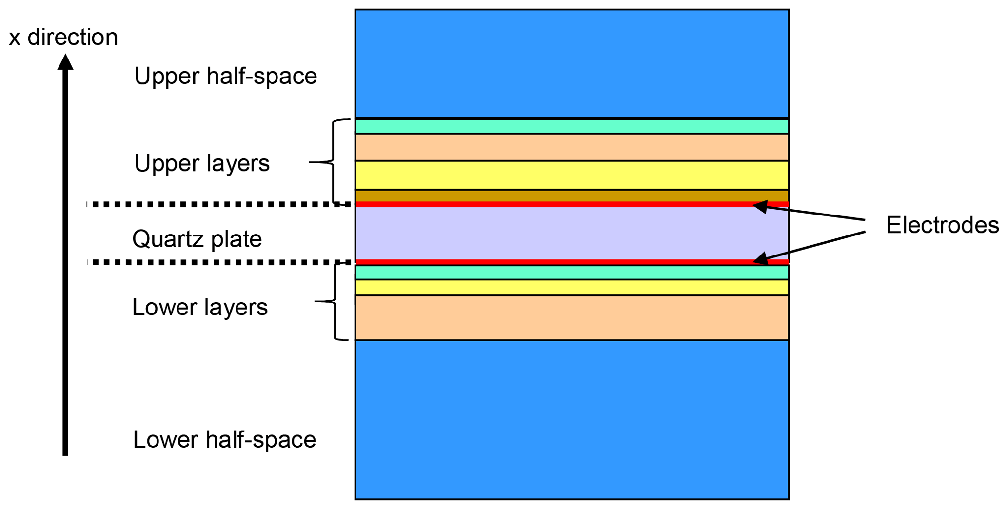
Figure 1 One-dimensional material configuration consisting of a piezoelectric plate, such as quartz, with electrodes, stacks of layers, and half-spaces on both sides.

2.1 Christoffel equation for bulk acoustic wave (BAW) propagation in piezoelectric media

The sensing behavior of TSM resonators is based on the correct mathematical description of the dynamic behavior of the material system of Fig. 1. The one-dimensionality results in a treatment which comprises the propagation of bulk acoustic waves (BAWs) in the direction normal to the surfaces for each part of the material system and the fulfillment of boundary conditions at all interfaces and surfaces. The electromechanical material properties of quartz plate, layers, and of fluidic half-space result in specific BAW parameters in each case. BAW parameters are the phase velocity which can have an imaginary part in lossy materials, besides the particle displacements and the electric potential of wave.

For simplicity we assume isotropic symmetry for the layers and for the half-spaces. We use one more simplification: due to the coverage of quartz plate by electrodes on both sides, the electric potential is constant outside the plate. So we focus the discussion on the more complicated BAW behavior in the quartz plate for now. According to the point group symmetry 32, quartz has six independent elastic stiffness constants (c_ijkl), two piezoelectric coefficients (e_ikl), and two dielectric constants (ε_ij). All these parameters are contained in the following equations which determine the electromechanical behavior of a piezoelectric plate in electrostatic approximation. ρ denotes the mass density, u_i the particle displacement in the i direction, x_i the spatial coordinate of a rectangular system, T_ij the stress tensor, S_kl the strain tensor, D_i the electric displacement, and E_k the electric field. We make use of Einstein's summation convention in all the following expressions.

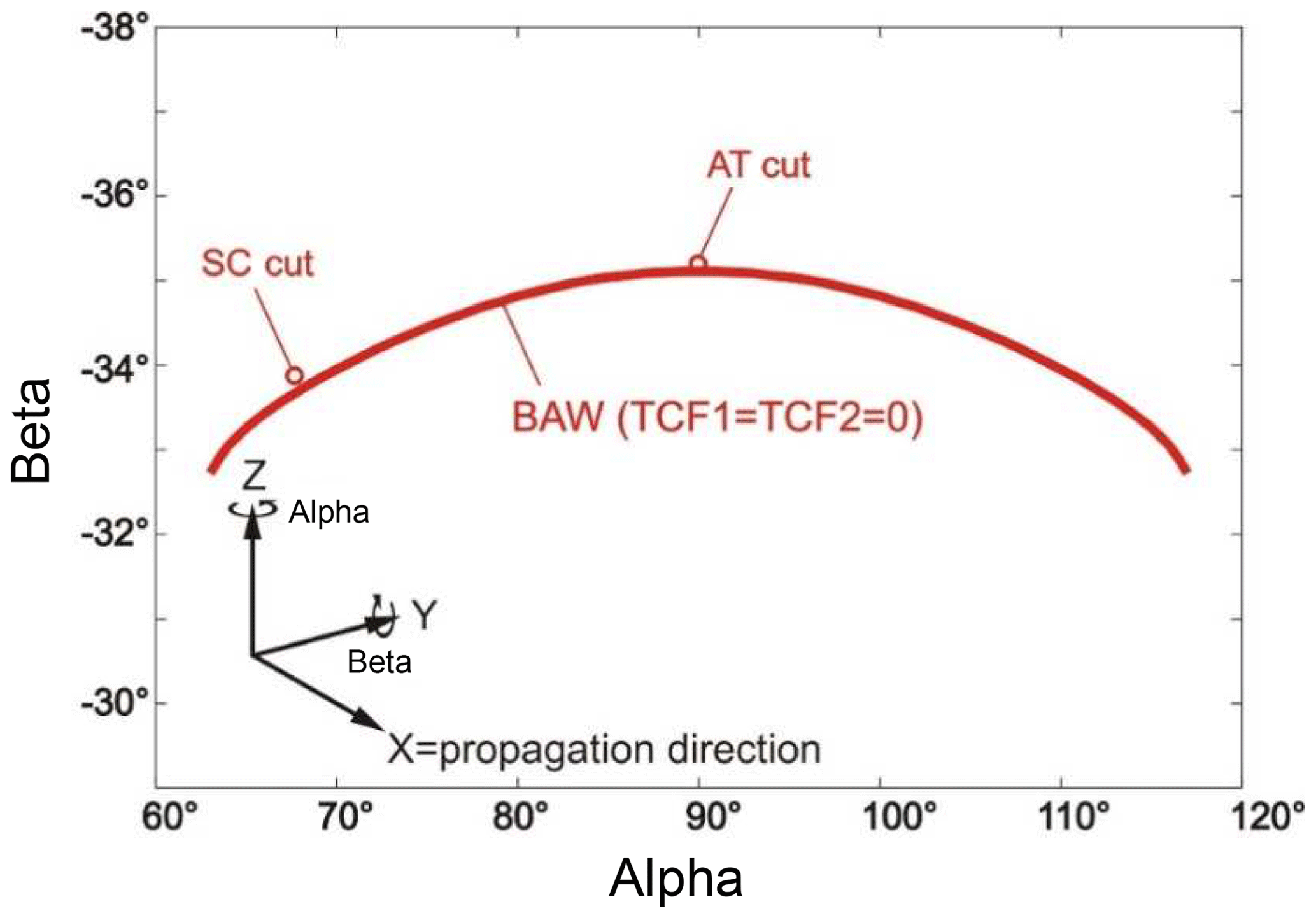
Figure 2 Two preferential orientations of quartz crystals for TSM applications: AT and SC cuts represent directions with small first- and second-order temperature coefficients of frequency constant (TCF). Besides this, the SC cut is stress-insensitive. The initial (x, y, and z) axes form the physical coordinate system, used here for subsequent rotations about z axis and thereby changed y axis. The x axis after both rotations denotes the BAW propagation direction normal for the plate surfaces.

Equation of motion:

$$\begin{array}{}\text{(1)}& \mathit{\rho }{\displaystyle \frac{{\partial }^{\mathrm{2}}{u}_i}{\partial t^{\mathrm{2}}}}={\displaystyle \frac{\partial {\mathbf{T}}_{ij}}{\partial x_j}}.\end{array}$$

Absence of charges:

$$\begin{array}{}\text{(2)}& {\displaystyle \frac{\partial D_i}{\partial x_i}}=\mathrm{0}.\end{array}$$

Constitutive equations:

$$\begin{array}{}\text{(3)}& {\displaystyle }& {\displaystyle }{\mathbf{T}}_{ij}=c_{ijkl}{\mathbf{S}}_{kl}-e_{kij}{\mathit{E}}_k,\text{(4)}& {\displaystyle }& {\displaystyle }{\mathbf{D}}_i=e_{ikl}{\mathbf{S}}_{kl}+{\mathit{\epsilon }}_{ij}{\mathit{\epsilon }}_{\mathrm{0}}{\mathit{E}}_j,\text{(5)}& {\displaystyle }& {\displaystyle }{\mathbf{S}}_{kl}={\displaystyle \frac{\mathrm{1}}{\mathrm{2}}}\left({\displaystyle \frac{\partial u_k}{\partial x_l}}+{\displaystyle \frac{\partial u_l}{\partial x_k}}\right).\end{array}$$

Because of the one-dimensionality, only the dependence on the coordinate x₁ exists. Therefore, from now on, the index of x₁ will be omitted. Thus, Eqs. (1), (2), and (5) can be reduced to

$$\begin{array}{}\text{(1a)}& {\displaystyle }& {\displaystyle }\mathit{\rho }{\displaystyle \frac{{\partial }^{\mathrm{2}}{u}_i}{\partial t^{\mathrm{2}}}}={\displaystyle \frac{\partial {\mathbf{T}}_{i\mathrm{1}}}{\partial x}},\text{(2a)}& {\displaystyle }& {\displaystyle \frac{\partial D_{\mathrm{1}}}{\partial x}}=\mathrm{0},\text{(5a)}& {\displaystyle }& {\displaystyle }{\mathbf{S}}_{kl}={\displaystyle \frac{\mathrm{1}}{\mathrm{2}}}\left({\displaystyle \frac{\partial u_k}{\partial x}}+{\displaystyle \frac{\partial u_l}{\partial x}}\right).\end{array}$$

If the x axis as the BAW propagation direction (see Fig. 1) is varied by rotations (αβ) as defined in Fig. 2, then all material parameters will be transformed using a matrix A_ij:

$$\begin{array}{}\text{(6)}& {\mathbf{A}}_{ij}=\left(\begin{array}{ccc}\cos \mathit{\beta }& \mathrm{0}& -\sin \mathit{\beta }\\ \mathrm{0}& \mathrm{1}& \mathrm{0}\\ \sin \mathit{\beta }& \mathrm{0}& \cos \mathit{\beta }\end{array}\right)\left(\begin{array}{ccc}\cos \mathit{\alpha }& \sin \mathit{\alpha }& \mathrm{0}\\ -\sin \mathit{\alpha }& \cos \mathit{\alpha }& \mathrm{0}\\ \mathrm{0}& \mathrm{0}& \mathrm{1}\end{array}\right).\end{array}$$

For example, the stiffness tensor turns from c_ijkl to $\stackrel{\mathrm{‾}}{{\mathbf{c}}_{mnop}}$ by

$$\begin{array}{}\text{(7)}& \stackrel{\mathrm{‾}}{{\mathbf{c}}_{mnop}}={\mathbf{A}}_{mi}{\mathbf{A}}_{nj}{\mathbf{A}}_{ok}{\mathbf{A}}_{pl}{\mathbf{c}}_{ijkl}.\end{array}$$

Now, the details of the BAW propagation in the rotated x direction are considered. Using a plane wave propagating in x direction with particle displacements u_i and phase velocity v at an angular frequency ω of the form

$$\begin{array}{}\text{(8)}& u_i\propto e^{j\mathit{\omega }(t-x/v)},\end{array}$$

and combining the equation of motion, charge-free condition and the piezoelectric constitutive equations (Eqs. 1a, 2a, and 5a), results in the so-called Christoffel equation:

$$\begin{array}{ll}{\displaystyle }& {\displaystyle }\left(\begin{array}{ccc}\stackrel{\mathrm{‾}}{c_{\mathrm{11}}}+{\displaystyle \frac{{\stackrel{\mathrm{‾}}{e_{\mathrm{11}}}}^{\mathrm{2}}}{\stackrel{\mathrm{‾}}{{\mathit{\epsilon }}_{\mathrm{11}}}{\mathit{\epsilon }}_{\mathrm{0}}}}& \stackrel{\mathrm{‾}}{c_{\mathrm{16}}}+{\displaystyle \frac{\stackrel{\mathrm{‾}}{e_{\mathrm{11}}}\stackrel{\mathrm{‾}}{e_{\mathrm{16}}}}{\stackrel{\mathrm{‾}}{{\mathit{\epsilon }}_{\mathrm{11}}}{\mathit{\epsilon }}_{\mathrm{0}}}}& \stackrel{\mathrm{‾}}{c_{\mathrm{15}}}+{\displaystyle \frac{\stackrel{\mathrm{‾}}{e_{\mathrm{11}}}\stackrel{\mathrm{‾}}{e_{\mathrm{15}}}}{\stackrel{\mathrm{‾}}{{\mathit{\epsilon }}_{\mathrm{11}}}{\mathit{\epsilon }}_{\mathrm{0}}}}\\ \stackrel{\mathrm{‾}}{c_{\mathrm{16}}}+{\displaystyle \frac{\stackrel{\mathrm{‾}}{e_{\mathrm{11}}}\stackrel{\mathrm{‾}}{e_{\mathrm{16}}}}{\stackrel{\mathrm{‾}}{{\mathit{\epsilon }}_{\mathrm{11}}}{\mathit{\epsilon }}_{\mathrm{0}}}}& \stackrel{\mathrm{‾}}{c_{\mathrm{66}}}+{\displaystyle \frac{{\stackrel{\mathrm{‾}}{e_{\mathrm{16}}}}^{\mathrm{2}}}{\stackrel{\mathrm{‾}}{{\mathit{\epsilon }}_{\mathrm{11}}}{\mathit{\epsilon }}_{\mathrm{0}}}}& \stackrel{\mathrm{‾}}{c_{\mathrm{56}}}+{\displaystyle \frac{\stackrel{\mathrm{‾}}{e_{\mathrm{15}}}\stackrel{\mathrm{‾}}{e_{\mathrm{16}}}}{\stackrel{\mathrm{‾}}{{\mathit{\epsilon }}_{\mathrm{11}}}{\mathit{\epsilon }}_{\mathrm{0}}}}\\ \stackrel{\mathrm{‾}}{c_{\mathrm{15}}}+{\displaystyle \frac{\stackrel{\mathrm{‾}}{e_{\mathrm{11}}}\stackrel{\mathrm{‾}}{e_{\mathrm{15}}}}{\stackrel{\mathrm{‾}}{{\mathit{\epsilon }}_{\mathrm{11}}}{\mathit{\epsilon }}_{\mathrm{0}}}}& \stackrel{\mathrm{‾}}{c_{\mathrm{56}}}+{\displaystyle \frac{\stackrel{\mathrm{‾}}{e_{\mathrm{15}}}\stackrel{\mathrm{‾}}{e_{\mathrm{16}}}}{\stackrel{\mathrm{‾}}{{\mathit{\epsilon }}_{\mathrm{11}}}{\mathit{\epsilon }}_{\mathrm{0}}}}& \stackrel{\mathrm{‾}}{c_{\mathrm{55}}}+{\displaystyle \frac{{\stackrel{\mathrm{‾}}{e_{\mathrm{15}}}}^{\mathrm{2}}}{\stackrel{\mathrm{‾}}{{\mathit{\epsilon }}_{\mathrm{11}}}{\mathit{\epsilon }}_{\mathrm{0}}}}\end{array}\right)\left(\begin{array}{l}{u}_{\mathrm{1}}\\ u_{\mathrm{2}}\\ u_{\mathrm{3}}\end{array}\right)\\ \text{(9)}& {\displaystyle }& {\displaystyle }=\mathit{\rho }{v}^{\mathrm{2}}\left(\begin{array}{l}{u}_{\mathrm{1}}\\ u_{\mathrm{2}}\\ u_{\mathrm{3}}\end{array}\right).\end{array}$$

As a common procedure the tensor notation of elastic and piezoelectric constants has been changed in Eq. (9) into matrix (Voigt's) notation with the following replacements of indices: 11→1, 22→2, 33→3, 12 and 21→6, 13 and 31→5, and 23 and 32→4. The Christoffel Eq. (9) represents an eigenvalue problem, the solutions of which being the three BAW velocities v and belonging eigenvectors with the components u₁, u₂, and u₃ for the particle displacements.

Equation (9) will be simplified for certain crystal orientations, e.g., in our case of the 32 point group symmetry, for so-called singly rotated orientations (α=90^∘; “singly” because of rotation only about the physical x axis), and one obtains the following:

$$\begin{array}{}\text{(9a)}& \left(\begin{array}{ccc}\stackrel{\mathrm{‾}}{c_{\mathrm{11}}}& \mathrm{0}& \stackrel{\mathrm{‾}}{c_{\mathrm{15}}}\\ \mathrm{0}& \stackrel{\mathrm{‾}}{c_{\mathrm{66}}}+{\displaystyle \frac{{\stackrel{\mathrm{‾}}{e_{\mathrm{16}}}}^{\mathrm{2}}}{\stackrel{\mathrm{‾}}{{\mathit{\epsilon }}_{\mathrm{11}}}{\mathit{\epsilon }}_{\mathrm{0}}}}& \mathrm{0}\\ \stackrel{\mathrm{‾}}{c_{\mathrm{15}}}& \mathrm{0}& \stackrel{\mathrm{‾}}{c_{\mathrm{55}}}\end{array}\right)\left(\begin{array}{l}{u}_{\mathrm{1}}\\ u_{\mathrm{2}}\\ u_{\mathrm{3}}\end{array}\right)=\mathit{\rho }{v}^{\mathrm{2}}\left(\begin{array}{l}{u}_{\mathrm{1}}\\ u_{\mathrm{2}}\\ u_{\mathrm{3}}\end{array}\right).\end{array}$$

Note that all material constants in Eq. (9a) are to be taken for the current coordinate system after rotation and are to be calculated from the material constants given in the initial system by the corresponding transformations, using the matrix A_ij from Eq. (6).

A lot of orientations of the quartz plate exist that have especially suitable properties for TSM applications. Exemplarily, we consider here the so-called AT and SC cuts (Fig. 2). Both are temperature-stable at room temperature, and the SC cut additionally features stress insensitivity. The AT cut is singly rotated and can be described by the simpler Eq. (9a) in contrast to the doubly rotated SC cut that follows the general case of Eq. (9). It can be assumed that the main features elaborated in the next sections qualitatively may also apply for doubly rotated TSM resonator plates.

2.2 Solution of the eigenvalue problem

Now we confine the further studies on singly rotated orientations because of expectable straightforward relationships. The solutions of the eigenvalue problem of Eq. (9a) are given by the following:

$$\begin{array}{}\text{(10)}& \det \left|\begin{array}{ccc}\stackrel{\mathrm{‾}}{c_{\mathrm{11}}}& \mathrm{0}& \stackrel{\mathrm{‾}}{c_{\mathrm{15}}}\\ \mathrm{0}& \stackrel{\mathrm{‾}}{c_{\mathrm{66}}}+{\displaystyle \frac{{\stackrel{\mathrm{‾}}{e_{\mathrm{16}}}}^{\mathrm{2}}}{\stackrel{\mathrm{‾}}{{\mathit{\epsilon }}_{\mathrm{11}}}{\mathit{\epsilon }}_{\mathrm{0}}}}& \mathrm{0}\\ \stackrel{\mathrm{‾}}{c_{\mathrm{15}}}& \mathrm{0}& \stackrel{\mathrm{‾}}{c_{\mathrm{55}}}\end{array}\right|=\mathrm{0}.\end{array}$$

When one BAW fulfills the TSM requirements completely, it appears as a pure shear wave with u₃ vibrations and is piezoelectric:

$$\begin{array}{}\text{(11a)}& {\mathit{v}}_{\mathrm{1}}=\sqrt{\left(\stackrel{\mathrm{‾}}{c_{\mathrm{66}}}+{\displaystyle \frac{{\stackrel{\mathrm{‾}}{e_{\mathrm{16}}}}^{\mathrm{2}}}{\stackrel{\mathrm{‾}}{{\mathit{\epsilon }}_{\mathrm{11}}}{\mathit{\epsilon }}_{\mathrm{0}}}}\right)/\mathit{\rho }}.\end{array}$$

Besides Eq. (11a), two other solutions exist with the phase velocities

$$\begin{array}{}\text{(11b)}& {\mathit{v}}_{\mathrm{2},\mathrm{3}}=\sqrt{{\displaystyle \frac{\mathrm{1}}{\mathrm{2}}}(\stackrel{\mathrm{‾}}{c_{\mathrm{11}}}+\stackrel{\mathrm{‾}}{c_{\mathrm{55}}})(\mathrm{1}\pm \sqrt{\mathrm{2}})/\mathit{\rho }}.\end{array}$$

They are quasi-longitudinal and quasi-shear waves because of linear combinations of u₁ and u₃ for the polarization of particle displacement in both cases. Obviously, they are non-piezoelectric and, therefore, not of interest for our subject.

2.3 Boundary conditions

The TSM resonant phenomenon as the primary object of this publication is the result of interference of forward and backward BAWs reflected at the boundaries of the plate which can be constructive with maximum vibration amplitude at certain frequencies. The piezoelectricity of the plate material enables one to understand the complete dynamic behavior by the measurement of electric quantities vs. frequency using the surface electrodes. In order to get mathematical expressions for that, the results of BAW propagation of Sect. 2.1 and 2.2 will be combined in the following with the boundary conditions.

We continue with the assumption of a singly rotated piezoelectric crystal plate of 32 symmetry in the middle of the material structure of Fig. 1. All other parts (layers and half-spaces) should be isotropic. The wave propagation is described by Eq. (9a) in cases of isotropy with $\stackrel{\mathrm{‾}}{c_{\mathrm{15}}}$ and $\stackrel{\mathrm{‾}}{c_{\mathrm{16}}}$ equal to zero. We focus the discussion now on pure shear horizontal waves according to Eq. (11a).

At present we reduce the material structure under study to the piezoelectric plate of thickness d_q with electrodes of negligible thickness embedded in two half-spaces and omit any additional layers. For the lower half-space (“−”) a shear BAW u⁻ is assumed to be excited by the plate vibrations and propagating in the −x direction:

$$\begin{array}{}\text{(12a)}& u^{-}={\mathit{u}}_{\mathrm{down}}^{-}{e}^{+j\mathit{\omega }x/v^{-}}.\end{array}$$

Otherwise, in the upper half-space (“+”) a shear BAW u⁺ is assumed to be propagating in the +x direction:

$$\begin{array}{}\text{(12b)}& u^{+}={\mathit{u}}_{\mathrm{up}}^{+}{e}^{-j\mathit{\omega }x/v^{+}}.\end{array}$$

The plate “q” embodies two counter-propagating shear BAWs:

$$\begin{array}{}\text{(12c)}& u^q={\mathit{u}}_{\mathrm{up}}^q{e}^{-j\mathit{\omega }x/v^q}+{\mathit{u}}_{\mathrm{down}}^q{e}^{+j\mathit{\omega }x/v^q}.\end{array}$$

As a consequence, four boundary conditions are required to determine the prefactors of BAW expressions. The following continuities exist at the lower ($x=-d^q/\mathrm{2})$ and upper ($x=+d^q/\mathrm{2})$ interfaces:

$$\begin{array}{}\text{(13a)}& {\displaystyle }& {\displaystyle }{u}^{\pm }(\pm d^q/\mathrm{2})=u^q(\pm d^q/\mathrm{2}),\text{(13b)}& {\displaystyle }& {\displaystyle }{\mathbf{T}}^{\pm }(\pm d^q/\mathrm{2})={\mathbf{T}}^q(\pm d^q/\mathrm{2}).\end{array}$$

T is the abbreviation for the only non-vanishing shear stress T₆ (6 in Voigt's notation =12) related to Eq. (11a), which was figured out for the piezoelectric plate and also holds for the isotropic half-spaces. In order to eliminate the half-space terms in Eq. (13a) and (13b), we make use of the Eqs. (3) and (5) for both half-spaces and omit the indices of c₆₆:

$$\begin{array}{}\text{(14)}& {\mathbf{T}}^{\pm }=c^{\pm }{\displaystyle \frac{\partial u^{\pm }}{\partial x}}.\end{array}$$

After the introduction of pure shear wave acoustic impedances of half-spaces Z⁺ and Z⁻,

$$\begin{array}{}\text{(15)}& Z^{\pm }={\displaystyle \frac{c^{\pm }}{v^{\pm }}},\end{array}$$

one obtains the following for the stress T^q at the plate surfaces:

$$\begin{array}{}\text{(16)}& {\mathbf{T}}^q(\pm d^q/\mathrm{2})=j\mathit{\omega }{Z}^{\pm }{u}^q(\pm d^q/\mathrm{2}).\end{array}$$

2.4 Complete solution of pure shear BAWs within the plate

Before admittance calculation as the eventual aim, the full solution of shear BAWs will be elaborated. Rewriting Eqs. (3) and (4) for our case of the piezoelectric shear BAW in singly rotated 32 crystals delivers the following:

$$\begin{array}{}\text{(17)}& {\mathbf{T}}^q=\stackrel{\mathrm{‾}}{c_{\mathrm{66}}^q}{\displaystyle \frac{\partial u^q}{\partial x}}-\stackrel{\mathrm{‾}}{e_{\mathrm{16}}}\mathit{E},\end{array}$$

and

$$\begin{array}{}\text{(18)}& D=\stackrel{\mathrm{‾}}{e_{\mathrm{16}}}{\displaystyle \frac{\partial u^q}{\partial x}}+\stackrel{\mathrm{‾}}{{\mathit{\epsilon }}_{\mathrm{11}}}{\mathit{\epsilon }}_{\mathrm{0}}\mathit{E}.\end{array}$$

For simplicity, we now also omit the indices “1” of electric field and displacement. Elimination of E from Eqs. (17) and (18) results in

$$\begin{array}{}\text{(19)}& {\mathbf{T}}^q=\stackrel{\mathrm{‾}}{c_{\mathrm{66}}^{q,D}}{\displaystyle \frac{\partial u^q}{\partial x}}-{\displaystyle \frac{\stackrel{\mathrm{‾}}{e_{\mathrm{16}}}}{\stackrel{\mathrm{‾}}{{\mathit{\epsilon }}_{\mathrm{11}}}{\mathit{\epsilon }}_{\mathrm{0}}}}D,\end{array}$$

with the stiffness constant c^D at the given electric displacement D:

$$\begin{array}{}\text{(19a)}& \stackrel{\mathrm{‾}}{c_{\mathrm{66}}^{q,D}}=\stackrel{\mathrm{‾}}{c_{\mathrm{66}}^q}+{\displaystyle \frac{{\stackrel{\mathrm{‾}}{e_{\mathrm{16}}}}^{\mathrm{2}}}{\stackrel{\mathrm{‾}}{{\mathit{\epsilon }}_{\mathrm{11}}}{\mathit{\epsilon }}_{\mathrm{0}}}}.\end{array}$$

In the next step the amplitudes of forward and backward waves within the plate according to Eq. (12c) are determined. We introduce the following abbreviations:

$$\begin{array}{}\text{(20a)}& Z^q={\displaystyle \frac{{\stackrel{\mathrm{‾}}{c}}_{\mathrm{66}}^{q,D}}{v^q}},\end{array}$$

the acoustic impedance of plate at the given electric displacement D, and

$$\begin{array}{}\text{(20b)}& {\mathit{\tau }}^q={\displaystyle \frac{d^q}{v^q}},\end{array}$$

the BAW propagation time through the plate. Rewriting the boundary conditions of Eq. (16) and using Eq. (19), we obtain

$$\begin{array}{ll}{\displaystyle }& {\displaystyle }{Z}^q\left(-{\mathit{u}}_{\mathrm{up}}^q{e}^{+j\mathit{\omega }{\mathit{\tau }}^q/\mathrm{2}}+{\mathit{u}}_{\mathrm{down}}^q{e}^{-j\mathit{\omega }{\mathit{\tau }}^q/\mathrm{2}}\right)+jD/\mathit{\omega }{\displaystyle \frac{{\stackrel{\mathrm{‾}}{e}}_{\mathrm{16}}}{\stackrel{\mathrm{‾}}{{\mathit{\epsilon }}_{\mathrm{11}}}{\mathit{\epsilon }}_{\mathrm{0}}}}\\ \text{(21a)}& {\displaystyle }& {\displaystyle }=Z^{-}\left({\mathit{u}}_{\mathrm{up}}^q{e}^{+j\mathit{\omega }{\mathit{\tau }}^q/\mathrm{2}}+{\mathit{u}}_{\mathrm{down}}^q{e}^{-j\mathit{\omega }\mathit{\tau }{\mathit{\tau }}^q/\mathrm{2}}\right),{\displaystyle }& {\displaystyle }{Z}^q\left(-{\mathit{u}}_{\mathrm{up}}^q{e}^{-j\mathit{\omega }{\mathit{\tau }}^q/\mathrm{2}}+{\mathit{u}}_{\mathrm{down}}^q{e}^{+j\mathit{\omega }{\mathit{\tau }}^q/\mathrm{2}}\right)+jD/\mathit{\omega }{\displaystyle \frac{\stackrel{\mathrm{‾}}{e_{\mathrm{16}}}}{\stackrel{\mathrm{‾}}{{\mathit{\epsilon }}_{\mathrm{11}}}{\mathit{\epsilon }}_{\mathrm{0}}}}\\ \text{(21b)}& {\displaystyle }& {\displaystyle }=Z^{+}\left({\mathit{u}}_{\mathrm{up}}^q{e}^{-j\mathit{\omega }{\mathit{\tau }}^q/\mathrm{2}}+{\mathit{u}}_{\mathrm{down}}^q{e}^{+j\mathit{\omega }{\mathit{\tau }}^q/\mathrm{2}}\right).\end{array}$$

Combinations of Eqs. (21a) and (21b) result in the following more clearly arranged expressions:

$$\begin{array}{ll}{\displaystyle }& {\displaystyle }{\mathit{u}}_{\mathrm{up}}^q\left[-\left(Z^q+Z^{-}\right)e^{+j\mathit{\omega }{\mathit{\tau }}^q/\mathrm{2}}-\left(Z^q+Z^{+}\right)e^{-j\mathit{\omega }{\mathit{\tau }}^q/\mathrm{2}}\right]\\ {\displaystyle }& {\displaystyle }+{\mathit{u}}_{\mathrm{down}}^q\left[\left(Z^q-Z^{-}\right)e^{-j\mathit{\omega }{\mathit{\tau }}^q/\mathrm{2}}+\left(Z^q-Z^{+}\right)e^{+j\mathit{\omega }{\mathit{\tau }}^q/\mathrm{2}}\right]\\ \text{(22a)}& {\displaystyle }& {\displaystyle }+\mathrm{2}jD/\mathit{\omega }{\displaystyle \frac{\stackrel{\mathrm{‾}}{e_{\mathrm{16}}}}{\stackrel{\mathrm{‾}}{{\mathit{\epsilon }}_{\mathrm{11}}}{\mathit{\epsilon }}_{\mathrm{0}}}}=\mathrm{0},{\displaystyle }& {\displaystyle }{\mathit{u}}_{\mathrm{up}}^q\left[-\left(Z^q+Z^{-}\right)e^{+j\mathit{\omega }{\mathit{\tau }}^q/\mathrm{2}}+\left(Z^q+Z^{+}\right)e^{-j\mathit{\omega }{\mathit{\tau }}^q/\mathrm{2}}\right]\\ \text{(22b)}& {\displaystyle }& {\displaystyle }+{\mathit{u}}_{\mathrm{down}}^q\left[\left(Z^q-Z^{-}\right)e^{-j\mathit{\omega }{\mathit{\tau }}^q/\mathrm{2}}-\left(Z^q-Z^{+}\right)e^{+j\mathit{\omega }{\mathit{\tau }}^q/\mathrm{2}}\right]=\mathrm{0}.\end{array}$$

Equation (22a) and (22b) enable us to determine the amplitudes u_up of forward and u_down of backward BAWs within the plate as functions of the electric displacement D. However, the aim is to obtain the electric characteristics, that is, the dependence of current I on the applied voltage V. For that, a third equation will be added in the next chapter incorporating the applied voltage V.

2.5 Electrical admittance as a function of frequency

In order to get the relationship between voltage V and current I flowing through the plate, one has to integrate over the BAW propagation way x between $-d_q/\mathrm{2}$ and $+d_q/\mathrm{2}$. Instead of I we still use D. Integrating Eq. (18) over x yields

$$\begin{array}{}\text{(23)}& D{d}^q=\stackrel{\mathrm{‾}}{e_{\mathrm{16}}}\left(u^q\left({\displaystyle \frac{d^q}{\mathrm{2}}}\right)-u^q\left(-{\displaystyle \frac{d^q}{\mathrm{2}}}\right)\right)+\stackrel{\mathrm{‾}}{{\mathit{\epsilon }}_{\mathrm{11}}}{\mathit{\epsilon }}_{\mathrm{0}}V,\end{array}$$

and after taking Eq. (12c) into account,

$$\begin{array}{}\text{(23a)}& \mathrm{2}j\stackrel{\mathrm{‾}}{e_{\mathrm{16}}}\left({\mathit{u}}_{\mathrm{up}}^q-{\mathit{u}}_{\mathrm{down}}^q\right)\sin \left(\mathit{\omega }{\mathit{\tau }}^q/\mathrm{2}\right)+d^{q}D=\stackrel{\mathrm{‾}}{{\mathit{\epsilon }}_{\mathrm{11}}}{\mathit{\epsilon }}_{\mathrm{0}}V.\end{array}$$

Eqs. (22a), (22b), and (23a) enable us to determine the three unknowns u_up, u_down, and D as functions of the applied voltage V.

The current I per area F is the time derivative of electric displacement D:

$$\begin{array}{}\text{(24)}& I=jF\mathit{\omega }D.\end{array}$$

Furthermore, we introduce the plate capacitance C,

$$\begin{array}{}\text{(25)}& C=\stackrel{\mathrm{‾}}{{\mathit{\epsilon }}_{\mathrm{11}}}{\mathit{\epsilon }}_{\mathrm{0}}F/d^q,\end{array}$$

and define a piezoelectric coupling efficiency K² for our pure shear BAW:

$$\begin{array}{}\text{(26)}& K^{\mathrm{2}}={\displaystyle \frac{{\stackrel{\mathrm{‾}}{e_{\mathrm{16}}}}^{\mathrm{2}}}{\stackrel{\mathrm{‾}}{{\mathit{\epsilon }}_{\mathrm{11}}}{\mathit{\epsilon }}_{\mathrm{0}}}}/{\stackrel{\mathrm{‾}}{c_{\mathrm{66}}}}^q.\end{array}$$

Using the acoustic impedance ratios

$$\begin{array}{}\text{(27)}& {\mathit{\varsigma }}^{+}={\displaystyle \frac{Z^{+}}{Z^q}},{\mathit{\varsigma }}^{-}={\displaystyle \frac{Z^{-}}{Z^q}},\end{array}$$

the final expression for the admittance Y as a function of frequency has the following form:

$$\begin{array}{ll}{\displaystyle }Y& {\displaystyle }=I/V\\ {\displaystyle }& {\displaystyle }=j\mathit{\omega }C\left[\mathrm{1}-{\displaystyle \frac{K^{\mathrm{2}}}{\mathrm{1}+K^{\mathrm{2}}}}{\displaystyle \frac{\mathrm{1}}{\left(\mathit{\omega }{\mathit{\tau }}^q/\mathrm{2}\right)}}\right.\\ \text{(28)}& {\displaystyle }& {\displaystyle }\cdot {\left.{\displaystyle \frac{\tan \left(\mathit{\omega }{\mathit{\tau }}^q/\mathrm{2}\right)-j\left({\mathit{\varsigma }}^{+}+{\mathit{\varsigma }}^{-}\right)/\mathrm{2}}{\mathrm{1}-j\left({\mathit{\varsigma }}^{+}+{\mathit{\varsigma }}^{-}\right)\cot \left(\mathit{\omega }{\mathit{\tau }}^q\right)+{\mathit{\varsigma }}^{+}{\mathit{\varsigma }}^{-}}}\right]}^{-\mathrm{1}}.\end{array}$$

Obviously, the only determining parameters for the admittance besides angular frequency ω are plate capacitance C, coupling efficiency K², BAW propagation time τ^q through the plate, and the ratios ς⁻ and ς⁺ of environment-to-the-plate acoustic impedances. Let us consider two simplified cases.

1. The admittance Y^q of a free uncoated plate with $Z^{+}=Z^{-}=\mathrm{0}$ is then

   $$\begin{array}{}\text{(28a)}& Y^q=j\mathit{\omega }C{\left[\mathrm{1}-{\displaystyle \frac{K^{\mathrm{2}}}{\mathrm{1}+K^{\mathrm{2}}}}{\displaystyle \frac{\tan \left(\mathit{\omega }{\mathit{\tau }}^q/\mathrm{2}\right)}{\mathit{\omega }{\mathit{\tau }}^q/\mathrm{2}}}\right]}^{-\mathrm{1}}.\end{array}$$

2. With a filled half-space on one side ($Z^{+}>\mathrm{0}$, $Z^{-}=\mathrm{0}$), one obtains the following:

   $$\begin{array}{}\text{(28b)}& Y^{q+}=j\mathit{\omega }C{\left[\mathrm{1}-{\displaystyle \frac{K^{\mathrm{2}}}{\mathrm{1}+K^{\mathrm{2}}}}{\displaystyle \frac{\mathrm{1}}{\left(\mathit{\omega }{\mathit{\tau }}^q/\mathrm{2}\right)}}{\displaystyle \frac{\tan \left(\mathit{\omega }{\mathit{\tau }}^q/\mathrm{2}\right)-j{\mathit{\varsigma }}^{+}/\mathrm{2}}{\mathrm{1}-j{\mathit{\varsigma }}^{+}\cot \left(\mathit{\omega }{\mathit{\tau }}^q\right)}}\right]}^{-\mathrm{1}}.\end{array}$$

2.6 Inclusion of layers

In the next step layers on the side of the material configuration of Fig. 1 will be incorporated. Continuity for particle displacements and stresses applies on all layer interfaces. In our special case of pure shear wave propagation normal for surfaces of isotropic layers, we have only one component u for the particle displacement and T for the stress. Thus, the boundary conditions on an interface coordinate x_k are

$$\begin{array}{}\text{(29a)}& {\displaystyle }& {\displaystyle }{u}^{\left(k\right)}\left(x_k\right)=u^{\left(k+\mathrm{1}\right)}\left(x_k\right),\text{(29b)}& {\displaystyle }& {\displaystyle }{\mathbf{T}}^{\left(k\right)}\left(x_k\right)={\mathbf{T}}^{\left(k+\mathrm{1}\right)}\left(x_k\right),\end{array}$$

by analogy to Eq. (13a). Besides this, for each layer, two counter-propagating waves are assumed that correspond with Eq. (12c). Furthermore, the constitutive equation holds (see Eq. 14) and acoustic impedances Z_k (see Eq. 15) are introduced for each layer k. As a consequence, Eq. (29a) and (29b) can be replaced by the following matrix boundary relation at the interface x_k between layer k and layer k+1:

$$\begin{array}{ll}{\displaystyle }& {\displaystyle }\left(\begin{array}{cc}{e}^{-\frac{j\mathit{\omega }{x}_k}{{\mathit{v}}_k}}& e^{+\frac{j\mathit{\omega }{x}_k}{{\mathit{v}}_k}}\\ \mathit{\omega }{Z}^{\left(k\right)}{e}^{-j\mathit{\omega }{x}_k/{\mathit{v}}_k}& -\mathit{\omega }{Z}^{\left(k\right)}{e}^{+j\mathit{\omega }{x}_k/{\mathit{v}}_k}\end{array}\right)\left(\begin{array}{l}{\mathit{u}}_{\mathrm{up}}^k\\ {\mathit{u}}_{\mathrm{down}}^k\end{array}\right)\\ {\displaystyle }& {\displaystyle }=\left(\begin{array}{cc}{e}^{-\frac{j\mathit{\omega }{x}_k}{{\mathit{v}}_{k+\mathrm{1}}}}& e^{+\frac{j\mathit{\omega }{x}_k}{{\mathit{v}}_{k+\mathrm{1}}}}\\ \mathit{\omega }{Z}^{\left(k+\mathrm{1}\right)}{e}^{-j\mathit{\omega }{x}_k/{\mathit{v}}_{k+\mathrm{1}}}& -\mathit{\omega }{Z}^{\left(k+\mathrm{1}\right)}{e}^{+j\mathit{\omega }{x}_k/{\mathit{v}}_{k+\mathrm{1}}}\end{array}\right)\\ \text{(30)}& {\displaystyle }& {\displaystyle }\cdot \left(\begin{array}{l}{\mathit{u}}_{\mathrm{up}}^{k+\mathrm{1}}\\ {\mathit{u}}_{\mathrm{down}}^{k+\mathrm{1}}\end{array}\right).\end{array}$$

For clarity, at the moment we have restricted our study to the upper half-space. Corresponding with Eq. (30), the particle displacements of all layers (layer thicknesses are d_k) of the upper layer stack can be connected step by step, also including the upper half-space “+”. If considering the amplitudes of counter-propagating waves in the layer k=1, meaning just above the piezoelectric plate, one obtains the following:

$$\begin{array}{ll}{\displaystyle }\left(\begin{array}{l}{\mathit{u}}_{\mathrm{up}}^{\mathrm{1}}\\ {\mathit{u}}_{\mathrm{down}}^{\mathrm{1}}\end{array}\right)& {\displaystyle }={\displaystyle \frac{\mathrm{1}}{\mathrm{2}}}\left(\begin{array}{cc}{e}^{+\frac{j\mathit{\omega }{x}_{\mathrm{1}}}{{\mathit{v}}_{\mathrm{1}}}}& {\displaystyle \frac{\mathrm{1}}{\mathit{\omega }{Z}^{\left(\mathrm{1}\right)}}}{e}^{+\frac{j\mathit{\omega }{x}_{\mathrm{1}}}{{\mathit{v}}_{\mathrm{1}}}}\\ e^{-\frac{j\mathit{\omega }{x}_{\mathrm{1}}}{{\mathit{v}}_{\mathrm{1}}}}& -{\displaystyle \frac{\mathrm{1}}{\mathit{\omega }{Z}^{\left(\mathrm{1}\right)}}}{e}^{-\frac{j\mathit{\omega }{x}_{\mathrm{1}}}{{\mathit{v}}_{\mathrm{1}}}}\end{array}\right)\\ {\displaystyle }& {\displaystyle }\prod _{k=\mathrm{2}}^{N^{+}}\left(\begin{array}{cc}\cos \left({\displaystyle \frac{\mathit{\omega }{d}_k}{{\mathit{v}}_k}}\right)& {\displaystyle \frac{j}{\mathit{\omega }{Z}^{\left(k\right)}}}\sin \left({\displaystyle \frac{\mathit{\omega }{d}_k}{{\mathit{v}}_k}}\right)\\ j\mathit{\omega }{Z}^{\left(k\right)}\sin \left({\displaystyle \frac{\mathit{\omega }{d}_k}{{\mathit{v}}_k}}\right)& \cos \left({\displaystyle \frac{\mathit{\omega }{d}_k}{{\mathit{v}}_k}}\right)\end{array}\right)\\ \text{(31)}& {\displaystyle }& {\displaystyle }\cdot \left(\begin{array}{l}\mathrm{1}\\ \mathit{\omega }{Z}^{+}\end{array}\right){\mathit{u}}_{\mathrm{up}}^{+}{e}^{-\frac{j\mathit{\omega }{x}_N}{{\mathit{v}}_{+}}}.\end{array}$$

One proof of Eq. (31) is that it describes also correctly the case with upper half-space but without layers as considered above. This would mean that the layer k=1 is the upper half-space. Detailed examination of this particularity shows that Eq. (31) is then reduced to

$$\begin{array}{}\text{(31a)}& \left(\begin{array}{l}{\mathit{u}}_{\mathrm{up}}^{\mathrm{1}}\\ {\mathit{u}}_{\mathrm{down}}^{\mathrm{1}}\end{array}\right)=\left(\begin{array}{l}{\mathit{u}}_{\mathrm{up}}^{+}\\ \mathrm{0}\end{array}\right).\end{array}$$

Under the conditions of Eq. (31a) it was shown in Sect. 2.4 how to determine the amplitudes u_up of forward and u_down of backward BAWs within the plate as functions of the electric displacement D. After relating D to a given voltage V, the admittance Y of the TSM resonator was calculated resulting in the Eq. (28). Now, the amount of ${\mathit{u}}_{\mathrm{down}}^{\mathrm{1}}$ according to Eq. (31) has to be taken into account.

At the end of the same transformations of the system of equations as calculated above but now with more complicated expressions one realizes the comfortable circumstance that Eq. (28) still applies but with effective acoustic impedances Z^eff+ and Z^eff− instead of the Z⁺ and Z⁻ of the half-spaces:

$$\begin{array}{ll}{\displaystyle }Y& {\displaystyle }=I/V\\ {\displaystyle }& {\displaystyle }=j\mathit{\omega }C\left[\mathrm{1}-{\displaystyle \frac{K^{\mathrm{2}}}{\mathrm{1}+K^{\mathrm{2}}}}{\displaystyle \frac{\mathrm{1}}{\left(\mathit{\omega }{\mathit{\tau }}^q/\mathrm{2}\right)}}\right.\\ \text{(32)}& {\displaystyle }& {\displaystyle }\cdot {\left.{\displaystyle \frac{\tan \left(\mathit{\omega }{\mathit{\tau }}^q/\mathrm{2}\right)-j\left({\mathit{\varsigma }}^{\mathrm{eff}+}+{\mathit{\varsigma }}^{\mathrm{eff}-}\right)/\mathrm{2}}{\mathrm{1}-j\left({\mathit{\varsigma }}^{\mathrm{eff}+}+{\mathit{\varsigma }}^{\mathrm{eff}-}\right)\cot \left(\mathit{\omega }{\mathit{\tau }}^q\right)+{\mathit{\varsigma }}^{\mathrm{eff}+}{\mathit{\varsigma }}^{\mathrm{eff}-}}}\right]}^{-\mathrm{1}},\end{array}$$

with

$$\begin{array}{}\text{(33a)}& {\mathit{\varsigma }}^{\mathrm{eff}+}={\displaystyle \frac{Z^{\mathrm{eff}+}}{Z^q}},{\mathit{\varsigma }}^{\mathrm{eff}-}={\displaystyle \frac{Z^{\mathrm{eff}-}}{Z^q}}.\end{array}$$

Such effective acoustic impedances Z^eff± have to be determined by the ratio

$$\begin{array}{}\text{(33b)}& Z^{\mathrm{eff}\pm }=R_{\mathrm{2}}^{\pm }/R_{\mathrm{1}}^{\pm },\end{array}$$

with

$$\begin{array}{ll}{\displaystyle }\left(\begin{array}{l}{R}_{\mathrm{1}}^{\pm }\\ R_{\mathrm{2}}^{\pm }\end{array}\right)& {\displaystyle }=\prod _{k=\mathrm{1}}^{N^{\pm }}\left(\begin{array}{cc}\mathrm{1}& j\tan \left(\mathit{\omega }{\mathit{\tau }}^{\left(k\right)}\right)/Z^{\left(k\right)}\\ j{Z}^{\left(nk\right)}\tan \left(\mathit{\omega }{\mathit{\tau }}^{\left(k\right)}\right)& \mathrm{1}\end{array}\right)\\ \text{(33c)}& {\displaystyle }& {\displaystyle }\cdot \left(\begin{array}{l}\mathrm{1}\\ Z^{\pm }\end{array}\right).\end{array}$$

Z^eff+ and Z^eff− are obtained for both directions towards the upper half-space “+” and towards the lower half-space “−”, respectively, in the manner following Eq. (33c), in both cases by starting at k=1 just at the plate and ending at layer number N⁺ and N⁻, respectively, next to the corresponding half-space. The layer properties Z^(k) and τ^(k) are introduced here by analogy to the definitions of Eq. (20a) and (20b) for the piezoelectric plate.

Here it should be noted that many of obtained relations concerning the admittance of a TSM resonator coated with layers and that is in contact with a liquid half-space have already been derived in literature, but mostly in the frame of equivalent circuitry and Mason transmission line (Mason, 1948) treatment (see e.g., Lucklum, 2002; Johannsmann, 2014).

3 Evaluation of admittance dependence on frequency

3.1 Relevant data taken from experimental measurements

Equation (32) for the electrical admittance of acoustic pure shear waves propagating through a material system, as shown in Fig. 1, results in a specific periodicity caused by the trigonometric functions being contained. This is the well-known resonant and anti-resonant behavior, being characteristic of piezoelectric structures. Due to the interference of up and down waves, one has special vibration situations at certain frequencies. Two examples for the admittance amplitude depicted over a wide frequency range are shown in Fig. 3a.

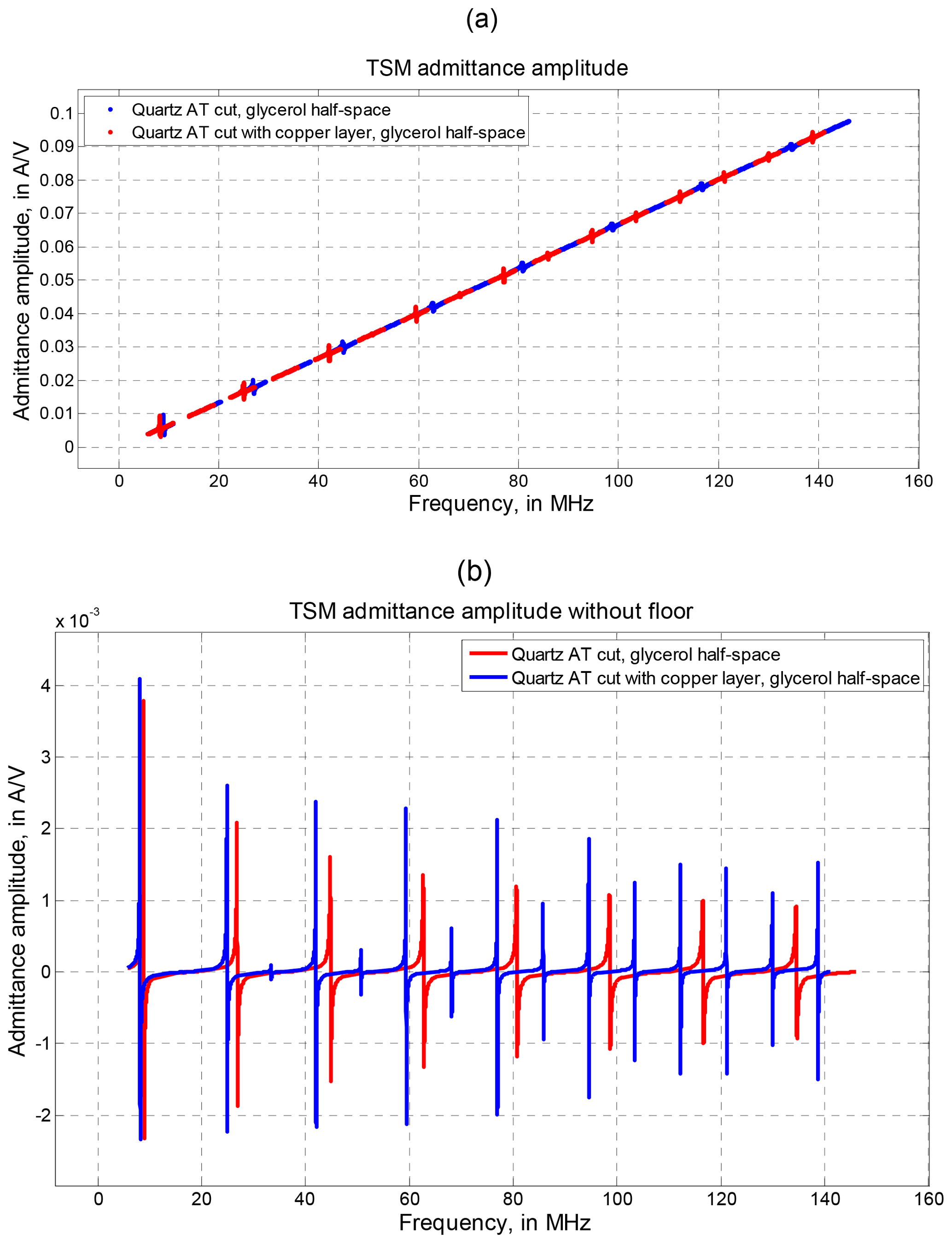
Figure 3 Calculated admittance amplitude as a function of frequency according to Eq. (32) for two cases of TSM material configurations: (1) AT-cut quartz plate with a liquid half-space of glycerol and (2) the same system as in (1), but with an additional copper layer below glycerol. The frequency range is extended over 16 resonances and anti-resonances; (a) with and (b) without floor signal.

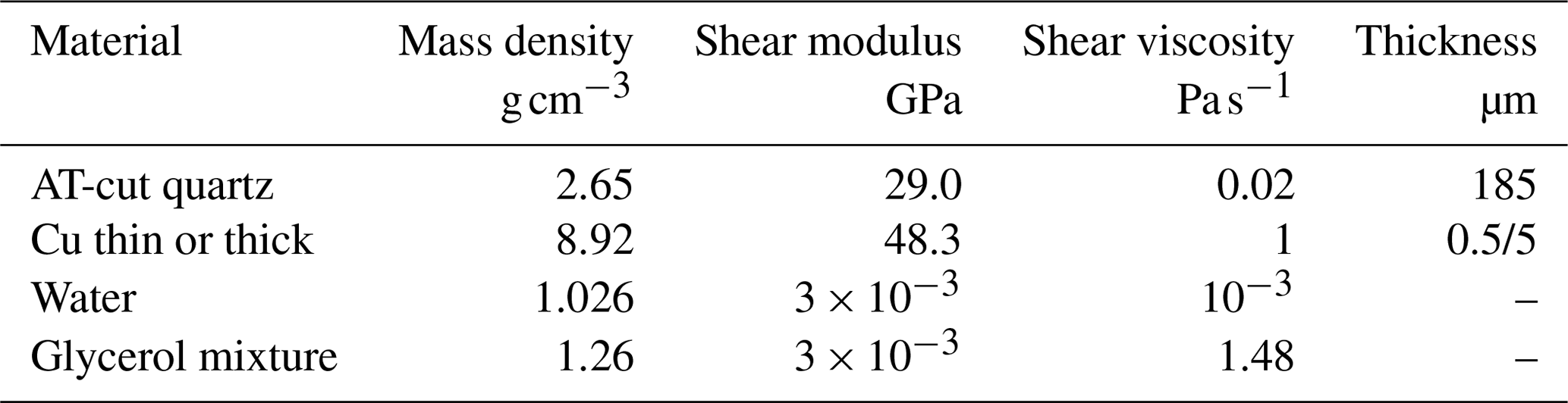
The remaining data applied for shear BAWs in AT-cut quartz are the piezoelectric stress constant 0.0958 A s m⁻² and relative permittivity of 4.533. The shear viscosity of 0.02 Pa s originates from a quality factor of 25 000 at 10 MHz.

In contrast to Fig. 3a, many more distinctive curves are obtained when subtracting the linearly frequency-dependent floor as seen in Fig. 3b. Such a procedure is simply realized and usually done in experiments, especially when keeping in mind that the floor originated from the capacitance C in Eqs. (28) and (32).

Figure 3b exhibits 16 resonance maxima of admittance amplitude accompanied by minima of anti-resonant frequencies positioned tightly above. The red curves (without any layer on the quartz plate) demonstrate rising resonances only at odd frequency harmonics, whereas when adding a 5 µm thick Cu layer, resonance peaks also arise at even harmonics (blue curves). Besides this, all resonance peaks are shifted to lower frequencies in that case.

Many attempts were made to find expressions for identifying material parameters directly from resonant frequency shifts. For example the well-known formulas of Sauerbrey (1959) and of Kanazawa and Gordon (1985) exist, but in each case with a limited range of validity. For example, according to Kanazawa the relative shift δf/f of TSM resonant frequency under the influence of a liquid with mass density ρ and shear viscosity η is approximately given by

$$\begin{array}{}\text{(34)}& {\displaystyle \frac{\mathit{\delta }f}{f}}\approx -{\displaystyle \frac{\sqrt{\mathit{\rho }\mathit{\omega }\mathit{\eta }/\mathrm{2}}}{\mathrm{2}{Z}_q}}.\end{array}$$

However, for large products (ρωη) the relative frequency shift δf∕f will indeed approach twice this value.

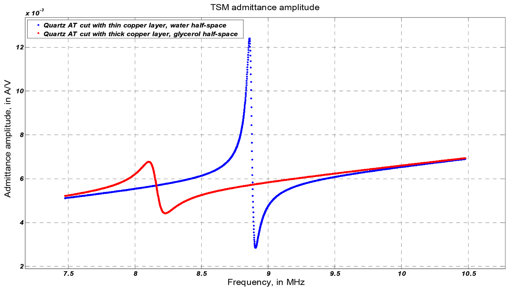
Figure 4 Admittance amplitude vs. frequency after removing the floor signal at fundamental resonance and anti-resonance. Considered material systems: quartz plate with thin Cu layer and water half-space (red curve) and quartz plate with thick Cu layer and glycerol mixture half-space (blue curve).

Two other examples of resonant behavior are depicted in Fig. 4. The curves are restricted to the fundamental resonance (1st harmonic). It is seen that there are not only reductions of resonant and anti-resonant frequencies by thickening the copper layer, but the widths of peak and anti-peaks are also increased when replacing natural water with a glycerol mixture in the upper half-space of the material system. The evaluation of the corresponding bandwidths by the parameter FWHM was introduced above.

Corresponding to the width of the resonance peak, the FWHM of anti-resonance is found using the curve of impedance instead of admittance amplitude. In sum we can extract M data from the measurements as follows:

$$\begin{array}{}\text{(35)}& M=\mathrm{4}{N}_{\mathrm{OT}}.\end{array}$$

These are the frequencies of resonance and anti-resonance (f_res and f_ares) and the differences of frequencies of the FWHMs (FWHM_res and FWHM_ares), with N_OT as the number of measured overtones.

3.2 Extractable parameters of material systems under study

Equation (32) enables us to come to significant conclusions of parameter extraction from TSM measurements. In connection with Eq. (33a, b, and c) the dependence on acoustic impedances Z and BAW propagation times τ is obvious. In more detail, all parts of the material system of Fig. 1 are involved:

$$\begin{array}{}\text{(36)}& Z^{-}\mathrm{\dots }{Z}^{\left(k\right)}{\mathit{\tau }}^{\left(k\right)}\mathrm{\dots }{Z}^{+}.\end{array}$$

The index k runs over all layers on both sides of the piezoelectric plate. We have to take into account that both quantities, Z and τ, can be valued as complex in consequence of viscous properties and thereby caused lossy behavior. As a result of this circumstance we are in the position to extract N material–geometric parameters with N⁺ and N⁻ as the bottom and top layer numbers, respectively, and N^half−space as the number of half-spaces:

$$\begin{array}{}\text{(37)}& N=\mathrm{4}{N}^{+}+\mathrm{4}{N}^{-}+\mathrm{2}{N}^{\mathrm{half}-\mathrm{space}}.\end{array}$$

Actual material–geometric parameters instead of Z and τ are mass densities ρ, elasticities c, and layer thicknesses d. They are related to each other according to Eqs. (20a), (20b), and (11a) applied for isotropic symmetry. In order to account for viscoelastic behavior we consider c to be complex:

$$\begin{array}{}\text{(38)}& c=G+j\mathit{\omega }\mathit{\eta },\end{array}$$

with G as the shear modulus and η as the shear viscosity. For simplicity, cases with behavior deviating from the widely used model Eq. (38) are not considered here. Instead of Eq. (36) the list of extractable material–geometric parameters is now as follows:

$$\begin{array}{}\text{(39)}& (\mathit{\rho }G{)}^{-},(\mathit{\rho }\mathit{\eta }{)}^{-}\mathrm{\dots }{\mathit{\rho }}^{\left(k\right)}{G}^{\left(k\right)},{\mathit{\eta }}^{\left(k\right)},d^{\left(k\right)}\mathrm{\dots }(\mathit{\rho }G{)}^{+},(\mathit{\rho }\mathit{\eta }{)}^{+}.\end{array}$$

Note that in the frame of our model of pure shear BAWs for the half-spaces, only products of ρ times G and of ρ times η can be determined. However, as a consequence of Eq. (32), a maximum of four parameters are detectable for each layer k.

3.3 Sensitivities of experimental data against extractable parameters

One decisive question in the procedure of multi-parameter sensing is the following: how many and which parameters can be extracted from the measurements, and under which conditions can they be extracted? It is obvious from the admittance curves of Fig. 3b that a considerable number of experimental data can be supplied to find out the related material and geometry parameters that produce such specific behavior. The essential point is the influence of the material parameters according to Eq. (39) on the list of measured frequencies, i.e., resonant and anti-resonant frequencies f_res and f_ares and the full widths at half maximum FWHM_res and FWHM_ares for a number of overtones N_OT including both odd and even harmonics.

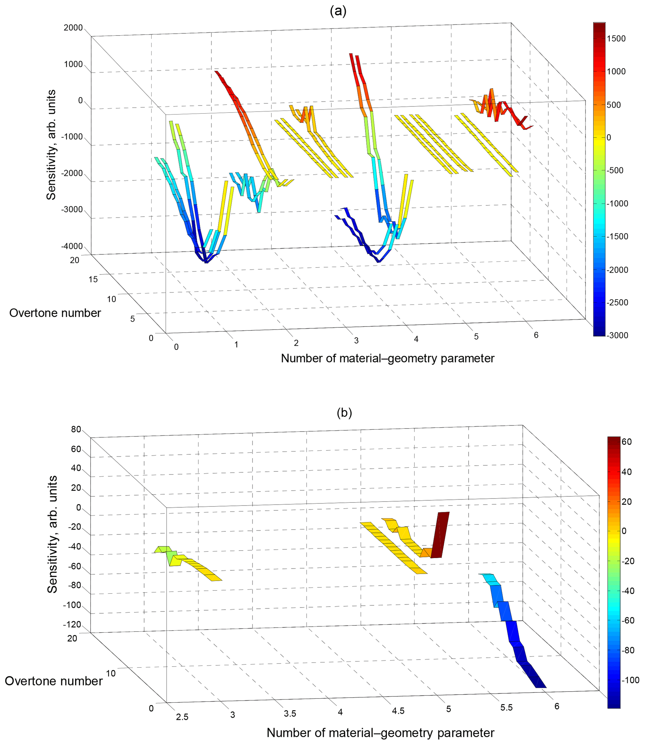
Figure 5 (a) Mapping of the elements of the Jacobian matrix J_mn defined in Eq. (40) with varying measurement index m from 1 to 56 and material parameter index n from 1 to 6. The overtone number runs from 1 to 16. The material system is an AT-cut quartz plate with a 5 µm thick Cu layer and a glycerol half-space. Order at each material–geometry parameter value: resonant–anti-resonant frequencies and resonant–anti-resonant FWHMs. (b) Mapping with enlarged sensitivity range around zero, at material parameter 3 (Cu viscosity) and 6 (glycerol viscosity × mass density) for the resonant frequencies and at material parameter 5 (glycerol shear modulus × mass density) for both resonant frequencies (left) and FWHMs (right).

Table 1 The used data of studied exemplary material systems.

The number of involved quantities produces some complexity in the problem. Forming the first derivatives of experimental data with respect to the searched parameters is a preferential method to elucidate the situation. Again, Eq. (32) is hereby appropriate for performing such numerical analysis and facilitates the approach. The aforesaid first derivatives represent the sensitivities of experimental data against extractable parameters. We start with values for the material–geometry parameters which are assumed to be reasonable, keeping in mind that for the possibility of parameter extraction at the end of the procedure, the use of sensitivities for that has to be considered in connection with their certainty or uncertainty. This means that it is advantageous to form a Jacobian matrix J_mn with the elements

$$\begin{array}{}\text{(40)}& {\mathbf{J}}_{mn}={\displaystyle \frac{\partial f_m}{\partial p_n}}{\displaystyle \frac{p_n}{\mathrm{\Delta }{f}_m}}.\end{array}$$

In this formula f_m denotes a measurement result such as resonant and anti-resonant frequency or the FWHM frequency difference with number m and p_n, a searched material–geometry value of parameter number n. The derivative $\partial f_m/\partial p_n$ is normalized here to the ratio of frequency uncertainty Δf_m and material parameter p_n. Under these conditions the elements of the matrix J_mn are dimensionless and incorporate a weighting factor for the preference of more accurate measurements. The uncertainties Δf_m depend on the specific conditions of the experiment. In our example we assumed amplitude uncertainties at resonant and anti-resonant frequencies of 10⁻⁵ and uncertainties of 10⁻² for the determination of the FWHM level.

Examples for sensitivities as functions of m and n are shown in Fig. 5a and b. The assignment of material–geometry parameters to the used numbers n is described in Table 2. The employed data of the studied material system are specified in Table 1.

Table 2 Numbering n of material–geometry parameters.

The structures depicted in Fig. 5 exhibit some features which can be employed for further refinement of multi-parameter search. The dependences of sensitivities J_mn on the overtone number seem to be very similar for resonance and anti-resonance behavior at a given parameter, i.e., a constraint on the resonance case seems satisfactory. It can be seen in Fig. 5 that in the analyzed material system (AT-cut quartz plate with a 5 µm thick Cu layer and a glycerol half-space), the highest sensitivities are achieved for the Cu mass density and thickness (parameter number 1 and 4).

Figure 6 Example of the environment of SSQ_min of the special case of AT-cut quartz TSM resonator with a 5 µm thick Cu layer that is in contact with glycerol. The varied material parameters are mass density (p₁) and shear modulus (p₂) of the Cu layer. The incorporated measurements comprise all resonant and anti-resonant frequencies and FWHMs until the 16th overtone (except 2nd and 4th).

Measurements at higher overtones seem more beneficial for the extraction of these parameters. Viscosities (parameter 3 for Cu and 6 for glycerol) are extractable from measured FWHM data, preferentially at high overtones. The sensitivities of resonant and anti-resonant frequencies vs. n=3 (Cu viscosity), 5 (glycerol shear modulus × mass density), and 6 (glycerol shear modulus × viscosity) and of FWHM vs. n=5 (glycerol shear modulus × mass density) seem to be too small for examination. Nevertheless, as can be seen from Fig. 5b, most of these results are also still worth evaluating. In the case of glycerol viscosity the FWHM curve is depicted vs. overtone number, and in the other three cases only the resonant frequency behavior is depicted.

4 Optimization of multi-parameter sensing approach

4.1 Evaluation of fitting procedure

The extraction of material–geometry parameters from TSM measurements requires a fitting procedure between theoretically and experimentally determined frequencies. A precedent examination of achievable results is important for avoiding unsuccessful calculation efforts originating from inappropriate selection of experimental results caused by marginal sensitivities. The outcome of such a study enables one to develop the strategy of fitting or, in other words, to optimize the multi-parameter sensing approach.

For that purpose the environment of the minimum of the sum of squared relative differences (SSQ) between theoretical and experimental values $f_m^{\mathrm{th}}$ and $f_m^{\exp }$, respectively, will be considered more in detail now. These differences are weighted by the inverse of uncertainties Δf_m, just as was done at the definition of matrix J_mn. The quantity SSQ has the form

$$\begin{array}{}\text{(41)}& \text{SSQ}=\sum _{m=\mathrm{1}}^M{\left({\displaystyle \frac{f_m^{\mathrm{th}}\left(p_n\right)-f_m^{\exp }}{\mathrm{\Delta }{f}_m}}\right)}^{\mathrm{2}},\end{array}$$

a sum over all M experiments, and varies due to changing parameters p_n. The fitting procedure will be performed until SSQ reaches a “very deep” minimum SSQ_min, preferably the so-called global minimum. At this location in the (N+1)-dimensional space all first-order derivatives of SSQ with respect to parameter p_n vanish. For the environment of this minimum we assume a quadratic dependence of SSQ on small relative changes in material–geometry parameters δp_n∕p_n and can write the following in matrix notation:

$$\begin{array}{}\text{(42)}& \text{SSQ}={\text{SSQ}}_{\min }+{\left(\mathit{\delta }p/p\right)}^{\mathbf{T}}\mathbf{H}\left(\mathit{\delta }p/p\right),\mathbf{H}={\mathbf{J}}^{\mathbf{T}}\mathbf{J}.\end{array}$$

J is the Jacobian matrix with the elements J_mn introduced in Eq. (40), p stands for p_n, and δp∕p stands for δp_n∕p_n. T denotes the transposed expression. The environment of SSQ_min is determined by the symmetric matrix H, with rows and columns given by the number N of searched parameters p_n. At a given SSQ above SSQ_min the variations δp_n∕p_n will form an ellipsoid in the N-dimensional space of material parameters.

An illustration of the situation is given in Fig. 6. The considered sample is an AT-cut quartz TSM resonator, with a thickness 185 µm, coated by a 5 µm thick Cu layer and a glycerol half-space on top. As can be seen, the variation of SSQ produces ellipses in the two-dimensional space of the two material parameter variations δp₁ (change in mass density) and δp₂ (change in shear modulus of Cu layer). If H is a diagonal matrix, then the directions of the δp_n axes coincide with the directions of the half-axes of ellipses. In this case Eq. (42) is a sum of single squared relative material parameter changes ${\left(\mathit{\delta }{p}_n/p_n\right)}^{\mathrm{2}}$, and all material parameters contribute independently of each other to the SSQ. Inversely, at a given SSQ each single parameter deviation δp_n∕p_n can be derived separately.

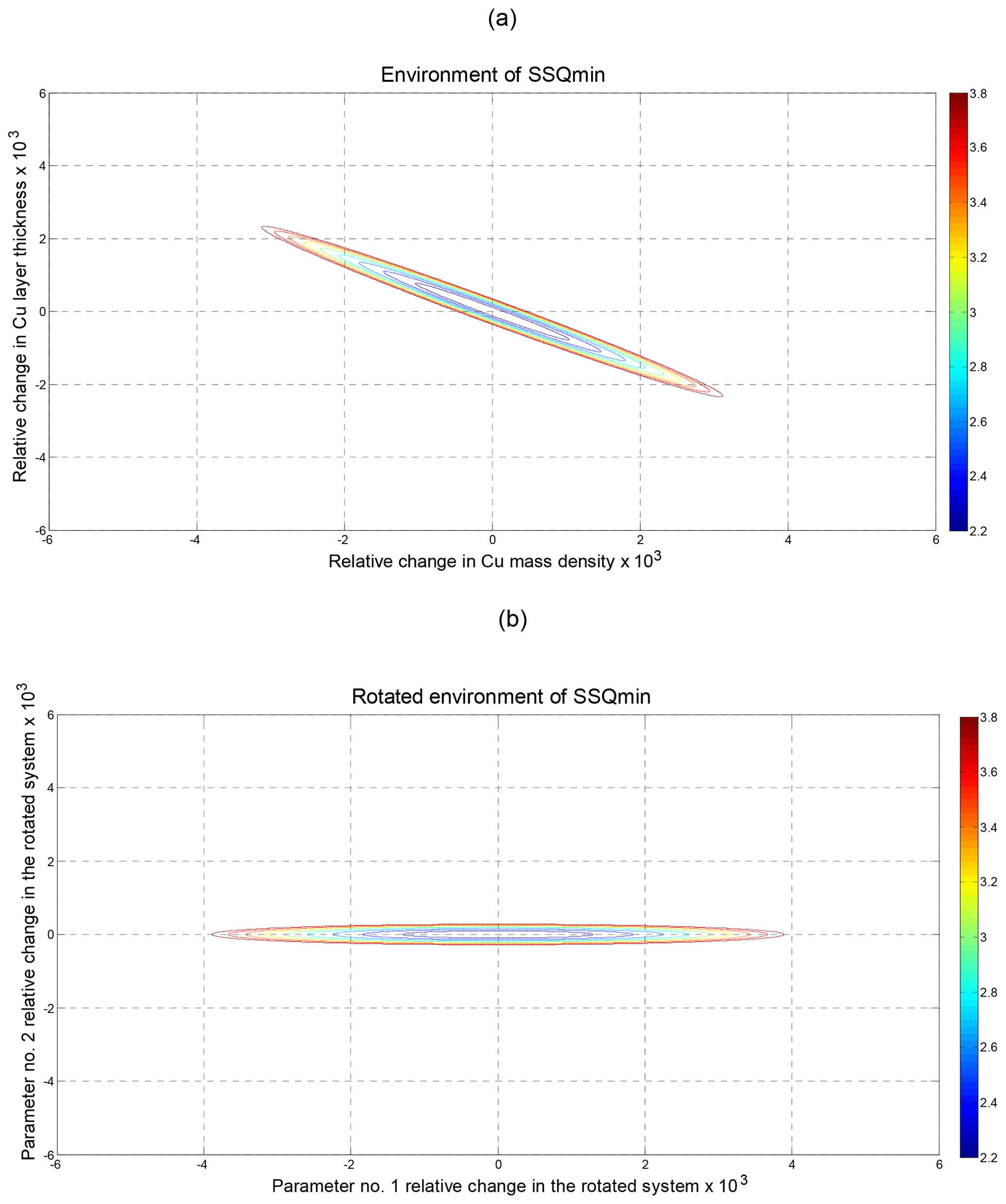
Figure 7 (a) Example of ellipses in the plane of two material–geometry parameters created by constant SSQ>SSQ_min. Material system: AT-cut quartz TSM resonator with a 5 µm thick Cu layer that is in contact with glycerol. The varied material parameters are mass density and thickness of the Cu layer. The incorporated measurements are the resonant and anti-resonant frequencies of the 3th and 5th overtones. (b) Ellipses aligned with the material–geometry parameter axes after the orthogonal transformation of the parameter space.

However, in the very most cases H is not a diagonal matrix, and a direct derivation of material parameter deviations δp_n from a given SSQ is not possible. An extreme case for two parameters is depicted in Fig. 7a. The half-axes of ellipses deviate strongly here from the axes of δp₁ and δp₂. As a consequence, the deviation δp₁ at a given δp₂=0 and also δp₂ at δp₁=0 are inappropriately small in view of the length of the ellipse. Therefore, the correct evaluation of parameter deviations δp_n requires an orthogonal transformation of the space of N material parameters for obtaining a diagonal matrix H^′ instead of H:

$$\begin{array}{}\text{(43)}& {\mathbf{H}}^{\prime }={\mathbf{Q}}^{\mathrm{T}}\mathbf{HQ},\end{array}$$

with Q as a matrix formed by the N eigenvectors yielded by the eigenvalue procedure for the diagonalization of H. This leads to the situation of Fig. 7b.

Figure 8 Flow chart of the approach to multi-parameter sensing of layers and half-spaces that are in contact with a TSM resonator.

4.2 Determination of uncertainties of extracted parameters

A key question for the experimental strategy of identifying material–geometry parameters is how to achieve high accuracy with a low number of experiments. Answers can be found on the basis of supposed appropriate initial values for the searched parameters and by analyzing the environment of the SSQ.

A self-evident value for a given uncertainty $\mathrm{\Delta }\mathrm{SSQ}=\mathrm{SSQ}-{\mathrm{SSQ}}_{\min }$ is the total number M of measurements. This is plausible when considering Eq. (41) and making use of the simple approach where in the middle, for each measurement m, the assumed uncertainty Δf_m equals the difference $f_m^{\mathrm{th}}-f_m^{\exp }$. In that case all the contributions to ΔSSQ are equal to 1, and the summation over m yields the value M. At a given uncertainty ΔSSQ=M the uncertainties of relative material parameters $(\mathrm{\Delta }{p}_n/p_n{)}^{\prime }$ in the transformed material parameter space can now be written by taking into account the N-fold partition of ΔSSQ, with ${\mathbf{H}}_{nn}^{\prime }$ as the nth diagonal element of matrix H^′:

$$\begin{array}{}\text{(44)}& {\left(\mathrm{\Delta }{p}_n/p_n\right)}^{\prime \mathrm{2}}={\displaystyle \frac{M/N}{{\mathbf{H}}_{nn}^{\prime }}}.\end{array}$$

The next step is the back transformation to the original space of material parameters. In order to find the squared uncertainties Δp_n∕p_n we have to sum up the retransformed squared uncertainties:

$$\begin{array}{}\text{(45)}& {\left(\mathrm{\Delta }{p}_n/p_n\right)}^{\mathrm{2}}=\sum _{m=\mathrm{1}}^M{\left({\mathbf{Q}}_{nm}{\left(\mathrm{\Delta }{p}_m/p_m\right)}^{\prime }\right)}^{\mathrm{2}}.\end{array}$$

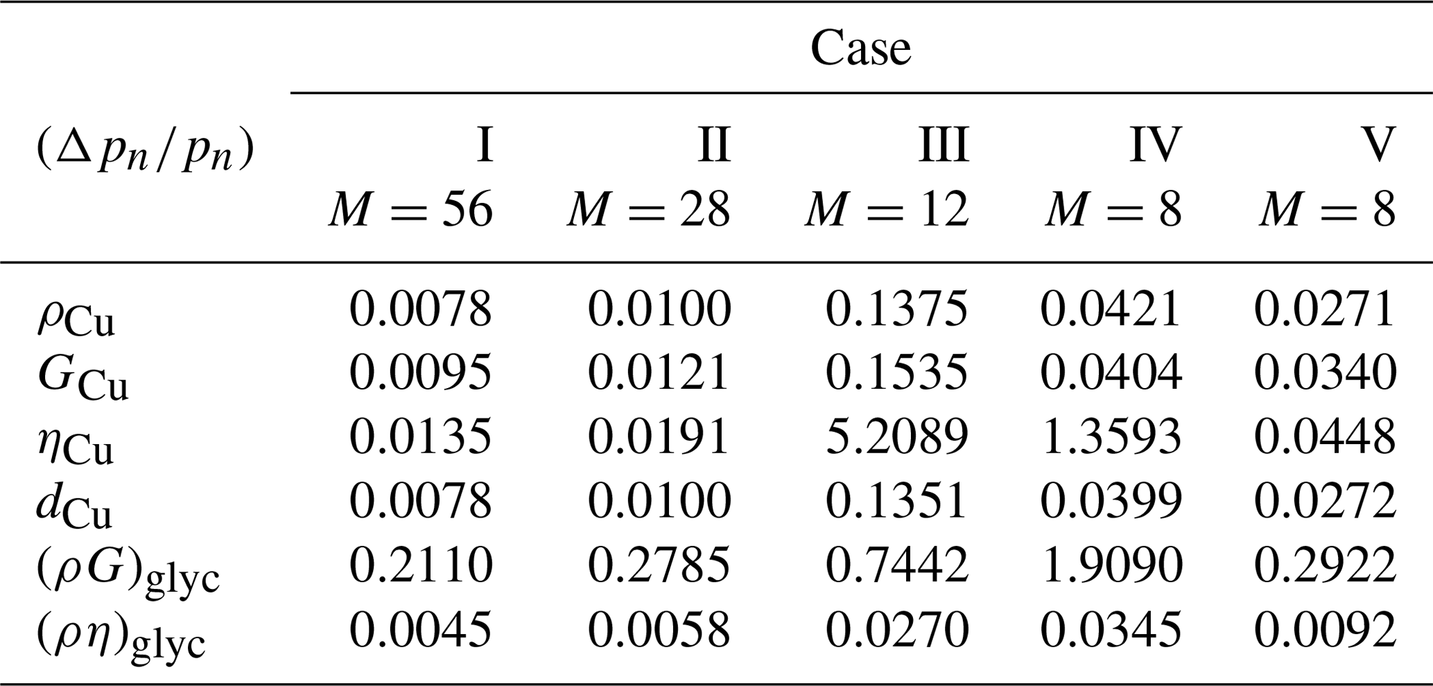
Table 3 provides insight into a series of different combinations of experiments in order to obtain the full set of six material–geometry parameters of the system, already considered in Sect. 3.3 with respect to the achieved uncertainties. The columns I to V depict different cases.

• Case I corresponds to the full set of resonant and anti-resonant frequencies and FWHMs of 1st, 3rd, and 5th–16th harmonics.

• Case II is, compared to I, restricted to the resonances.

• Case III is the combination of 1st, 3rd, and 5th overtones.

• Case IV is the full set of 5th and 6th overtones.

• Case V is yielded by a combination of anti-resonant frequency of the 1st harmonic, resonant frequency of the 16th overtone, resonant FWHMs of the 1st and of the 16th overtone, and anti-resonant FWHMs of the 3rd, 5th, 6th, and 8th overtones.

The corresponding numbers M of measurements are indicated. From Table 3, the following can be seen.

• There is only small worsening when restricting the full set of measurements to resonant frequencies and resonant FWHMs (case II compared to case I).

• Cases III and IV suggest that a strong reduction of the measurement number can produce inadmissibly high uncertainties.

• Case V, unlike III and IV, exhibits acceptable small uncertainties in the face of reduction of experimental efforts compared to I by a factor of 7.

Table 3 Uncertainties of material–geometry parameters of the material system described in Sect. 3.3. The columns are related to five different combinations of measurements.

5 Conclusions

Based on an extra derived analytic expression (Eq. 32) for the frequency dependence of electrical admittance, the suitability of a TSM resonator for multi-parameter sensing of layers and half-spaces that are in contact with the resonator plate on both sides has been analyzed. Resonant and anti-resonant frequencies as well as related bandwidths (FWHMs) were considered to be dependent on material–geometry parameters to calculate sensitivities of these experimental values against the searched parameters. This Jacobian matrix was used to evaluate the environment of the minimum of fitting procedure between experimental and theoretical values as a function of all material–geometry parameter variations, with the aim of obtaining their uncertainties after extraction from the experimental results. The separation of uncertainties of searched parameters requires a back-and-forth orthogonal transformation in the parameter space for the diagonalization of the squared Jacobian matrix.

Figure 8 summarizes the procedure for realizing multi-parameter sensing of layers and half-spaces that are in contact with a TSM resonator as it was carried out in this study, using an analytic expression for the electrical admittance.

It was shown for the special case of a TSM resonator of AT-cut quartz coated by a 5 µm thick copper layer and a glycerol half-space on top that six parameters of layers and half-spaces can be determined. At the reduction of the number of used experimental data from 56 to 8, a special combination of measurements with only a small increase in parameter uncertainties was found. An optimal selection of experimental data for uncertainty minimization exhibits some plausible relationships, for example the preference of FWHM instead of resonant frequency measurements for the determination of viscosities.

The demonstrated procedure is suitable for developing an experimental strategy for multi-parameter sensing involving both the minimization of parameter uncertainties as well as of experimental effort.