the Creative Commons Attribution 4.0 License.
the Creative Commons Attribution 4.0 License.
 | 31 Jul 2020
Measurement uncertainty analysis of field-programmable gate-array-based, real-time signal processing for ultrasound flow imaging
Richard Nauber
Lars Büttner
Jürgen Czarske
Research in magnetohydrodynamics (MHD) aims to understand the complex interactions of electrically conductive fluids and magnetic fields. A promising approach for investigating complex instationary flow phenomena are lab-scale experiments with low-melting alloys. They require a noninvasive flow instrumentation for opaque liquids with a high spatiotemporal resolution, a low velocity uncertainty and a long measurement duration. Ultrasound Doppler velocimetry can achieve multiplane, multicomponential flow imaging with multiple linear ultrasound arrays. However the average raw data output amounts to 1.2 GBs−1 at a frame rate of 33 Hz in a typical configuration for 200 transducers. This usually prevents long-duration measurements when offline signal processing is used.
In this paper, we propose an online signal-processing chain for pulsed-wave Doppler velocimetry that is tailored to the specific requirements of flow imaging for lab-scale experiments. The trade-off between measurement uncertainty and computational complexity is evaluated for different algorithmic variants in relation to the Cramér–Rao bound. By utilizing selected approximations and parameter choices, a prepossessing could be efficiently implemented on a field-programmable gate array (FPGA), enabling a typical reduction of the data bandwidth of 6.5:1 and online flow visualization. We validated the performance of the signal processing on a test rig, yielding a velocity standard deviation that is a factor of 3 above the theoretical limit despite a low computational complexity.
Potential applications for this signal processing include multihour flow measurements during a crystal-growth process and closed-loop velocity feedback for model experiments.
- Article
(1085 KB) - Full-text XML
- BibTeX
- EndNote


Many important industrial processes, such as continuous steel casting and photovoltaic wafer production, involve metal or semiconductor melt flows. The quality of the product and the energy efficiency of the process strongly depends on the flow behavior of the liquid (Müller and Friedrich, 2010; Gardin et al., 1995; Yasuda et al., 2007). A noncontact way of influencing the flow of electrically conductive melts is the application of magnetic fields that introduce Lorentz forces to the fluid. Investigating the interaction of a magnetic field with the flow pattern and optimizing the spatiotemporal structure of the magnetic field for different applications are subjects of ongoing research in magnetohydrodynamics (MHD). Besides numerical simulations, low-temperature, model-scale experiments are important tools for MHD investigations (Eckert et al., 2007b). They often require advanced flow instrumentation for visualizing complex and instationary flows in opaque liquids. A typical set of requirements for MHD research are as follows:
-
Noninvasiveness – the influence of the instrumentation to the flow should be negligible (Eckert et al., 2007a).
-
Flow imaging capability – the fluid's velocity should be visualized in multiple planes (2D) with two or three velocity components (2c or 3c) in order to adequately represent complex flow patterns.
-
Spatial resolution – the relevant flow structures have to be resolved, typically in the range of 10 mm (Timmel et al., 2011).
-
Temporal resolution – fluctuations (typically at 1 … 5 Hz) have to be resolved in order to capture instationary flows (Timmel et al., 2011).
-
Long measurement duration – flow phenomena on different timescales should be adequately captured; for instance, rapid spontaneous changes of the flow regime in a rotating flow (Galindo et al., 2017) or in multihour model experiments of the semiconductor crystallization process (Thieme et al., 2017).
-
Capability of near-wall measurements – in typical MHD experiments, the metal melt is contained in a vessel. The vicinity of the wall is especially important because the Lorentz force is often concentrated in this region. Contrary to, for instance, medical applications, the walls can be seen as completely stationary in most cases.
-
Online capability – conducting long-running MHD experiments requires the ability to examine the data during the duration of the measurement. Some model experiments in the semiconductor crystallization process even benefit from an active control of parameters, like magnetic field intensity and temperature gradient, based on the feedback from online velocity data to stabilize the flow (Thieme et al., 2017).
A measurement system for flow mapping of opaque liquids, namely the ultrasound array Doppler velocimeter (UADV; Nauber et al., 2013a, b), was presented in previous publications. It extends the pulsed-wave Doppler principle (Takeda, 1986; Baker, 1970) by employing multiple linear sensor arrays to achieve multiplane, two-componential flow imaging. The sensors are designed to achieve a lateral resolution of ≈3 mm in Galinstan (GaInSn). A combination of spatial- and time-division multiplexing allows one to parallelize the scanning process for a planar velocity map; hence increasing the temporal resolution compared to a strict sequential scan. However, online processing of the data for 200 transducer elements simultaneously on 32 channels at a temporal resolution typically of 33 Hz overburdens PC-based hardware with 1.2 GBs−1. Therefore, only discontinuous offline measurements could be performed with a limited duration of a few seconds. This severely impedes the usability of the UADV in the context of MHD experiments and restricts the investigations into stationary or periodic flows.
Although several investigations on the measurement uncertainty of Doppler velocity estimation methods for laser-based instrumentation (Fischer et al., 2010), for flow-rate measurements in a pipe (Furuichi, 2013), and for blood-flow measurements in the human body (Lovstakken et al., 2007) have been performed, no comprehensive measurement uncertainty budget in the context of instrumenting an MHD experiment has been presented to the knowledge of the authors.
This paper provides a signal-processing chain that is tailored to the specific requirements of MHD model experiments and shows a real-time implementation using a field-programmable gate array (FPGA). It enables the UADV system to perform long-duration measurements with high frame rates and online flow visualization. Furthermore, we evaluate the measurement uncertainty of the whole UADV system in the context of MHD experiments and present an uncertainty budget according to the methodology proposed by the “Guide to the expression of uncertainty in measurement” (GUM; JCGM, 2008) for a typical configuration.
2.1 Measurement principle
In pulsed-wave ultrasound Doppler velocimetry (PW–UDV), short bursts are emitted periodically with a pulse repetition frequency fPR (Baker, 1970). The emission times span the so-called slow-time axis ts, with nb=0…NEPP being the bursts number. The emitted bursts usually consist of Nperiods periods of a sinusoidal wave, with the frequency f0. As the bursts travel through the fluid, scattering particles reflect a fraction of the signal back to the ultrasound transceiver. The received echo signal z(tf, ts) is acquired, starting from the emission time along the fast-time axis tf. Figure 1 depicts an example of the echo signal for a single moving scattering particle.
The movement of a scattering particle leads to a phase shift of the echo signal between multiple burst emissions (Kasai et al., 1985). The mean phase shift per time unit, expressed as mean frequency fd, is related to the velocity v for a given speed of sound c by the following:
with ftx denoting the mean frequency of the received signal burst and c≫v. The mean phase shift per time unit fd can be interpreted as a Doppler frequency shift fd (Kasai et al., 1985); hence the name Doppler velocimetry.
The time since the burst emission tf corresponds to the distance d between the scattering particle and the transducer according to the following equation:
This allows a spatially resolved flow measurement along the axis of the transducer, given that the scattering particles follow the motion of the fluid with negligible slip. The axial resolution can be estimated with the following (Jensen, 1996):
The lateral resolution Δx is given by the width of the ultrasound beam, which is a result of the transducer geometry, the frequency f0, and the speed of sound c in the fluid. The temporal resolution Δt of the velocity measurement is determined through the following:
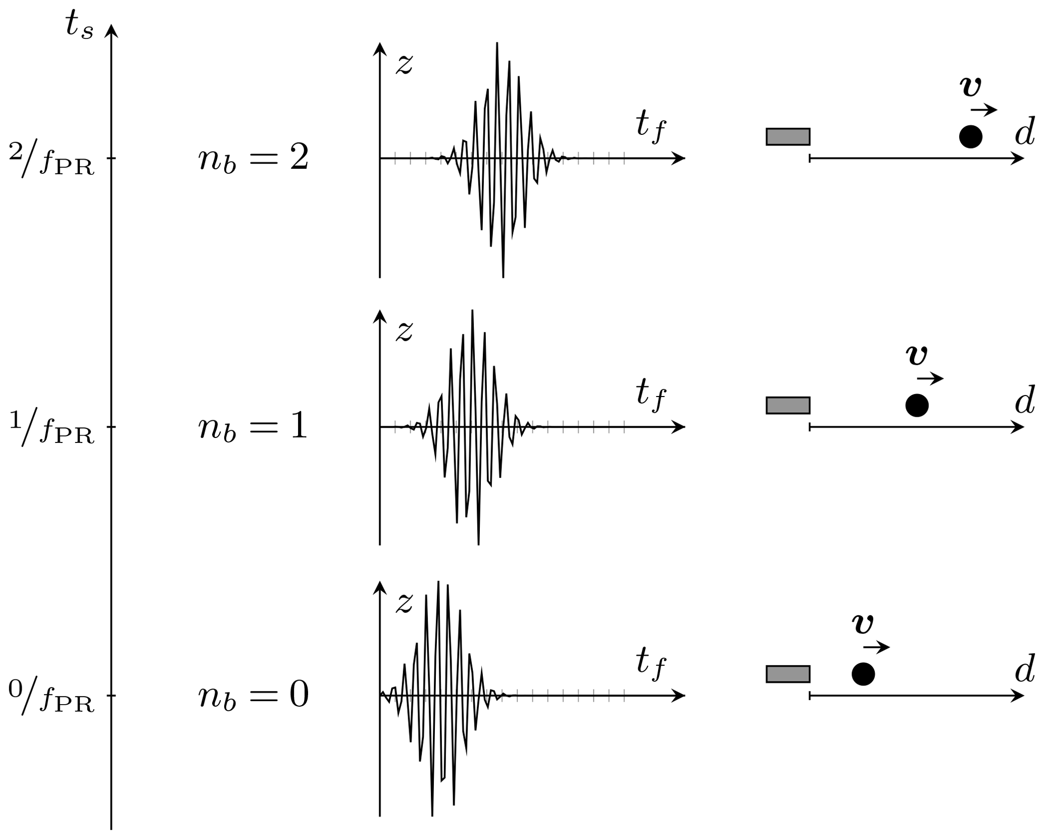
Figure 1PW–Doppler principle: multiple bursts are emitted at , with a repetition rate fPR. This constitutes the slow-time axis ts. After emission, the received echo signals are sampled with a frequency fs along the fast-time axis tf. The echo signal phase shift corresponds with the velocity of the scattering particles in the fluid. An example of a single particle moving away from the transducer is given.
2.2 Ultrasound array Doppler velocimeter
The ultrasound array Doppler velocimeter (UADV) is a modular research platform developed at the Laboratory of Measurement and Sensor System Technique (MST) for flow imaging in opaque liquids with PW–UDV. It is flexible and especially well suited for instrumenting a wide range of experiments in the field of MHD. The hardware of the UADV consists of individually configurable modules driving 25 ultrasound transducers each. It can be scaled to support up to 200 transducers in various configurations; for instance, in four linear arrays which can be individually parameterized regarding ultrasound frequency, pulse shape and length, and pulse-repetition frequency (Nauber et al., 2016; Büttner et al., 2013).
A module of the UADV consists of an arbitrary function generator and a power amplifier for generating parameterizable burst signals which are routed through a programmable switching matrix and a transmit/receive switch to the transducers. The received echo signals are amplified with a parametric gain and routed to the digitization unit. A single microcontroller-driven control unit provides the overall synchronization and the communication with the host PC. Using a combined spatial- and time-division multiplexing scheme, an ultrasound transducer array can scan a measurement plane at higher rates than a strict sequential scan. The UADV supports four independent digitization channels per module. The detailed description of the measurement system is given in Nauber et al. (2016).
3.1 Overview
The signal processing for PW–UDV can generally be classified into wideband and narrowband techniques; a comprehensive comparison is given by Torp et al. (1993). While parts of the signal processing in the radio frequency (RF) band can be realized in analog circuitry (Shung, 2015), fully digital implementations have found widespread use in the last decades because of the availability of fast digitizers and the increased flexibility and robustness of such approaches. To simultaneously handle a high number (e.g., 32) of channels through a fully digital signal-processing chain, very large data bandwidths have to be processed. This can be achieved by utilizing the parallel-processing capability of a field-programmable gate array (FPGA). Especially narrowband algorithms are very suitable for FPGA-based implementations, due to their low computational complexity (Alam and Parker, 2003; Loupas et al., 1995a). Therefore, this paper focuses on investigating the most common narrowband method, the velocity estimator by Kasai et al. (1985) and the extensions proposed by Loupas et al. (1995b).
A typical narrowband signal-processing chain is shown in Fig. 2. In this fully digital realization, the slow time ts is sampled for each burst nb at and the fast time tf is sampled with a frequency fs as follows:
The signals are then bandpass filtered to reduce noise contributions outside of the bandwidth of the transmitted ultrasound signal. A quadrature demodulation is performed, consisting of a Hilbert transform and a subsequent down sampling. Static echoes are removed through a clutter reduction filter (CRF) and the velocities are estimated by an autocorrelation.
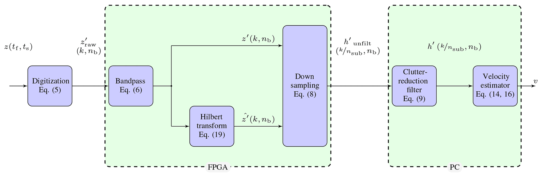
Figure 2Signal flow for a typical implementation of the Kasai algorithm: raw echo signals are bandpass filtered, quadrature demodulated and down sampled. The subsequent operations are performed on the complex demodulated signals, namely clutter-reduction filtering and velocity estimation.
3.2 Quadrature demodulation
In order to meet the assumptions of the narrowband signal processing and to reduce the influence of noise, a bandpass filtering is performed as follows:
with the filter coefficients ci. In order to maximize the SNR for signals with additive white Gaussian noise, a matched filter is used (Turin, 1960) as follows:
with the transmitted signal stx with Ntx samples.
The result of the quadrature demodulation is a complex signal in the baseband, which can be sampled at a lower rate (reduction by a factor of nsub) than the raw signal, as follows:
with and the Hilbert transform signal (with 90 ∘ phase shift with respect to z′).
3.3 Clutter-reduction filtering
A common problem of ultrasound Doppler flow measurements is distinguishing between static echoes originating from the walls (the so-called clutter) and echoes originating from scattering particles. Multiple reflections from the transmitted burst inside the wall superimpose the signal from scatter particles in the vicinity of the wall. For this problem, a multitude of signal-processing methods were proposed, most of them based on digital filters (finite impulse response (FIR) or infinite impulse response (IIR) filters) with various initialization techniques (Lee et al., 2009). With these methods, the clutter is distinguished from the particle echoes by a velocity close to zero, respectively, by a Doppler frequency shift close to zero. Because filtering will influence the spectrum of the signal, a bias may be introduced to the subsequent velocity estimation, depending on the frequency cutoff. For typical MHD experimental setups, the wall can be assumed to be completely stationary (in contrast to, e.g., medical applications where clutter is often constituted by slowly moving tissue; cf. Jensen, 1996); therefore, a steep cutoff at a frequency of zero is desirable. The simplest and computationally most efficient approach is to filter the constant component of the demodulated IQ signal by subtracting its mean value, which is the equivalent of applying a very narrow-band, high-pass filter (Thomas and Hall, 1994; Jensen, 1996; Torp, 1997; Bjaerum et al., 2002) as follows:
As the filter is noncausal, all NEPP samples have to be acquired before the result can be computed.
3.4 One-dimensional autocorrelation algorithm
A widely used approach for velocity estimation is the autocorrelation method proposed by Kasai et al. (1985), which operates solely in the domain of IQ-demodulated echo signals and therefore can be implemented very efficiently (Alam and Parker, 2003). It uses the properties of the signals' discrete autocorrelation function as follows:
where its values at a lag of 1 relate to the center of mass of the signal's power density spectrum through the Wiener–Khinchin theorem. As shown by Kasai et al. (1985) and Jensen (1996), the mean Doppler shift fd can be approximated through evaluating the autocorrelation function at a lag of Δnb=1 slow-time samples as follows:
This autocorrelation computation can be expressed solely by repeatedly multiplying accumulate operations and therefore can be implemented very efficiently. Kasai's method approximates the center frequency fd of the received signal with the frequency of the emitted signal as follows:
Being based on a phase estimation, the Kasai algorithm is inherently limited in the maximum measurable velocity. Given the 2π-phase ambiguity in Eq. (11), the measurable velocity range resulting from Eq. (1) is (Jensen, 1996) as follows:
3.5 Two-dimensional autocorrelation algorithm
An extension of Kasai's autocorrelation method is proposed by Loupas et al. to improve its performance in the following two regards (Loupas et al., 1995b):
-
The assumption of an unchanged center frequency of an ultrasound burst throughout emission, propagation inside the fluid and reception is discarded. This allows one to account for the effect of frequency-dependent attenuation, which is present in most relevant fluids. By explicitly estimating the center frequency of the received signal, a systematic velocity error stemming from the relationship in Eq. (1) is avoided.
-
An information loss occurs if only a narrow-band part of a broadband echo signal is processed. Hence a better estimation of the velocity is achieved by including a larger part of the signal spectrum.
Both aspects are addressed by increasing the dimensionality of Kasai's autocorrelation; instead of just correlating along the slow-time axis, a 2D autocorrelation along the slow- and fast-time axis is performed. An autocorrelation with a lag of one fast-time sample yields the estimate of the center frequency as follows:
Furthermore, the estimation of the frequencies ftx and fd can be performed using M samples per gate, as follows:
The extension of the Kasai autocorrelation algorithm potentially improves the estimation performance while still preserving a low computational complexity.
In order to provide online capability, the signal processing depicted in Fig. 2 has been realized on an FPGA (NI PXIe-7965R; National Instruments, Austin, Texas, USA). The FPGA communicates with a host PC through a peripheral component interconnect express (PCIe) bus and has the ability to stream data through direct memory access into the main memory of the PC.
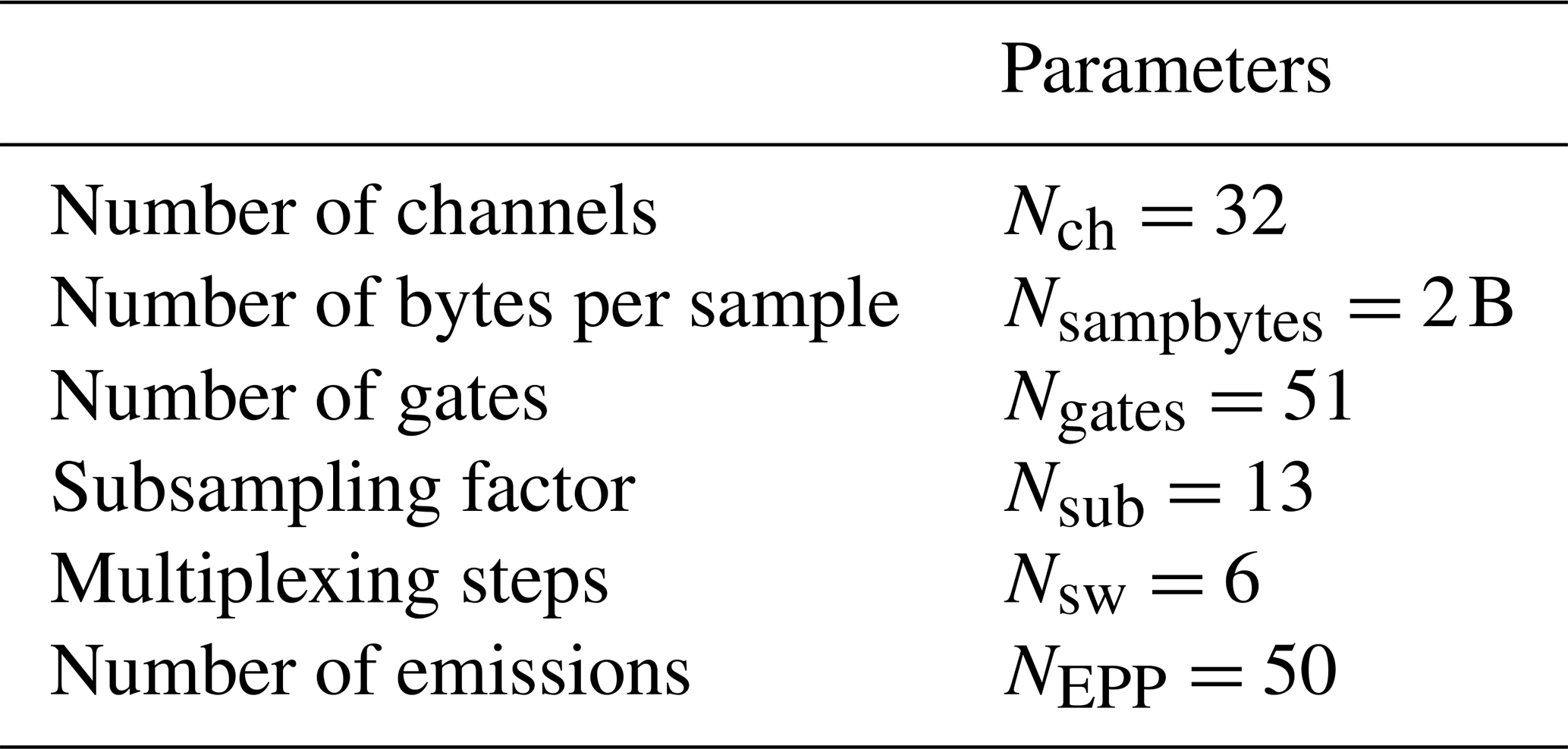
The amplified echo signals () are digitized through an A/D converter module (NI-5752; National Instruments, Austin, Texas, USA) for nch=32 channels at an externally provided sampling rate with a quantization of 12 bit. The raw data rate rADC at this stage is as follows:
Data are processed as signed 16 bit integer (nsampbytes=2 B) and, for a typical configuration as listed in Table 1, the data rate amounts to 1.2 GBs−1.
This data bandwidth is hardly suitable for continuous streaming to a storage device over a long duration (>1 h) with common PC hardware. Therefore, raw data are only briefly retrieved for debugging purposes or for low frame-rate measurements and are otherwise not transferred to the host.
The signal-processing steps that perform an IQ demodulation (bandpass filtering, Hilbert transform and down sampling) are significantly reduced in their computational complexity by fixing the ratio of the sampling frequency fs to the ultrasound center frequency f0 at . The matched filter can be realized for a sinusoidal transmit signal at ftx with Nperiods periods, assuming ftx≈frx with only trivial filter coefficients ci, as follows:
This allows one to implement the filtering without multiplication operations, only negations and additions are needed.
To provide a low computational complexity approximation of the Hilbert transform for a narrowband case, a fixed time delay can be employed (Kantz et al., 2012) as follows:
where . The signal processing up to this point contains just the summation, negation and storage primitives and therefore can be implemented on an FPGA with modest resources. The data rate rIQ at this stage for a typical configuration is given by the following:
Through the data reduction of 6.5:1, the data rate at this stage is for a typical configuration, as listed in Table 1. A continuous data streaming to a storage device can be sustained for a long duration at this rate.
5.1 Theoretical limit of measurement uncertainty
In order to characterize the performance of a signal-processing algorithm, it is not only helpful to have relative data compared to other algorithms but also to relate it to a fundamental limit of attainable precision. This absolute limit of uncertainty can be provided by means of the estimation theory using the Cramér–Rao bound (CRB; Radhakrishna Rao, 1945; Cramér, 1946). Given a suitable signal model, the CRB represents the lowest possible variance for estimating a parameter from the signal with an unbiased estimator. In the following, a simple signal model for a discrete time idealized ultrasound echo is described and a derivation of the CRB for velocity estimation is given.
A simple approximation of the ultrasound echo signal realizations consists of a sinusoidal signal superimposed with additive white Gaussian noise sparsely and periodically sampled in the fast- (k) and slow-time (nb) axis as follows:
and A being the amplitude of the scattering particles' echo, φ0 a constant phase, and Gaussian white noise, with a variance and zero mean.
The unknown quantities are as follows:
The CRB provides the lower boundary for the variance of an estimator according to the inequality, as follows:
with I(θ) being the Fisher information matrix, as follows:
Kay (1993) provided a formula for the case when the probability density function p(x, θ) of the signal model x, Eq. (22), is a Gaussian joint probability function as follows:
The differentiation of with respect to the unknown quantities is performed analytically, while the matrix inversion was performed numerically using MATLAB (The MathWorks, Inc., Natick, Massachusetts, USA). The resulting CRB for the velocity uncertainty as a function of the signal-to-noise ratio (SNR) is given in Fig. 4c–d. It has a slope of −20 dB/decade, which is consistent with the CRB of other Doppler-based signal-processing problems (Fischer et al., 2010; Chan et al., 2012; Demirli and Saniie, 2001).
5.2 UADV measurements on a reference experiment
For an experimental characterization of the measurement performance of the UADV system, a test rig based on the linear translation of a single scattering object is used (Fig. 3). It consists of a linear stage (41.121.102E; OWIS GmbH, Staufen, Germany) that is mounted over a glass tank with the dimensions of . It moves a scattering object (glass fiber with a spherical tip, and diameter of 0.6 mm, mounted in a hollow needle) with a constant velocity through water (; ). The ultrasound sensor array is mounted on the front wall of the tank and therefore insonates through an 8 mm glass wall and a water-based ultrasound couplant.
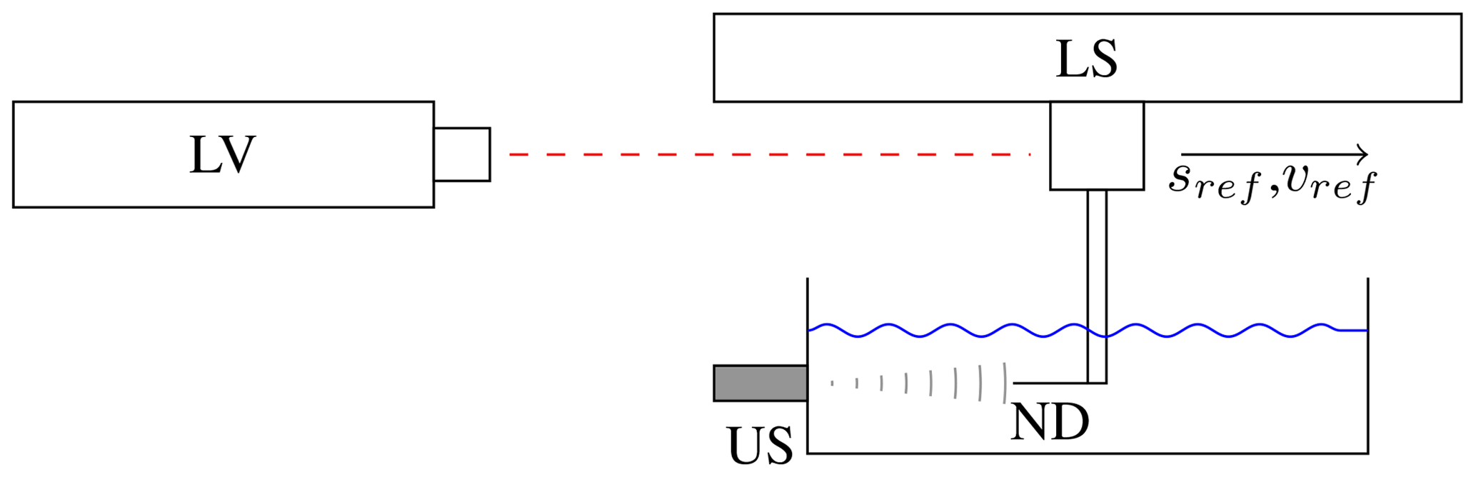
Figure 3A measurement setup in which the tip of a glass fiber is mounted on a needle (ND) is insonified by an ultrasound transducer (US) and moved by a linear translation stage (LS). A laser vibrometer (LV) measures its velocity (vref) and position (sref).
In order to trace back the measurement results of the UADV to the definitions of the respective units in the SI system, a simultaneous measurement of the relative position and velocity was done with a vibrometer (OFV-503; Polytech, Waldbronn, Germany; displacement decoder DD-900 and velocity decoder VD-09). A retroreflective tape (3M Scotchlite) was attached to the shaft of the scattering object's mount. For a velocity set point of 10 mms−1, a standard deviation of the velocity was determined for the linear stage–vibrometer combination (for the same averaging time as the UADV system).
Table 2Overview of the ultrasound parameters and the signal-processing algorithms.
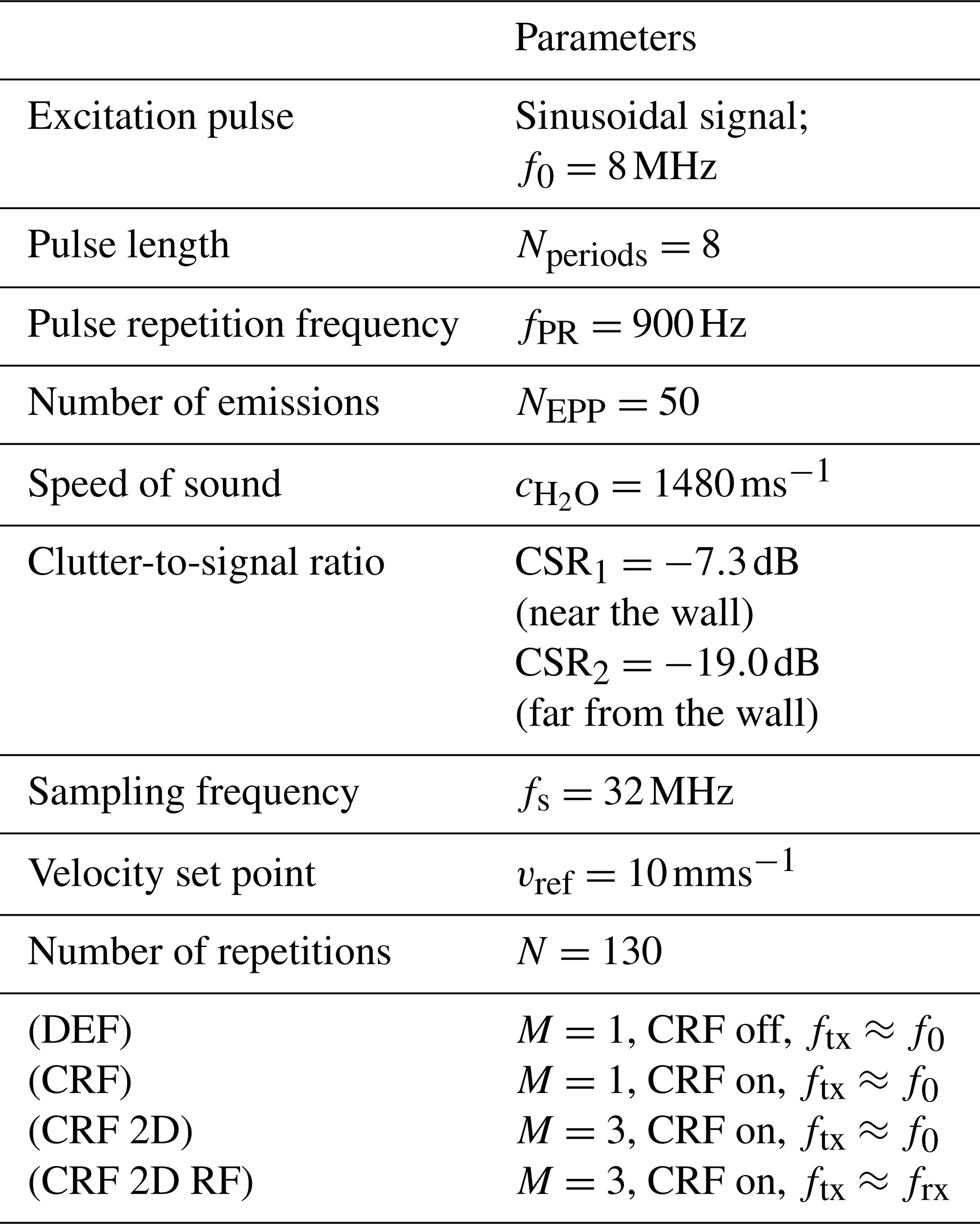
A total of 130 measurement cycles were conducted, consisting of a constant translation away from the front wall of the tank with a velocity set-point and the respective backward motion. Of the continuously obtained UADV measurements, only those that originate from two defined positions near to and far from the wall during the movement away from the ultrasound transducer (Richter Sensor and Transducer Technology, Germany) are selected in the postprocessing. The clutter-to-signal ratio (CSR) is and , respectively. To ensure a common time base for vibrometer and UADV measurements, the trigger signal of the UADV is acquired simultaneously with the velocity and position signals. To test the performance under different SNR conditions, white Gaussian noise was added to the raw digitized signals to achieve . Four algorithmic variants were compared as follows:
-
(DEF) – the 1D Kasai velocity estimator without clutter filtering, as described in Sect. 3.4
-
(CRF) – the 1D Kasai velocity estimator with a clutter filtering according to Sect. 3.3
-
(CRF 2D) – the 2D velocity estimator as described in Sect. 3.5 with clutter filtering but without an estimation of ftx
-
(CRF 2D RF) – the 2D velocity estimator as with clutter filtering including the estimation of ftx.
The parameterization of the experiment and of the algorithms is listed in Table 2.
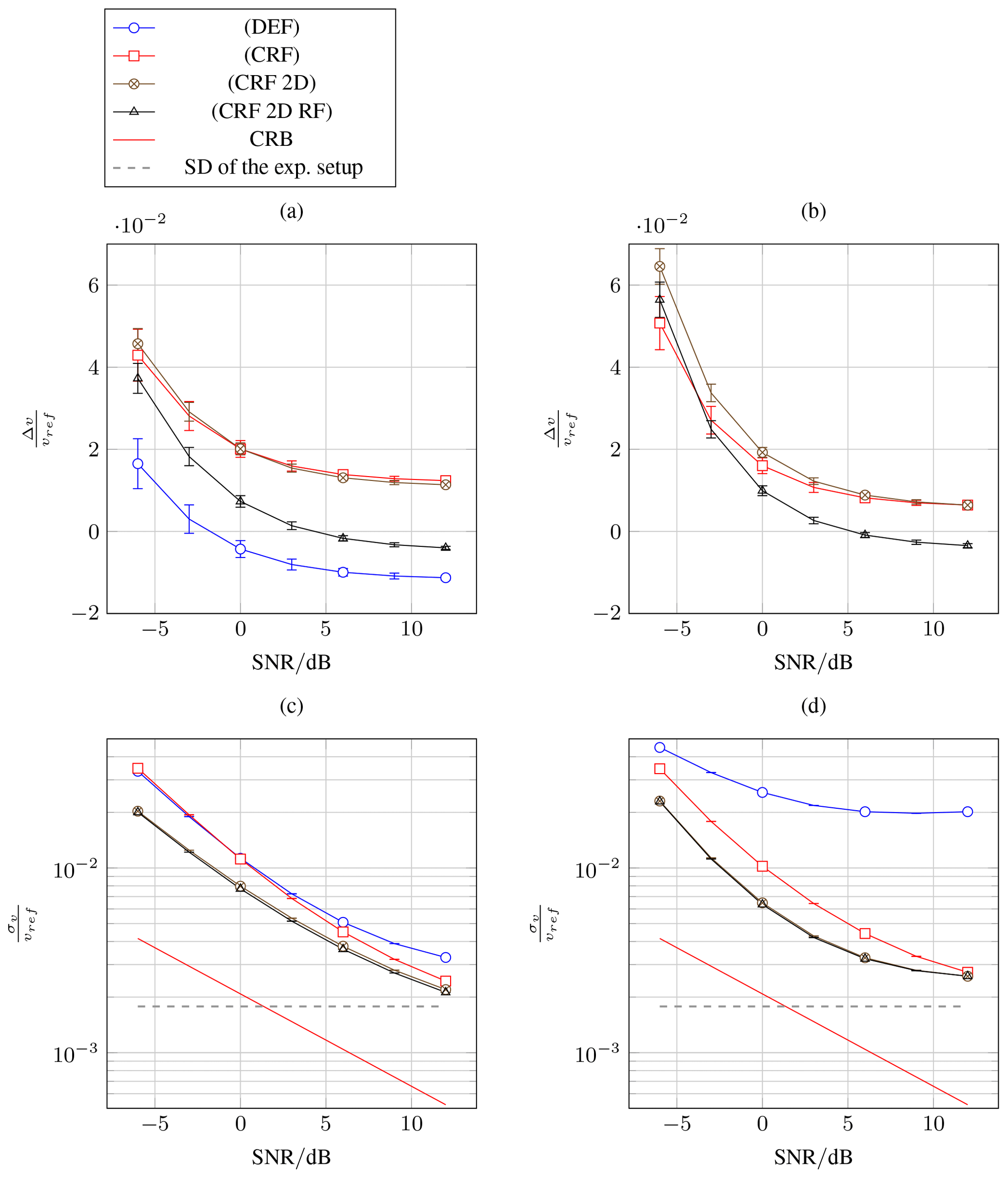
Figure 4Relative systematic deviation (a, b) and relative standard deviation (c, d) of the velocity versus SNR for reference measurements far from the wall (a, c) and near to the wall (b, d); the relative systematic deviation of (DEF) (b) is outside of the axis, with ; the error bars denote the 95 % confidence interval from 130 measurement cycles.

Figure 5Example of a flow image of magnetically stirred GaInSn in the central horizontal plane of a cubic vessel. Panel (a) depicts the experimental setup, (b) the mean flow velocity along the d axis, and (c) the standard deviation.
Table 3Measurement uncertainty budget for typical MHD experiments in liquid GaInSn.
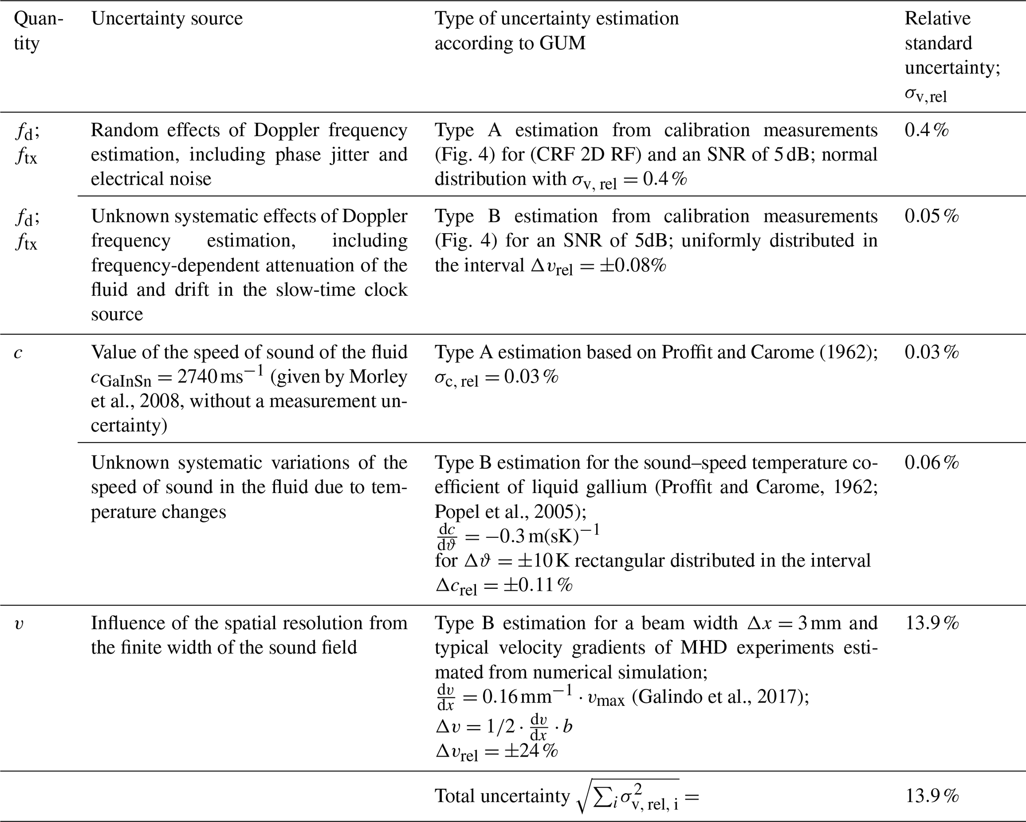
Figure 4 shows the relative systematic deviation from the reference velocity and the relative velocity standard deviation of the tested algorithms. For the low-CSR case (far from the wall) at SNR=12 dB, it can be seen that a slight negative bias of (DEF) is turned into a positive bias through clutter filtering (CRF) and (CRF 2D). This is compensated by the frequency estimation of (CRF 2D RF), which shows the lowest deviations of all variants for SNR≥3 dB. For the high-CSR case (near to the wall), the variant (DEF) without clutter filter has a relative deviation of . Through clutter filtering this strong negative bias is turned into a positive bias, which increases with lower SNR for (CRF) and (CRF 2D). The RF estimation of (CRF 2D RF) gives the lowest systematic bias for SNR≥0 dB. The relative standard deviations of all variants of the Kasai's algorithm do not reach the CRB for the given signal model, which is consistent with the findings of Chan et al. (2012). The lowest standard deviations are consistently provided by the variants (CRF 2D) and (CRF 2D RF), which come as close as a factor of 3 to the CRB by using more samples per gate than (DEF) and (CRF). For the given experimental data, the algorithm variant (CRF 2D RF) provides a suitable trade-off between systematic and standard deviation and computational complexity.
A measurement uncertainty budget according to the GUM (JCGM, 2008) is used to assess the contributions of measurement uncertainty for the UADV system. Based on Eq. (1), the measurand v is derived from the quantities fd, c and frx. Furthermore, the direct influence of the spatial averaging over the flow within the ultrasound beam width is considered. In Table 3, the uncertainties contribution of these quantities are given for a typical MHD experiment.
For the uncertainties of fd and frx, the results of Sect. 5.2 are transferred from the reference experiments in water to typical measurement conditions in low-melting liquid metals. The maximum relative systematic deviation and standard deviation for both investigated CSR and a typical SNR of SNR=5 dB are used to calculate the equivalent uncertainty of the velocity. The influence of an uncertainty in the fluid's speed of sound, c, is estimated by the uncertainty of the measurement of this quantity, in the literature and the temperature dependence, assuming a temperature gradient of . The uncertainty arising from spatial averaging through the ultrasound beam characteristics is calculated by assuming a lateral averaging of Δx=3 mm and velocity gradients of numerical simulations of typical MHD experiments (Galindo et al., 2017).
It can be seen that the biggest contribution to the velocity uncertainty of the UADV measurement system for typical MHD settings with stems from the spatial averaging over lateral resolution given by the ultrasound beam width of the unfocused transducers. This provides the most promising starting point for further improvements regarding the measurement uncertainty of the UADV system. Furthermore, it justifies the approximations taken for computationally efficiently implementing the signal processing, even though lower uncertainty algorithms exist that approach the CRB (Chan et al., 2012) because signal processing is not the limiting factor in the measurement uncertainty budget.
To demonstrate the capabilities of the ultrasound array Doppler velocimeter (UADV) with the proposed signal processing, it is applied to a simple MHD experiment. A cubic vessel with the dimensions of is filled with GaInSn and a 25-element linear transducer array (Richter Sensor and Transducer Technology, Germany) is attached to insonify the central horizontal plane (cf. Fig. 5a). With the application of a horizontally counterclockwise rotating magnet field, a counterclockwise central vortex forms. The UADV measures the velocity component along the axis of the transducers (d axis) with the parameterization given in Table 2 and with fPR=200 Hz. The resulting planar flow image, using signal-processing variant (CRF 2D RF), is shown in Fig. 5b and c.
Experimental research in the field of MHD can benefit from online, noninvasive flow imaging for investigating fundamental phenomena, such as flow instabilities and optimizing industrial processes. We describe an online-capable signal processing for pulsed-wave Doppler velocimetry that is tailored to the specific requirements of lab-scale model experiments. It is based on a 2D autocorrelator, which allows for a reduction of systematic and stochastic errors through explicitly estimating the RF and utilizing multiple samples per gate. We optimized the signal processing for low computational complexity and implemented substantial parts on an FPGA. A typical reduction of the data bandwidth of 6.5:1 enables continuous data streaming to PC hardware.
We evaluated the performance of the implemented signal processing in a water test rig with a single scattering object and a reference velocity obtained through a laser vibrometer. Two different clutter signal levels emulate a measurement close to and far from a wall. A velocity standard deviation of was found, which is about 3 times the fundamental limit of the uncertainty, the CRB, for velocity estimation. The systematic deviation is .
We investigated the measurement uncertainty budget for flow velocity measurements in a typical MHD experimental setup for the low-melting alloy GaInSn. The total measurement uncertainty of almost solely stems from the effect of spatial averaging over the lateral resolution for flows with high-velocity gradients. This justifies the approximations taken for lowering the computational complexity of the signal processing.
A measurement uncertainty budget of a typical MHD experiment at laboratory scale suggests improvements towards a better lateral resolution. In the context of flow imaging, this can be provided by the focusing and steering of the ultrasound beam using the phased-array principle.
The presented signal processing enables online, multiplane flow visualization with the UADV research platform. A long measurement duration (>1 h), combined with a high frame rate (>10 Hz), allows one to investigate complex, instationary flows such as instability phenomena in cubes.
Research data are available upon request from the authors.
RN implemented the signal processing, designed and conducted the numerical and experimental investigations. LB and JC supervised the research. All authors discussed and proofread the manuscript.
The authors declare that they have no conflict of interest.
The authors would like to thank the Deutsche Forschungsgemeinschaft (DFG) for their financial support (grant no. DFG BU 2241-2), Hannes Beyer for the FPGA-based implementation, Dirk Räbiger (Helmholtz-Zentrum Dresden-Rossendorf) for providing the GaInSn experimental setup, and Andreas Fischer (Bremen Institute for Metrology, Automation and Quality Science) for discussing the results.
This research has been supported by the Deutsche Forschungsgemeinschaft (grant no. DFG BU 2241-2).
This open-access publication was funded
by the Technische Universität Dresden (TUD).
This paper was edited by Marco Jose da Silva and reviewed by two anonymous referees.
Alam, S. and Parker, K. J.: Implementation issues in ultrasonic flow imaging, Ultrasound Med. Biol., 29, 517–528, https://doi.org/10.1016/S0301-5629(02)00704-4, 2003. a, b
Baker, D.: Pulsed Ultrasonic Doppler Blood-Flow Sensing, Sonics and Ultrasonics, IEEE T. Son. Ultrason., 17, 170–184, https://doi.org/10.1109/T-SU.1970.29558, 1970. a, b
Bjaerum, S., Torp, H., and Kristoffersen, K.: Clutter filter design for ultrasound color flow imaging, IEEE T. Ultrason. Ferr., 49, 204–216, 2002. a
Büttner, L., Nauber, R., Burger, M., Räbiger, D., Franke, S., Eckert, S., and Czarske, J.: Dual-plane ultrasound flow measurements in liquid metals, Meas. Sci. Technol., 24, 055302, https://doi.org/10.1088/0957-0233/24/5/055302, 2013. a
Chan, A., Lam, E., and Srinivasan, V.: Optimal doppler frequency estimators for ultrasound and optical coherence tomography, in: Biomedical Circuits and Systems Conference (BioCAS), IEEE, November 2012, Hsinchu, Taiwan, 264–267, https://doi.org/10.1109/BioCAS.2012.6418446, 2012. a, b, c
Cramér, H.: Mathematical Methods of Statistics, Princeton Press, Princeton, NJ, 367–369, 1946. a
Demirli, R. and Saniie, J.: Model-based estimation of ultrasonic echoes. Part I: Analysis and algorithms, IEEE T. Ultrason. Ferr., 48, 787–802, https://doi.org/10.1109/58.920713, 2001. a
Eckert, S., Cramer, A., and Gerbeth, G.: Velocity Measurement Techniques for Liquid Metal Flows, in: Magnetohydrodynamics, Fluid Mec. A., 80, 275–294, Springer Netherlands, https://doi.org/10.1007/978-1-4020-4833-3_17, 2007a. a
Eckert, S., Gerbeth, G., Räbiger, D., Willers, B., and Zhang, C.: Experimental modeling using low melting point metallic melts: Relevance for metallurgical engineering, Steel Res. Int., 78, 419–425, 2007b. a
Fischer, A., Pfister, T., and Czarske, J.: Derivation and comparison of fundamental uncertainty limits for laser-two-focus velocimetry, laser Doppler anemometry and Doppler global velocimetry, Measurement, 43, 1556–1574, https://doi.org/10.1016/j.measurement.2010.09.009, 2010. a, b
Furuichi, N.: Fundamental uncertainty analysis of flowrate measurement using the ultrasonic Doppler velocity profile method, Flow Meas. Instrum., 33, 202–211, https://doi.org/10.1016/j.flowmeasinst.2013.07.004, 2013. a
Galindo, V., Nauber, R., Räbiger, D., Franke, S., Beyer, H., Büttner, L., Czarske, J., and Eckert, S.: Instabilities and spin-up behaviour of a rotating magnetic field driven flow in a rectangular cavity, Phys. Fluids, 29, 114104, https://doi.org/10.1063/1.4993777, 2017. a, b, c
Gardin, P., Galpin, J.-M., Regnier, M.-C., and Radot, J.-P.: Liquid steel flow control inside continuous casting mold using a static magnetic field, IEEE T. Magn., 31, 2088–2091, https://doi.org/10.1109/20.376456, 1995. a
JCGM: Guide to the expression of uncertainty in measurement, Tech. rep., Joint Committee for Guides in Metrology (JCGM), 2008. a, b
Jensen, A.: Estimation of blood velocities using ultrasound: a signal processing approach, Cambridge University Press, 1996. a, b, c, d, e
Kantz, H., Kurths, J., and Mayer-Kress, G.: Nonlinear Analysis of Physiological Data, Springer Berlin Heidelberg, 2012. a
Kasai, C., Namekawa, K., Koyano, A., and Omoto, R.: Real-Time Two-Dimensional Blood Flow Imaging Using an Autocorrelation Technique, IEEE T. Son. Ultrason., 32, 458–464, https://doi.org/10.1109/T-SU.1985.31615, 1985. a, b, c, d, e
Kay, S. M.: Fundamentals of Statistical Signal Processing: Estimation Theory, Prentice-Hall, Inc., Upper Saddle River, NJ, USA, 1993. a
Lee, J., Cho, J., Yoo, Y. M., and kyong Song, T.: New clutter rejection method using time-domain averaging for ultrasound color Doppler imaging, in: Ultrasonics Symposium (IUS), September 2009, IEEE International, Rome, Italy, 1371–1374, https://doi.org/10.1109/ULTSYM.2009.5441639, 2009. a
Loupas, T., Peterson, R., and Gill, R.: Experimental evaluation of velocity and power estimation for ultrasound blood flow imaging, by means of a two-dimensional autocorrelation approach, IEEE T. Ultrason. Ferr., 42, 689–699, https://doi.org/10.1109/58.393111, 1995a. a
Loupas, T., Powers, J., and Gill, R.: An axial velocity estimator for ultrasound blood flow imaging, based on a full evaluation of the Doppler equation by means of a two-dimensional autocorrelation approach, IEEE T. Ultrason. Ferr., 42, 672–688, https://doi.org/10.1109/58.393110, 1995b. a, b
Lovstakken, L., Bjaernm, S., and Torp, H.: Optimal velocity estimation in ultrasound color flow imaging in presence of clutter, IEEE T. Ultrason. Ferr., 54, 539–549, https://doi.org/10.1109/TUFFC.2007.277, 2007. a
Morley, N. B., Burris, J., Cadwallader, L. C., and Nornberg, M. D.: GaInSn usage in the research laboratory, Rev. Sci. Instrum., 79, 056107, https://doi.org/10.1063/1.2930813, 2008. a
Müller, G. and Friedrich, J.: Optimization and modelling of photovoltaic silicon crystallization processes, in: AIP Conference Proceedings, Fourteenth International Summer School on Crystal Growth, vol. 1270, p. 255281, https://doi.org/10.1063/1.3476230, 2010. a
Nauber, R., Burger, M., Büttner, L., Franke, S., Räbiger, D., Eckert, S., and Czarske, J.: Novel ultrasound array measurement system for flow mapping of complex liquid metal flows, The European Physical Journal Special Topics, 220, 43–52, https://doi.org/10.1140/epjst/e2013-01795-1, 2013a. a
Nauber, R., Burger, M., Neumann, M., Büttner, L., Dadzis, K., Niemietz, K., Pätzold, O., and Czarske, J.: Dual-plane flow mapping in a liquid-metal model experiment with a square melt in a traveling magnetic field, Exp. Fluids, 54, 1–11, https://doi.org/10.1007/s00348-013-1502-x, 2013b. a
Nauber, R., Thieme, N., Radner, H., Beyer, H., Büttner, L., Dadzis, K., Pätzold, O., and Czarske, J.: Ultrasound flow mapping of complex liquid metal flows with spatial self-calibration, Flow Meas. Instrum., 48, 59–63, https://doi.org/10.1016/j.flowmeasinst.2015.12.005, 2016. a, b
Popel, P., Sidorov, V., Yagodin, D., Sivkov, G., and Mozgovoj, A.: Density and ultrasound velocity of some pure metals in liquid state, in: 7th European Conference on Thermophysical Properties, 2005. a
Proffit, R. and Carome, E.: Measurements of the velocity and absorption of ultrasound in liquid gallium, Tech. rep., DTIC Document, John Carroll University, Cleveland, Ohio, 1962. a, b
Radhakrishna Rao, C.: Information and accuracy attainable in the estimation of statistical parameters, Bull. Calcutta Math. S., 37, 81–91, 1945. a
Shung, K.: Diagnostic Ultrasound: Imaging and Blood Flow Measurements, Second Edition, CRC Press, 2015. a
Takeda, Y.: Velocity profile measurement by ultrasound Doppler shift method, Int. J. Heat Fluid Fl., 7, 313–318, https://doi.org/10.1016/0142-727X(86)90011-1, 1986. a
Thieme, N., Bönisch, P., Meier, D., Nauber, R., Büttner, L., Dadzis, K., Pätzold, O., Sylla, L., and Czarske, J.: Ultrasound Flow Mapping for the Investigation of Crystal Growth, IEEE T. Ultrason. Ferr., 64, 725–735, https://doi.org/10.1109/TUFFC.2017.2654124, 2017. a, b
Thomas, L. and Hall, A.: An improved wall filter for flow imaging of low velocity flow, in: 1994 Proceedings of IEEE Ultrasonics Symposium, Cannes, France, 31 October–3 November 1994, 3, 1701–1704, https://doi.org/10.1109/ULTSYM.1994.401918, 1994. a
Timmel, K., Eckert, S., and Gerbeth, G.: Experimental Investigation of the Flow in a Continuous-Casting Mold under the Influence of a Transverse, Direct Current Magnetic Field, Metall. Mater. Trans. A, 42, 68–80, https://doi.org/10.1007/s11663-010-9458-1, 2011. a, b
Torp, H.: Clutter rejection filters in color flow imaging: A theoretical approach, IEEE T. Ultrason. Ferr., 44, 417–424, 1997. a
Torp, H., Lai, X., and Kristoffersen, K.: Comparison between cross-correlation and auto-correlation technique in color flow imaging, in: 1993 Proceedings IEEE Ultrasonics Symposium, Baltimore, USA, 31 October–3 November 1993, 2, 1039–1042, https://doi.org/10.1109/ULTSYM.1993.339630, 1993. a
Turin, G.: An introduction to matched filters, IRE T. Inform. Theor., 6, 311–329, https://doi.org/10.1109/TIT.1960.1057571, 1960. a
Yasuda, H., Toh, T., Iwai, K., and Morita, K.: Recent Progress of EPM in Steelmaking, Casting, and Solidification Processing, ISIJ International, 47, 619–626, https://doi.org/10.2355/isijinternational.47.619, 2007. a
- Abstract
- Introduction
- Pulsed-wave ultrasound Doppler velocimetry
- Signal processing for velocity estimation
- Online-capable, FPGA-based signal-processing implementation
- Performance evaluation of narrow-band signal-processing algorithms
- Measurement uncertainty budget of the UADV in liquid metal
- Example of liquid metal flow imaging
- Conclusions
- Data availability
- Author contributions
- Competing interests
- Acknowledgements
- Financial support
- Review statement
- References